Low $T/|W|$ dynamical instability in differentially rotating stars: Diagnosis with canonical angular momentum

Abstract

We study the nature of non-axisymmetric dynamical instabilities in differentially rotating stars with both linear eigenmode analysis and hydrodynamic simulations in Newtonian gravity. We especially investigate the following three types of instability; the one-armed spiral instability, the low $T/|W|$ bar instability, and the high $T/|W|$ bar instability, where $T$ is the rotational kinetic energy and $W$ is the gravitational potential energy. The nature of the dynamical instabilities is clarified by using a canonical angular momentum as a diagnostic. We find that the one-armed spiral and the low $T/|W|$ bar instabilities occur around the corotation radius, and they grow through the inflow of canonical angular momentum around the corotation radius. The result is a clear contrast to that of a classical dynamical bar instability in high $T/|W|$. We also discuss the feature of gravitational waves generated from these three types of instability.

1 Introduction

Stars in nature are usually rotating and may be subject to non-axisymmetric rotational instabilities. An analytically exact treatment of these instabilities in linearized theory exists only for incompressible equilibrium fluids in Newtonian gravity (e.g., Chandrasekhar, 1969; Tassoul, 1978; Shapiro & Teukolsky, 1983). For these configurations, global rotational instabilities may arise from non-radial toroidal modes $e^{im\varphi}$ (where $m=\pm 1,\pm 2,\dots$ and $\varphi$ is the azimuthal angle).

For sufficiently rapid rotation, the $m=2$ bar mode becomes either secularly or dynamically unstable. The onset of instability can typically be marked by a critical value of the dimensionless parameter $\beta\equiv T/|W|$, where $T$ is the rotational kinetic energy and $W$ the gravitational potential energy. Uniformly rotating, incompressible stars in Newtonian theory are secularly unstable to bar-mode formation when $\beta\ga\beta_{\rm sec}\simeq 0.14$. This instability can grow only in the presence of some dissipative mechanism, like viscosity or gravitational radiation, and the associated growth time-scale is the dissipative time-scale, which is usually much longer than the dynamical time-scale of the system. By contrast, a dynamical instability to bar formation sets in when $\beta\ga\beta_{\rm dyn}\simeq 0.27$. This instability is present independent of any dissipative mechanism, and the growth time is the hydrodynamic time-scale.

In addition to the classical dynamical instability mentioned above, there have been several studies indicating that a dynamical instability of the rotating stars occurs at low $T/|W|$, which is far below the classical criterion of dynamical instability in Newtonian gravity. Tohline & Hachisu (1990) find in the self-gravitating ring and tori that an $m=2$ dynamical instability occurs around $T/|W|\sim 0.16$ in the lowest case in the centrally condensed configurations. For rotating stellar models, Shibata, Karino & Eriguchi (2002, 2003) find that $m=2$ dynamical instability occurs around $T/|W|\sim O(10^{-2})$ for a high degree ($\Omega_{\rm c}/\Omega_{\rm s}\approx 10$) of differential rotation. Note that $\Omega_{\rm c}$ and $\Omega_{\rm s}$ are the angular velocity at the centre and at the equatorial surface, respectively. Centrella et al. (2001) found dynamical $m=1$ instability around $T/|W|\sim 0.09$ in the $N=3.33$ polytropic ‘toroidal’ star with a high degree ($\Omega_{\rm c}/\Omega_{\rm s}=26$) of differential rotation, and Saijo, Baumgarte & Shapiro (2003) extended the results of dynamical $m=1$ instability to the cases with polytropic index $N\ga 2.5$ and $\Omega_{\rm c}/\Omega_{\rm s}\ga 10$.

Computation of the onset of the dynamical instability, as well as the subsequent evolution of an unstable star, performed in a fully nonlinear hydrodynamic simulation in Newtonian gravity, (e.g. Tohline, Durisen & McCollough, 1985; Durisen et al., 1986; Williams & Tohline, 1988; Houser, Centrella & Smith, 1994; Smith, Houser & Centrella, 1995; Houser & Centrella, 1996; Pickett, Durisen & Davis, 1996; Toman et al., 1998; New, Centrella & Tohline, 2000) have shown that $\beta_{\rm dyn}$ depends only very weakly on the stiffness of the equation of state. Once a bar has developed, the formation of a two-arm spiral plays an important role in redistributing the angular momentum and forming a core-halo structure. $\beta_{\rm dyn}$ are smaller for stars with high degree of differential rotation (Tohline & Hachisu, 1990; Pickett et al., 1996; Shibata et al., 2002, 2003). Simulations in relativistic gravitation (Shibata, Baumgarte & Shapiro, 2000; Saijo et al., 2001) have shown that $\beta_{\rm dyn}$ decreases with the compaction of the star, indicating that relativistic gravitation enhances the bar mode instability.

Recently, several studies have been focused on the collapse of the rotating stars leading to non-axisymmetric dynamical instabilities in three-dimensional hydrodynamics. Duez, Shapiro & Yo (2004) investigated the collapse of a differentially rotating $N=1$ polytropic star in full general relativity by depleting the pressure and found that the collapsing star forms a torus which fragments into nonaxisymmetric clumps. Shibata & Sekiguchi (2005) investigated rotational core collapse in full general relativity and found that a burst type of gravitational waves was emitted. In addition, they argued that a very limited window for the rotating star satisfies to exceed the threshold of dynamical instability in the core collapse. Saijo (2005) studied the spheroidal and toroidal configuration of the collapsing star in conformally flat gravity, and found that toroidal configuration has a potential source of gravitational waves due to the enhancement of the non-axisymmetric dynamical instability. Zink et al. (2005) presented a fragmentation of an $N=3$ toroidal polytropic star to both one-armed spiral and a binary system in full general relativity, depending on the type of initial density perturbation. There the authors confirm that the instabilities found in Newtonian gravity also appear in general relativistic stars of astrophysical relevance. Ott et al. (2005) performed gravitational collapse of unstable iron cores at the centre of evolved massive stars in Newtonian gravity. Their simulations contained the evolutions from implosion of iron core (the computations done in two-dimensional code) up to the post bounce phase, in which they found growth of unstable $m=1$, $2$ oscillations.

One of the remarkable features of these low $T/|W|$ instabilities is an appearance of the corotation modes. As it is pointed out by Watts, Andersson & Jones (2005) the low $T/|W|$ unstable oscillation of bar-typed one found by Shibata et al. (2002, 2003) has a corotation point. Here, corotation means the pattern speed of oscillation in the azimuthal direction coincides with a local rotational angular velocity of the star. It is well-known in the context of stellar or gaseous disk system that the corotation of oscillation may lead to instabilities. For instance, there have been several density wave models proposed to explain spiral pattern in galaxies, in which wave amplification at the corotation radius of spiral pattern is a key issue (Shu, 1992). Another example of importance of corotation is found in the theory of thick disk (torus) around black holes. Initiated by a discovery of a dynamical instability of geometrically thick disk by Papaloizou & Pringle (1984, 1985, 1987), several authors have studied these instabilities (Blaes, 1985a, b; Drury, 1985; Blaes & Glatzel, 1986; Goldreich, Goodman & Narayan, 1986; Kojima, 1986, 1989; Glatzel, 1987a, b; Goodman & Narayan, 1988). Instabilities of these systems are thought not to be unique in their origin and in their characteristics. Some seem to be related to local shear of flow and to share a nature with Kelvin-Helmholtz instability. Others may be related to corotation of oscillation modes with averaged flow on which the oscillation is present. The mechanisms of instabilities by corotation, however, seem not unique. As is reminiscent to ‘Landau amplification’ of plasma wave (Stix, 1992), a resonant interaction of corotating wave with the background flow (in the case of Landau amplification, background flow is that of charged particles) may amplify the wave, by direct pumping of energy from background flow to the oscillation. The other may be an overreflection of waves at the corotation which may be seen in waves propagating towards shear layer (Acheson, 1976).

The main purpose of this paper, in contrast to the preceding studies of this issue, is to investigate the nature of low $T/|W|$ dynamical instabilities, especially to study the qualitative difference of them from the classical bar instability. As is mentioned above, recent studies have shown that dynamical instabilities are possible for different region of the parameter space of rotating stars. Observing the existence of dynamical instabilities whose critical $T/|W|$ value are well below the classical criterion of bar instability, it is natural to raise a question on whether these two types, ‘high $T/|W|$’ and ‘low $T/|W|$’, of dynamical instability are categorized in the same type of dynamical instability or not.

Our study is done with both eigenmode analysis and hydrodynamical analysis. A non-linear hydrodynamical simulation is indispensable for investigation of evolutionary process and final outcome of instability, such as bar formation and spiral structure formation. The nature of instability as a source of gravitational wave, which interests us most, is only accessible through non-linear hydrodynamical computations. On the other hand, a linear eigenmode analysis is in general easier to approach the dynamical instability of a given equilibrium and it may be helpful to have physical insight on the mechanism and the origin of the instability. Therefore, a linear eigenmode analysis and a non-linear simulation are complementary to each other and they both help us to understand the nature of dynamical instability.

As a simplified system mimicking the physical nature of the differentially rotating fluid, we choose to study self-gravitating cylinder models. They have been used to study general dynamical nature of such gaseous masses as stars, accretion disks and of stellar system as galaxies. Although there is no infinite-length cylinder in the real world, it is expected to share some qualitative similarities with realistic astrophysical objects (Ostriker, 1965; Robe, 1979; Balbinski, 1985; Ishibashi & Ando, 1985, 1986; Blaes & Glatzel, 1986; Glatzel, 1987a, b; Luyten, 1988, 1989, 1990; Cook, Shapiro & Stephans, 2003). Especially it has served as a useful model to investigate secular and dynamical instabilities of rotating masses. These works took advantage of a simple configuration of a cylinder compared with a spheroid.

This paper is organized as follows. In Sections 2 and 3 we present our hydrodynamical and eigenmode analysis results of dynamical one-armed spiral and dynamical bar instability. We present our diagnosis of dynamical $m=1$ and $m=2$ instabilities by using a canonical angular momentum in Section 4, and summarize our findings in Section 5. Throughout this paper we use gravitational units with $G=1$. Latin indices run over spatial coordinates.

2 Hydrodynamic simulations in Differentially Rotating Stars

Here, we briefly describe the basic equation of the perfect fluid hydrodynamics in Newtonian gravity. We follow Saijo et al. (2003) to perform our $3$ dimensional Newtonian hydrodynamics assuming an adiabatic $\Gamma$-law equation of state

$$P=(\Gamma-1)\rho\varepsilon,$$ (2.1)

where $P$ is the pressure, $\Gamma$ the adiabatic index, $\rho$ the mass density and $\varepsilon$ the specific internal energy density. For perfect fluids, the Newtonian equations of hydrodynamics then consist of the continuity equation

$$\frac{\partial\rho}{\partial t}+\frac{\partial(\rho v^{i})}{\partial x^{i}}=0,$$ (2.2)

the energy equation

$$\frac{\partial e}{\partial t}+\frac{\partial(ev^{j})}{\partial x^{j}}=-\frac{1}{\Gamma}e^{-(\Gamma-1)}P_{\rm vis}\frac{\partial v^{i}}{\partial x^{i}},$$ (2.3)

and the Euler equation

$$\frac{\partial(\rho v_{i})}{\partial t}+\frac{\partial(\rho v_{i}v^{j})}{\partial x^{j}}=-\frac{\partial(P+P_{\rm vis})}{\partial x^{i}}-\rho\frac{\partial\Phi}{\partial x^{i}}.$$ (2.4)

Here $v^{i}$ is the fluid velocity, $\Phi$ is the gravitational potential

$$\triangle\Phi=4\pi\rho,$$ (2.5)

and $e$ is defined according to

$$e=(\rho\varepsilon)^{1/\Gamma}.$$ (2.6)

We use the same type of artificial viscosity pressure $P_{\rm vis}$ in Saijo et al. (2003). When evolving the above equations we limit the stepsize $\Delta t$ by an appropriately chosen dynamical time.

We construct differentially rotating equilibrium stars based on Hachisu (1986). We assume a polytropic equation of state only to construct an equilibrium star as

$$P=\kappa\rho^{1+1/N},$$ (2.7)

where $\kappa$ is a constant, $N$ is the polytropic index. We also assume the ‘$j$-constant’ rotation law, which has an exact meaning in the limit of $d\rightarrow 0$, of the rotating stars

$$\Omega=\frac{j_{0}}{d^{2}+\varpi^{2}},$$ (2.8)

where $\Omega$ is the angular velocity, $j_{0}$ is a constant parameter with units of specific angular momentum, and $\varpi$ is the cylindrical radius. The parameter $d$ determines the length scale over which $\Omega$ changes; uniform rotation is achieved in the limit $d\rightarrow\infty$, with keeping the ratio $j_{0}/d^{2}$ finite. We choose the same data sets as Saijo et al. (2003) for investigating low $T/|W|$ dynamical instabilities in differentially rotating stars (models I and II in Table 1 corresponds to Tables II and I of Saijo et al. (2003), respectively). We also construct an equilibrium star with weak differential rotation in high $T/|W|$, which excites the standard dynamical bar instability, (e.g., Chandrasekhar, 1969). The characteristic parameters are summarized in Table 1.

To enhance any $m=1$ or $m=2$ instability, we disturb the initial equilibrium mass density $\rho_{\rm eq}$ by a non-axisymmetric perturbation according to

$$\rho=\rho_{\rm eq}\left(1+\delta^{(1)}\frac{x+y}{R_{\rm eq}}+\delta^{(2)}\frac{x^{2}-y^{2}}{R_{\rm eq}^{2}}\right),$$ (2.9)

where $R_{\rm eq}$ is the equatorial radius, with $\delta^{(1)}=\delta^{(2)}\approx 1.7-2.8\times 10^{-3}$ in all our simulations. We also introduce ‘dipole’ $D$ and ‘quadrupole’ $Q$ diagnostics to monitor the development of $m=1$ and $m=2$ modes as

$$D = \left<e^{im\varphi}\right>_{m=1}=\frac{1}{M}\int\rho\frac{x+iy}{\varpi}dV,$$ (2.10)

$$Q = \left<e^{im\varphi}\right>_{m=2}=\frac{1}{M}\int\rho\frac{(x^{2}-y^{2})+i(2xy)}{\varpi^{2}}dV,$$

respectively.

We compute approximate gravitational waveforms by using the quadrupole formula. In the radiation zone, gravitational waves can be described by a transverse-traceless, perturbed metric $h_{ij}^{TT}$ with respect to flat spacetime. In the quadrupole formula, $h_{ij}^{TT}$ is found from (Misner, Thorne & Wheeler, 1973)

$$h_{ij}^{TT}=\frac{2}{r}\frac{d^{2}}{dt^{2}}I_{ij}^{TT},$$ (2.12)

where $r$ is the distance to the source, $I_{ij}$ the quadrupole moment of the mass distribution, and where $TT$ denotes the transverse-traceless projection. Choosing the direction of the wave propagation to be along the rotational axis ($z$-axis), the two polarization modes of gravitational waves can be determined from

$$h_{+}\equiv\frac{1}{2}(h_{xx}^{TT}-h_{yy}^{TT}),\quad h_{\times}\equiv h_{xy}^{TT}.$$ (2.13)

For observers along the rotation axis, we thus have

$$\frac{rh_{+}}{M} = \frac{1}{2M}\frac{d^{2}}{dt^{2}}(I_{xx}^{TT}-I_{yy}^{TT}),$$ (2.14)

$$\frac{rh_{\times}}{M} = \frac{1}{M}\frac{d^{2}}{dt^{2}}I_{xy}^{TT}.$$ (2.15)

Table 1: Three differentially rotating equilibrium stars that trigger dynamical instability.

Model	$N^{a}$	${d/R_{\rm eq}}^{b}$	${R_{\rm p}/R_{\rm eq}}^{c}$	${\Omega_{\rm c}/\Omega_{\rm s}}^{d}$	${\rho_{\rm c}/\rho_{\rm max}}^{e}$	${R_{\rm maxd}/R_{\rm eq}}^{f}$	${T/|W|}^{g}$	Dominant unstable mode
I	$3.33$	$0.20$	$0.413$	$26.0$	$0.491$	$0.198$	$0.146$	$m=1$
II	$1.00$	$0.20$	$0.250$	$26.0$	$0.160$	$0.383$	$0.119$	$m=2$
III	$1.00$	$1.00$	$0.250$	$2.0$	$0.837$	$0.388$	$0.277$	$m=2$

${}^{a}N$: polytropic index. ${}^{b}R_{\rm eq}$: equatorial radius. ${}^{c}R_{\rm pl}$: polar radius. ${}^{d}\Omega_{\rm c}$: central angular velocity; $\Omega_{\rm s}$: equatorial surface angular velocity. ${}^{e}\rho_{\rm c}$: central mass density; $\rho_{\rm max}$: maximum mass density. ${}^{f}R_{\rm maxd}$: radius of maximum density. ${}^{g}T$: rotational kinetic energy; $W$: gravitational binding energy.

The time evolutions of the dipole diagnostic and the quadrupole diagnostic are plotted in Fig. 1. We determine that the system is stable to $m=1$ ($m=2$) mode when the dipole (quadrupole) diagnostic remains small throughout the evolution, while the system is unstable when the diagnostic grows exponentially at the early stage of the evolution. It is clearly seen in Fig. 1 that the star is more unstable to the one-armed spiral mode for model I, and more unstable to the bar mode for models II and III. In fact, both diagnostics grow for model I. The dipole diagnostic, however, grows larger than the quadrupole diagnostic, indicating that the $m=1$ mode is the dominant unstable mode.

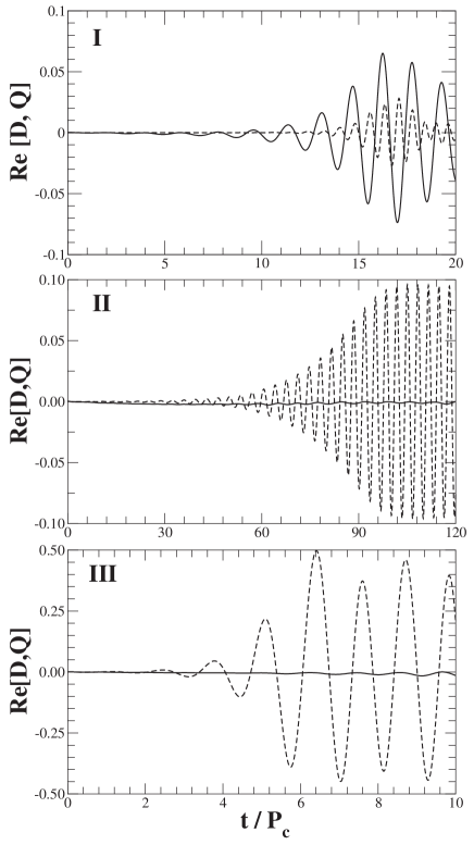
Figure 1: Diagnostics $D$ and $Q$ as a function of $t/P_{\rm c}$ for three differentially rotating stars (see Table 1). Solid and dotted lines denote the values of $D$ and $Q$, respectively. The Roman numeral in each panel corresponds to the model of the differentially rotating stars, respectively. Hereafter $P_{\rm c}$ represents the central rotation period.

The density contour of the differentially rotating stars are shown in Fig. 2 for the equatorial plane and in Fig. 3 for the meridional plane. It is clearly seen in Fig. 2 that one-armed spiral structure is formed at the intermediate stage of the evolution for model I, and that bar structure is formed for models II and III once the dynamical instability sets in.

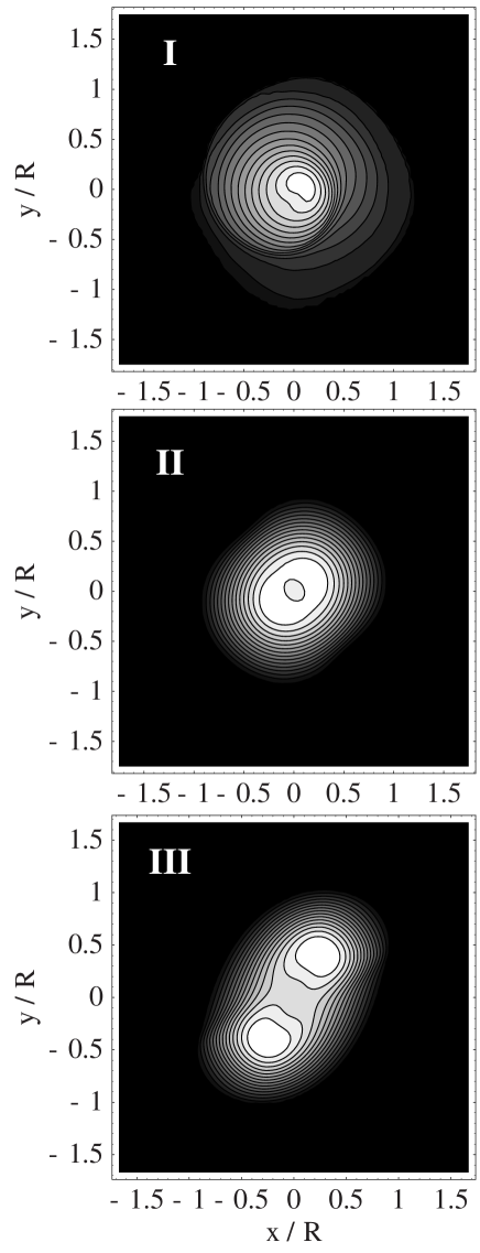
Figure 2: Density contours in the equatorial plane for three differentially rotating stars (see Table 1). Models I, II, and III are plotted at the parameter ($t/P_{\rm c}$, $\rho_{\rm max}/\rho_{\rm max}^{(0)}$) = ($16.2$, $3.63$), ($134$, $1.26$), and ($5.49$, $1.20$), where $\rho_{\rm max}$ is the maximum density, $\rho_{\rm max}^{(0)}$ is the maximum density at $t=0$, and $R$ is the equatorial radius at $t=0$. The contour lines denote densities $\rho/\rho_{\rm max}=10^{-(16-i)\times 0.287}(i=1,\cdots,15)$ for model I and $\rho/\rho_{\rm max}=6.67(16-i)\times 10^{-2}(i=1,\cdots,15)$ for models II and III, respectively.

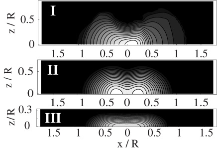
Figure 3: Density contours in the meridional plane for three differentially rotating stars (see Table 1). The parameters and the contour levels are the same as Fig. 2.

We show velocity fields in Fig. 4 in the equatorial plane and in Fig. 5 in the meridional plane during the evolution. Note that shocks occur during the formation of $m=1$ instability. We also find that the fluid motion of the $z$-direction does not play a dominant role in generating the dynamical instabilities.

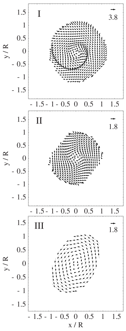
Figure 4: Velocity field ($v^{i}/|v_{\rm s}^{i~{}{\rm(0)}}|$) in the equatorial plane for three differentially rotating stars (see Table 1). The time for each snapshot is the same as in Fig. 2. Note that the velocity arrows are normalized as indicated in the upper right hand corner of each snapshot. $|v_{\rm s}^{i~{}{\rm(0)}}|$ denotes the surface absolute velocity at $t=0$.

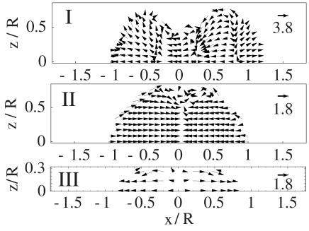
Figure 5: Velocity field ($v^{i}/|v_{\rm s}^{i~{}{\rm(0)}}|$) in the meridional plane for three differential rotating stars (see Table 1). The time for each snapshot is the same as in Fig. 2.

We also show gravitational waves generated from dynamical one-armed spiral and bar instabilities in Fig. 6. For $m=1$ modes, the gravitational radiation is emitted not by the primary mode itself, but by the $m=2$ secondary harmonic which is simultaneously excited, albeit at the lower amplitude. Unlike the case for bar-unstable stars, the gravitational wave signal does not persist for many periods, but instead damp fairly rapidly.

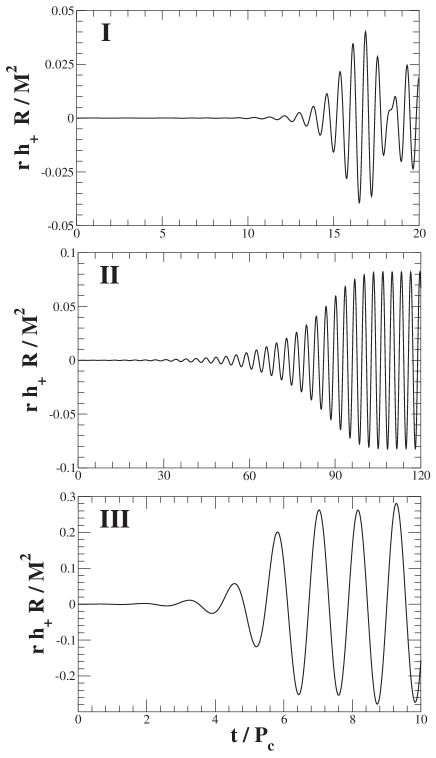
Figure 6: Gravitational waveform for three differentially rotating stars (see Table 1) as seen by a distant observer located on the rotational axis of the equilibrium star.

3 Stability analysis of a differentially rotating cylinder

3.1 Rotating selfgravitating cylinder model

Ostriker (1965) numerically computed physical characters of non-rotating infinite cylindrical masses. We here follow his treatment and introduce the normalization of variables.

A cylinder rotates around its axis with a given angular velocity profile, which is a function of a cylindrical radial coordinate $\varpi$. An equilibrium of the cylinder is determined by the balance between pressure gradient, centrifugal force and self-gravity of the cylinder. We also introduce an azimuthal angular coordinate $\varphi$, and a $z-$coordinate set along the axis of the cylinder.

For a fluid equation of state, we assume to have a polytropic relation

$$\rho=\rho_{\rm c}\bar{\theta}^{N},\quad p=p_{\rm c}\bar{\theta}^{N+1},$$ (3.1)

where $\rho_{c}$ and $p_{c}$ are the normalization factors for a mass density and a pressure, which we choose those values on the rotational axis of the cylinder, $N$ is a polytropic index. A variable with a bar denotes a normalized one. As shall be seen below, it is possible to construct a cylinder with a finite cylindrical radius by using large $N$. A non-rotating spheroid with $N\geq 5$ has an infinite radius, while a cylinder with $N=25$ still has a finite cylindrical radius. This qualitative difference from the well-known characteristics of spheroid simply results from the difference of geometry.

We normalize the cylindrical radial coordinate as $\varpi=\alpha\bar{\varpi}$, where $\alpha=\sqrt{(N+1)/4\pi G}$, and the rotational angular frequency as $\Omega=\bar{\Omega}\sqrt{4\pi G\rho_{c}}$. Following a similar procedure to obtain Lane-Emden equation of spherical polytropes, more specifically, with using $\varpi-$ component of the Euler equation and Poisson equation for a gravitational potential, we obtain Lane-Emden equation for a differentially rotating cylinder as

$$\frac{d^{2}\bar{\theta}}{d\bar{\varpi}^{2}}+\frac{1}{\bar{\varpi}}\frac{d\bar{\theta}}{d\bar{\varpi}}+\bar{\theta}^{N}=2\bar{\Omega}\frac{d}{d\bar{\varpi}}\left[\bar{\varpi}\bar{\Omega}\right].$$ (3.2)

The rotational profile of an angular velocity we study here is the same as the one used in the hydrodynamical simulations (equation 2.8),

$$\bar{\Omega}=\frac{B}{\bar{\varpi}^{2}+A},$$ (3.3)

where $A$ and $B$ are parameters. This is the same as equation (2.8), with $d=\sqrt{A}$ and $j_{0}=B$. For simplicity, we hereafter omit ‘bars’ from all the equations.

A frequently used dimensionless measure of rotation is $T/|W|$. The rotational kinetic energy $T$ is defined as

$$T=\frac{1}{2}\int\rho\varpi^{2}\Omega^{2}dV,$$ (3.4)

where integration is done for cylinder of unit length. As to gravitational energy, we follow the definition in Cook et al. (2003) as

$$W\equiv-\int\rho n^{i}\nabla_{i}\Phi dV=-\frac{m(\varpi)^{2}}{4\pi}.$$ (3.5)

Here, $\Phi$ is the gravitational potential and $n^{i}$ is a unit normal vector of $\varpi=$const. surface. The integration is performed for a unit length along the axis. $m(\varpi)$ is the mass contained inside the cylindrical radius per unit length.

For a large degree of differential rotation, the density maximum of the configuration becomes off-centred. An example of the profile of Lane-Emden function in such a case is plotted in Fig. 7.

Figure 7: Equilibrium profile of Lane-Emden function for a polytropic index $N=25$ and parameters of rotation $(A,B)=(0.43,1.6)$. Note that $T/|W|=0.452$. We find an $m=1$ unstable mode in corotation in this case.

3.2 Linear perturbation of a cylinder

3.2.1 Perturbation equations

To study linearized oscillations of selfgravitating cylinder, we simultaneously solve linearized version of (1) equation of continuity; (2) Euler equation; (3) Poisson equation for a gravitational potential. The adiabatic index of a perturbed fluid is assumed to coincide with that of background one, so that no $g$-mode appears in our computation. We also assume that there is no motion along the rotational axis of the cylinder, and therefore no dependence of the quantities on $z$-coordinate.

Assuming a simple harmonic dependence of Eulerian perturbation of variable $f$ as

$$\delta f(t,\varpi,\varphi)=\delta f_{1}(\varpi)\exp(-i\sigma t+im\varphi),$$ (3.6)

we can write down the perturbed equations as follows.
Equation of continuity:

$$\frac{du}{d\varpi}+\frac{Ns}{\theta}q+\left(\frac{N}{\theta}\frac{d\theta}{d\varpi}+\frac{1}{\varpi}\right)u-\frac{mv}{\varpi}=0.$$ (3.7)

$\varpi$-component of Euler equation:

$$su+2\Omega v=\frac{dq}{d\varpi}+\frac{dy}{d\varpi}.$$ (3.8)

$\varphi$-component of Euler equation:

$$s~{}v+\frac{\kappa^{2}}{2\Omega}u=\frac{m(q+y)}{\varpi},$$ (3.9)

where $\kappa:=\sqrt{2\Omega\left(2\Omega+\varpi d\Omega/d\varpi\right)}$ is the epicyclic frequency.
Poisson equation for a gravitational potential

$$\frac{d^{2}y}{d\varpi^{2}}+\frac{1}{\varpi}\frac{dy}{d\varpi}-\frac{m^{2}}{\varpi^{2}}y=N\theta^{N-1}q.$$ (3.10)

We have here defined Eulerian perturbation quantities as

$$u=i\cdot\delta v_{1}^{\varpi},\quad v=\delta v_{1}^{\varphi},\quad y=\delta\Phi_{1},\quad q=\delta\theta_{1}.$$ (3.11)

We also define the following quantity

$$s(\varpi)=\sigma-m\Omega(\varpi).$$ (3.12)

If $s=0$ for a certain cylindrical radius, the equations becomes singular there. We call it corotation singularity. In that case, a corotation radius $\varpi_{\rm crt}$ is defined as this singular point. Corotation radius corresponds to a cylindrical surface on which the pattern speed of the oscillation $\Re[\sigma/m]$ is equal to the local angular frequency of the background flow, $\Omega(\varpi_{\rm crt})$. Although $s=0$ is satisfied only for a purely real eigenfrequency, we here denote that a mode is in corotation when a cylindrical radius satisfies $\Re[\sigma]-m\Omega=0$ in the cylinder, even if we have a complex eigenfrequency $\sigma$. Thus a corotation radius is also defined for complex mode where the equation has no singularity.

Figure 8: Imaginary part of the eigenfrequency $\sigma$ for a dynamically unstable $m=1$ mode in a cylinder with $A=0.6$. Note that a polytropic index $N$ is $25$. The parameters of models marked as (a) to (d) are listed in Table 2.

To close the eigenvalue problem, we should impose boundary conditions. One of the two conditions at the surface $\varpi=\varpi_{\rm s}$ where equilibrium pressure becomes zero is the conventional free boundary condition. This means no stress is exerted on the cylindrical surface, which reduces to the condition:

$$sq+\frac{d\theta}{d\varpi}u=0.$$ (3.13)

The other is the condition on the perturbed gravitational potential. From equation (3.10), the perturbed potential outside the cylinder ($\theta=0$, $q=0$) is $y\sim\varpi^{\pm m}$. At the surface of the cylinder we impose the condition that the gravitational potential smoothly matches to the non-diverging solution at infinity. Therefore, the continuity condition of the potential requires

$$\frac{dy}{d\varpi}+\frac{m}{\varpi}y=0,$$ (3.14)

at the cylindrical surface. On the rotational axis of the cylinder, $\varpi=0$, we impose a regularity condition on the variables.

Our numerical method to solve this eigenvalue problem is straightforward: We use the conventional shooting method to find eigenmodes. The system of linearized equations are solved both from the rotational axis and from the surface of the cylinder, with the boundary conditions being taken into account. At the intermediate matching radius, we impose a condition that both solutions connect smoothly. This procedure picks up the physical solutions of the eigenvalue problem.

Figure 9: Eigenfunction of an unstable $m=1$ mode in $N=25$ cylinder. We normalize the cylindrical radius $\varpi$ with the surface radius $\varpi_{s}$. Real part of Lane-Emden function $q=\delta\theta$ are plotted. Note that the normalization of the eigenfunction is arbitrarily. The label (a) to (d) in the figure correspond to the model in Table 2.

As we are interested in a dynamical instability, we assume the eigenfrequency takes complex values as well as other perturbed variables. We focus to the case where $s(\varpi)=\sigma-\Omega(\varpi)$ is non-zero, which is true except for a real $\sigma$ at the corotation region, i.e., $\Omega(\varpi=\varpi_{\rm s})\leq\sigma\leq\Omega(\varpi=0)$. As a result, our present code can compute modes without corotation singularity. We also find convergence to ‘modes’ whose frequency is in the corotation region on the real axis of $\sigma$ plane. Although the ‘eigenfunction’ of it suggest that we are picking up one of the singular eigenmodes from continuous spectrum, we cannot prove it by our present code.

3.2.2 Characters of $m=1$ unstable eigenmode

First we note that we find unstable $m=1$ mode only for extremely soft equation of state. In general, we can construct a cylinder with a finite cylindrical radius (but an infinite length for $z$-direction) for an extremely large polytropic index $N$ than the case of a spheroid.

From the results of hydrodynamical simulations (Saijo et al., 2003), we find that an $m=1$ instability appears in a soft equation of state ($N\ga 2.5$). However in case of a cylinder, $N$ should satisfy $N\ga 20$ to find an $m=1$ instability. This is a drawback of the cylinder to be compared with a result of the spheroid, although the behaviour of the unstable mode is similar to the spheroid. We expect that a qualitative nature of these modes are similar even the polytropic indices are quite different.

For a fixed polytropic index, we have two parameters $A$ and $B$ to specify an equilibrium model. We construct a sequence fixing $A$ with changing $B$, which roughly corresponds to changing $T/|W|$ in a fixed degree of differential rotation. We summarize the characteristics of models studied in this paper in Table 2.

In Fig. 8 we plot an imaginary part of the eigenfrequency of $m=1$ mode as a function of $T/|W|$, fixing $A=0.6$ and $N=25$. The mode has a corotation radius inside the cylinder. The unstable mode appears only in a limited range of $T/|W|$. This behaviour of the imaginary part of the eigenfrequency is almost insensitive to the degree of differential rotation which is parametrized by $\sqrt{A}$.

Table 2: Parameters for equilibrium models and eigenfrequency of $m=1$ and $m=2$ modes. Models (a)-(d) correspond to those in Fig. 9.

Model	mode	$N$	$\Omega_{\rm c}/\Omega_{\rm s}$	$T/|W|$	${\sigma/\Omega_{c}}^{a}$	${\varpi_{\rm crt}/\varpi_{\rm s}}^{b}$
(a)	$m=1$	25	13.96	0.4543	$0.5126+0.01726i$	0.2709
(b)	$m=1$	25	11.34	0.4597	$0.5512+0.03153i$	0.2806
(c)	$m=1$	25	8.218	0.4675	$0.6281+0.03982i$	0.2864
(d)	$m=1$	25	6.067	0.4722	$0.6910+0.01716i$	0.2715
(b)-s1	$m=1$	25	11.34	0.4597	$-0.245~{}(\mbox{real})$	—
(b)-s2	$m=1$	25	11.34	0.4597	$1.15~{}(\mbox{real})$	—
(e)	$m=2$	1	13.00	0.170	$0.3269+0.01256i$	0.507

${}^{a}\sigma$: eigenfrequency of the mode. ${}^{b}\varpi_{\rm crt}$: corotation radius; $\varpi_{\rm s}$: surface radius.

Interestingly, this is reminiscent to the character of low-$T/|W|$ bar ($m=2$) instability which is recently found by Shibata et al. (2002, 2003) (see Fig. 3 in Shibata et al. (2003)). For a fixed degree of differential rotation, $T/|W|$ that permits unstable mode is limited in a finite range. This may suggest that $m=1$ instability and low-$T/|W|$ bar instability may have the same (or similar) generation mechanism.

We note that a real part of eigenfrequency is monotonically increasing function of $T/|W|$ and of the degree of differential rotation (see Table 2). The frequency is the order of unity for all cases here. For each equilibrium model with a sufficiently large degree of differential rotation and a limited range of $T/|W|$, we find unstable $m=1$ modes in the corotation. Note that we also have exponentially damping modes, whose eigenfrequency are the complex conjugate of the dynamically unstable modes. We also find discrete stable modes outside the corotation region, which have a purely real eigenfrequency. For equilibrium models where we found unstable $m=1$ corotating modes, we did not find any dynamically unstable $m=1$ mode outside the corotation.

We show the real part of the eigenfunction $q$ of an $m=1$ unstable mode in Fig. 9. In order to compare the $m=1$ eigenfunction of the linear analysis with that of the hydrodynamical simulation, we plot a perturbed mass density in a cylinder model (Fig. 10) and a perturbed $m=1$ unstable mass density in a differentially rotating star (Fig. 11). In order to compute the perturbed $m=1$ unstable mass density in a differentially rotating star, we follow

$$\delta\rho = \rho(t)-\rho_{\rm eq},$$ (3.15)

$$\delta\rho_{m=1} = \frac{1}{2\pi}\int\delta\rho~{}e^{-i\varphi}d\varphi.$$ (3.16)

We have a common feature that the $m=1$ unstable mass density has a single oscillation inside the star and in the cylinder. However the behavior is quite different: for a cylinder the oscillation is concentrated inside the corotation radius, while for the differentially rotating star the oscillation is spread out to the whole equatorial surface radius.

Figure 10: Perturbed mass density of an unstable $m=1$ mode for model (b) (see Table 2). As it is a solution of linear problem, the scaling is arbitrarily chosen.

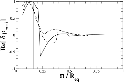
Figure 11: Amplitude of perturbed mass density of an unstable $m=1$ mode for model I (See Table 1). Note that the amplitude is normalized with its maximum. Solid, dashed, and dash-dotted lines represent $t=8.15P_{c}$, $9.32P_{c}$, and $10.48P_{c}$, respectively. Vertical line represents the corotation radius of the rotating star.

In order to focus on the comparison of the spiral structure of the $m=1$ unstable mode, we introduce a phase-constant curve of a perturbed radial velocity. In the linear analysis, complex velocity $\delta v^{\varpi}$ is written as (we omit the factor of time dependence $e^{-i\sigma t}$ since it is not relevant to a momentary spacial pattern)

$$\delta v^{\varpi}=U(\varpi)e^{iS(\varpi)+im\varphi},$$ (3.17)

where $U(\varpi)$ is a real amplitude and $S(\varpi)$ is a phase function. An equation defining phase-constant pattern is therefore,

$$S(\varpi)+m\varphi=\tan^{-1}\frac{\Im[\delta v^{\varpi}]}{\Re[\delta v^{\varpi}]}+m\varphi\equiv{\rm const.}$$ (3.18)

In a similar way, we also obtain a phase-constant pattern from the result of nonlinear hydrodynamical simulation. First we expand a perturbed radial velocity in the equatorial plane in terms of $\varphi$ as

$$\delta v^{\varpi}=\delta v^{\varpi}_{m}e^{im\varphi}=\|\delta v^{\varpi}_{m}\|~{}e^{i(m\varphi+S_{m})},$$ (3.19)

where

$$\delta v^{\varpi}_{m} = \frac{1}{2\pi}\int\delta v^{\varpi}~{}e^{-im\varphi}d\varphi,$$ (3.20)

$$\|v^{\varpi}_{m}\| = \sqrt{(\Re[\delta v^{\varpi}_{m}])^{2}+(\Im[\delta v^{\varpi}_{m}])^{2}},$$ (3.21)

$$S_{m} = \tan^{-1}\frac{\Im[\delta v^{\varpi}_{m}]}{\Re[\delta v^{\varpi}_{m}]}.$$ (3.22)

Next, we focus on the phase-constant curve $m\varphi+S_{m}=C$, where $C$ is a constant. Hereafter we choose $C=0$ since it only shifts the azimuthal angle. The $m=1$ phase constant curve of the perturbed radial velocity in the equatorial plane is

$$x = \varpi\cos\varphi=\frac{\varpi}{\|\delta v^{\varpi}_{1}\|}\Re[\delta v^{\varpi}_{1}],$$ (3.23)

$$y = \varpi\sin\varphi=-\frac{\varpi}{\|\delta v^{\varpi}_{1}\|}\Im[\delta v^{\varpi}_{1}].$$ (3.24)

We compare the phase-constant curve of $m=1$ unstable mode between a cylinder (Fig. 12) and a star (Fig. 13). Both figures clearly have an $m=1$ unstable spiral structure. However the direction of arms are opposite. Also trailing or leading nature of arms depends on the radial distance from the center in both cases. For the cylinder model in Fig. 12, the arm changes from leading to trailing if we follow it from the center. For the star in Fig. 13, an arm is leading inside while trailing outside. This apparent difference, however, does not prevent us from comparing these two models. In fact, according to the result by Robe (1979) leading/trailing nature of spiral arm is not relevant to stability nature nor classification of eigenmodes. The same unstable eigenmode can have an arm with trailing, leading or mixed direction, depending on the equilibrium parameter. Thus the apparent difference is not significant here. The important point here is that the two model share one-armed spiral characteristics.

Figure 12: Phase-constant curve of velocity perturbation $\delta v^{\varpi}$ for model (b) (see Table 2). The curve is plotted in the plane perpendicular to the rotational axis. The radius of cylinder is normalized to be unity. The dotted half-circle marks the corotation radius of the mode. Note that the direction of rotation of background flow is clockwise.

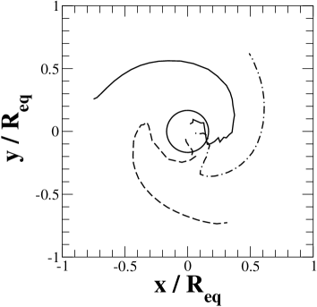
Figure 13: Phase-constant curve of perturbed radial velocity in the equatorial plane of an unstable $m=1$ mode for model I (see Table 1). The snapshot times are the same as that in Fig. 11. Solid circle denotes the corotation radius of the star. Note that the direction of rotation of background flow is counter-clockwise.

4 Canonical Angular Momentum to Diagnose Dynamical Instability

4.1 Introduction of canonical angular momentum

In order to diagnose the oscillations in a rotating fluid, we here introduce the canonical angular momentum following Friedman & Schutz (1978a). In the theory of adiabatic linear perturbations of a perfect fluid configuration with some symmetries, it is possible to introduce canonical conserved quantities associated with the symmetries. When we introduce Lagrangian displacement vector $\xi^{i}$, which is a vector connecting a perturbed fluid element to a corresponding non-perturbed one, the linearized perturbation equations are cast into a single second order differential equation for $\xi^{i}$ (Friedman & Schutz, 1978a);

$$A^{i}_{j}\partial_{t}^{2}\xi^{j}+B^{i}_{j}\partial_{t}\xi^{j}+C^{i}_{j}\xi^{j}=0.$$ (4.1)

Here the operators $A$ and $C$ are Hermitian, $B$ anti-Hermitian, respectively up to divergence term [see equations (32) to (34) in Friedman & Schutz (1978a) for the precise expressions], with respect to an inner product of displacements $\eta^{i}$ and $\xi^{i}$,

$$<\eta,\xi>\equiv\int{\eta_{i}}^{*}\xi^{i}dV=\int{\eta^{i}}^{*}\xi_{i}dV,$$ (4.2)

where $\eta^{*}$ means Hermite conjugate of $\eta$.

The master equation (4.1) is derived from the variational principle with an action

$$I=\int_{t_{1}}^{t_{2}}dt\int dV~{}{\cal L},$$ (4.3)

where Lagrangian density ${\cal L}$ is defined by

$${\cal L}:=\frac{1}{2}\left[(\partial_{t}{\xi^{*}_{i}})A^{i}_{j}(\partial_{t}{\xi}^{j})+(\partial_{t}{\xi^{*}_{i}})B^{i}_{j}\xi^{j}-\xi^{*}_{i}C^{i}_{j}\xi^{j}\right].$$ (4.4)

Applying Nöther’s theorem to this Lagrangian, we obtain canonical conserved quantities (Wald, 1984). In particular, if we have an axisymmetry in the background fluid, the corresponding Killing vector $\partial_{\varphi}$ produces a conserved current related to the angular momentum,

$${\cal J}^{\alpha}=\partial_{{}_{\varphi}}^{\alpha}{\cal L}-\frac{\partial{\cal L}}{\partial(\partial_{\alpha}\xi^{j})}\pounds_{{}_{\partial_{{}_{\varphi}}}}\xi^{j}-\frac{\partial{\cal L}}{\partial(\partial_{\alpha}\xi^{j*})}\pounds_{{}_{\partial_{{}_{\varphi}}}}\xi^{j*},$$ (4.5)

where $\partial_{\varphi}^{\alpha}$ is $\alpha-$component of vector $\partial_{\varphi}$, and $\pounds_{v}$ denotes Lie derivative along a vector $v$. Note that our variable $\xi^{i}$ is a complex vector field. The time component of this current is a canonical angular momentum density, while spacelike components are the flux density. In the rest of this section, let us follow Friedman & Schutz (1978a) to derive an explicit form of the canonical angular momentum.

A natural symplectic structure is introduced as an inner product of a field $\xi$ and its conjugate momentum density,

$$W(\eta,\xi):=\left<\eta,A(\partial_{t}{\xi})+\frac{1}{2}B\xi\right>-\left<A(\partial_{t}{\eta})+\frac{1}{2}B\eta,\xi\right>.$$ (4.6)

It is easy to find that this product is conserved using the master equation (4.1) and using the symmetric property of operators $A$, $B$, $C$ as

$$\partial_{t}W(\eta,\xi)=0,$$ (4.7)

where both $\eta^{i}$ and $\xi^{i}$ are solutions to the master equation (4.1). We obtain the canonical angular momentum of the system when the background fluid is axisymmetric (thus $A,B,C$ commute with $\partial_{\varphi}$),

$$J_{c}(\xi)=-\frac{1}{2}W(\partial_{\varphi}\xi,\xi),$$ (4.8)

which is a volume integral of the canonical angular momentum density defined by equation (4.5). From the definition, these conserved quantities are quadratic in the Lagrangian displacement vector.

These quantities, however, are ‘gauge-dependent’ in general. This means that we may find ‘trivial displacement’ vector $\zeta^{i}$ for any physical solution of the master equation (4.1). The trivial displacement is added to ‘physical’ solution $\xi^{i}$ to produce a different displacement, which corresponds to the same physical solution (i.e., it does not change Eulerian perturbation of physical quantities). The trivial defines a class of gauge transformation of the same physical solution, under which the canonical energy or momentum are generally not invariant. Thus a naive use of it to the stability problem of a fluid may lead to a wrong conclusion. Friedman & Schutz (1978a) showed that we can find a class of a physical solution to the master equation (4.1) called ‘canonical displacement’ orthogonal to the trivials, for which we have no contribution from the trivial displacement to the canonical quantities. Fortunately, in the case we are interested in (normal-mode problem with non-zero complex frequency), the displacement are always orthogonal to the trivials (Friedman & Schutz, 1978b).

Finally, we remark that the canonical energy or angular momentum of the dynamically unstable modes are zero. This is simply found if we are conscious of the existence of an imaginary part $\sigma_{I}$ in the eigenfrequency $\sigma$. Then the conservation equation of the product $W$ is written as

$$\partial_{t}W=2\sigma_{I}W=0,$$ (4.9)

and therefore $W=0$.

Figure 14: Distribution of the canonical angular momentum density for $m=1$ unstable mode. Plots are integrand of equation (4.16), $\varpi j_{c}(\varpi)$. Models (a) to (d) are the same as in Fig. 9. Vertical dashed lines mark the corotation radius of the mode.

Next we write down the explicit form of canonical angular momentum used in the following discussion.

$$J_{\rm c}(\xi) = -\frac{1}{2}\hat{W}(\partial_{\varphi}\xi,\xi)$$ (4.10)

$$= -\frac{1}{2}\left<\partial_{\varphi}\xi,A(\partial_{t}\xi)+\frac{1}{2}B\xi\right>$$

$$+\frac{1}{2}\left<A\partial_{\varphi}\partial_{t}\xi+\frac{1}{2}B\xi,\xi\right>.$$

Thus,

$$J_{\rm c}(\xi) = -\frac{1}{2}\int_{V}\partial_{\varphi}\xi_{i}^{*}A^{i}_{j}\partial_{t}\xi^{j}dV-\frac{1}{4}\int_{V}\partial_{\varphi}\xi_{i}^{*}B^{i}_{j}\partial_{t}\xi^{j}dV$$

$$+\frac{1}{2}\int_{V}A^{i}_{j}\partial_{t}\partial_{\varphi}\xi^{j*}\cdot\xi_{i}dV+\frac{1}{4}\int_{V}B^{i}_{j}\partial_{\varphi}\xi^{j*}\cdot\xi_{i}dV.$$

Note that since $A$, $B$, $C$ are defined in the background fluid whose physical quantities are purely real, they are ‘real’ quantities (although $B$ is anti-Hermite as an operator). As we are interested in a normal mode solution with harmonic dependence in $t$ and $\varphi$, the displacement vector can be written as

$$\xi=\xi_{0}(\varpi)e^{-i\sigma t+im\varphi},\quad\xi^{*}=\xi^{*}_{0}(\varpi)e^{i\sigma^{*}t-im\varphi}.$$ (4.12)

The first and third terms in equation (LABEL:def_J) are combined to produce

$$m\Re[\sigma]\int_{V}\rho|\xi|^{2}dV,$$ (4.13)

while the second and fourth are simplified as

$$\frac{im}{4}\int_{V}\left[\rho(\xi_{i}^{*}v^{k}\nabla_{k}\xi^{i}-\xi_{i}v^{k}\nabla_{k}\xi^{i*})+\nabla_{j}(\rho v^{j}\xi_{k}^{*}\xi^{k})\right]$$ (4.14)

$$-\frac{im}{4}\int_{V}\left[\rho(\xi_{i}v^{k}\nabla_{k}\xi^{i*}-\xi_{i}^{*}v^{k}\nabla_{k}\xi^{i})+\nabla_{j}(\rho v^{j}\xi_{k}^{*}\xi^{k})\right]$$

$$= -m\int_{V}\rho\cdot\Im\left[\xi_{i}^{*}v^{k}\nabla_{k}\xi^{i}\right]dV.$$

Note that $B$ is antisymmetric up to a divergence term which appears in the integral above. We have an exact cancellation to the contribution of $B$. As we are interested in the case with a circular flow as a background whose nonzero component of velocity is $v^{\varphi}=\Omega(\varpi)$, we can easily find that

$$\xi_{i}^{*}v^{k}\nabla_{k}\xi^{i}=im\Omega|\xi|^{2}-\varpi\Omega\xi^{\varpi*}\xi^{\varphi}+\varpi\Omega\xi^{\varphi*}\xi^{\varpi}.$$ (4.15)

Finally, we get the simple form of the canonical angular momentum $J_{\rm c}$ as

$$J_{\rm c}=m\int_{V}(\Re[\sigma]-m\Omega)\rho|\xi|^{2}dV-2m\int_{V}\rho\varpi\Omega\cdot\Im[\xi^{\varpi}\xi^{\varphi*}]dV.$$ (4.16)

4.2 Application to oscillations of a cylinder

We here present typical distribution of the canonical angular momentum in the cylinder model. The absolute amplitude of the plotted function here has no significance, since a linear eigenfunction can be scaled arbitrarily.

In Fig. 14, we plot the integrand of canonical angular momentum, defined from equation (4.16) as

$$\varpi j_{\rm c}(\varpi)=m(\Re[\sigma]-m\Omega)\rho|\xi|^{2}-2m\rho\varpi\Omega\cdot\Im[\xi^{\varpi}\xi^{\varphi*}],$$ (4.17)

for unstable $m=1$ mode. Here, $j_{c}$ is the canonical angular momentum density. Note that an integral in the entire cylinder is zero for these cases. The features of the canonical angular momentum distribution for $m=1$ unstable modes are,

1. It changes sign around corotation radius $\varpi_{\rm crt}$.

2. It is positive for $\varpi<\varpi_{\rm crt}$, while negative for $\varpi>\varpi_{\rm crt}$.

The feature 1 is remarkable and suggests us that the instability is related to the corotation. The feature has a clear contrast for a stable mode (Fig. 15). The canonical angular momentum is either positive or negative definite, and it does not change its sign. Note that the former is the case when the pattern speed of mode is faster than the rotation of cylinder everywhere, while the latter is the opposite. This feature is expected from the equation (4.16), if the first term is dominant. In such case, the sign of $\Re[\sigma]-m\Omega(\varpi)$ determines the sign of the canonical angular momentum. This simple interpretation, however, does not hold for the dynamically unstable mode. As it is shown in the feature 2 above, we have a positive canonical angular momentum inside the corotation, which is opposite to the sign of $\sigma-\Omega(\varpi)$ for $0\leq\varpi<\varpi_{\rm crt}$.

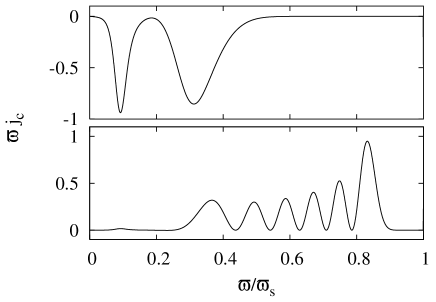
Figure 15: Distribution of the canonical angular momentum density for $m=1$ stable modes. Plots are integrand of equation (4.16), $\varpi j_{c}(\varpi)$. The parameters of top and bottom panels correspond to (b)-s1 and (b)-s2 in Table 2. The model (b)-s1 satisfies $\sigma-\Omega(\varpi)<0$, while the model (b)-s2 satisfies $\sigma-\Omega(\varpi)>0$ throughout the fluid.

In Fig. 16, we show an example of canonical angular momentum distribution for $m=2$ unstable mode of differentially rotating cylinder, which may be compared with the low $T/|W|$ bar instability of Shibata et al. (2002, 2003). We did not find $m=2$ unstable modes for the same parameters as in the case of $m=1$ instability. The features at the corotation radius, however, are the same as in $m=1$ instability.

It is interesting to see how the profile of the canonical angular momentum changes when we consider the classical bar instability with uniform rotation. Unfortunately the bar mode of uniformly rotating cylinder has a neutral stability point at the breakup limit (Luyten, 1990). We instead looked at $m=2$ instability of uniformly rotating, incompressible Bardeen disk (Bardeen, 1975) and the classical bar instability of Maclaurin spheroid (see Appendix A for these computation). These are actually more suitable for comparison to differentially rotating spheroidal model, which we present in the following section. For both of the models we have analytic expressions of oscillation modes [Schutz & Bowen (1983) for a Bardeen disk and Chandrasekhar (1969) for Maclaurin spheroid]. It is remarkable that the canonical angular momentum density is zero everywhere (which ensures that the total canonical angular momentum vanishes). This is in a clear contrast with the $m=2$ instability in the cylinder with highly differential rotation.

Figure 16: Distribution of canonical angular momentum density for $m=2$ unstable modes (model (e) in Table 2). Plots are integrand of equation (4.16), $\varpi j_{c}(\varpi)$. The vertical dashed line marks the corotation radius.

4.3 Differentially rotating star

We here present the application of the canonical angular momentum to our hydrodynamics results. Following three assumptions are made to adopt our hydrodynamic results of dynamical instability (for both $m=1$ and $m=2$) to the perturbative approach;

1. All physical quantities is in coherent oscillation of growing mode.

2. For each model, a growing mode with single $m$ is dominant.

3. The motion of $z$-direction does not contribute to the instability.

From assumption 1 we introduce a complex frequency $\sigma$ that represents the same growing mode $m$. Therefore all physical quantities $f(t)$ that have a time dependence should satisfy

$$f(t)=f_{1}\exp(-i\sigma t),$$ (4.18)

where $\sigma=\sigma_{\rm R}+i\sigma_{\rm I}$, $f_{1}$ is a complex quantity. Note that $\sigma_{\rm R}$ and $\sigma_{\rm I}$ are real quantities.

The assumption 2 comes from the fact that single $m$ mode has a dominant contribution to the dynamical instability in the diagnostics (Fig. 1). Therefore all physical quantity $f(\varpi,\varphi)$ that have a dependence of azimuthal angle should satisfy

$$f(\varpi,\varphi)=f(\varpi)\exp(im\varphi),$$ (4.19)

where

$$f(\varpi)=\frac{1}{2\pi}\int_{0}^{2\pi}d\varphi~{}f(\varpi,\varphi)\exp(-im\varphi).$$ (4.20)

From the velocity snapshots in the meridional plane (Fig. 5), the motion of the fluid along the rotation axis does not have a significant contribution to the instability. Therefore we can neglect the $z$-dependence in the function (assumption 3) as

$$f(\varpi,z)=f(\varpi).$$ (4.21)

From the three assumptions, we determine the frequency from the dipole and quadrupole diagnostics as

$$D(t) = \frac{1}{M}\int dv\rho(t,\varpi,\varphi,z)\exp(i\varphi)$$ (4.22)

$$= \exp(-i\sigma t)\frac{1}{M}\int d\varpi 2\pi\varpi\rho(\varpi),$$

$$Q(t) = \frac{1}{M}\int dv\rho(t,\varpi,\varphi,z)\exp(2i\varphi)$$ (4.23)

$$= \exp(-i\sigma t)\frac{1}{M}\int d\varpi 2\pi\varpi\rho(\varpi).$$

With the formulae above, we extract the complex frequency by fitting evolutions of dominant diagnostics for each cases.

Note that we averaged the frequency in the early stage of the evolution, since the real part of the frequency is almost the same. Note also that $D(0)\not=0$ and $Q(0)\not=0$ since we put $m=1$ and $m=2$ density perturbation at $t=0$ (equation 2.9) to initiate $m=1$ or $m=2$ dynamical instability.

Table 3: Eigenfrequency and the corotation radius of three differentially rotating stars

Model	$\sigma$ $[\Omega_{\rm c}]$	$\varpi_{\rm crt}$ $[R_{\rm eq}]$
I	$0.590+0.0896i$	$0.167$
II	$0.284+0.0121i$	$0.492$
III	$0.757+0.200i$	—

We summarize the corotation radius and the complex frequency in Table 3 from Fig. 1. Eulerian perturbed velocity is defined as

$$\partial_{t}v^{i}(t,\varpi,\varphi)=v^{i}(t,\varpi,\varphi)-v^{i}_{\rm eq}(\varpi),$$ (4.24)

where $v^{i}(t,\varpi,\varphi)$ is the velocity at $t$, $v^{i}_{\rm eq}(\varpi)$ is the velocity at equilibrium, respectively. Following assumption 2, we find,

$$\partial_{t}v^{i}(t,\varpi)=\frac{1}{2\pi}\int_{0}^{2\pi}d\varphi~{}\partial_{t}v^{i}(t,\varpi,\varphi)\exp(-im\varphi).$$ (4.25)

The Lagrangian displacement $\xi^{i}$ should satisfy the following differential equation:

$$\partial_{t}\xi^{i}=\partial_{t}v^{i}+\xi^{k}\partial_{k}v^{i}_{\rm eq}-v^{k}_{\rm eq}\partial_{k}\xi^{i}.$$ (4.26)

Using the three assumptions, $\varpi$ and $\varphi$ component of the Lagrangian displacement should be written as

$$\xi^{\varpi} = \frac{i\partial_{t}v^{\varpi}}{\sigma-m\Omega_{\rm eq}},$$ (4.27)

$$\xi^{\varphi} = \frac{i\partial_{t}v^{\varphi}}{\sigma-m\Omega_{\rm eq}}-\frac{(\partial_{t}v^{\varpi})(\partial_{\varpi}\Omega_{\rm eq})}{(\sigma-m\Omega_{\rm eq})^{2}},$$ (4.28)

where $\Omega_{\rm eq}$ denotes the angular velocity at equilibrium.

Using the Lagrangian displacement extracted by the formula above, we compute the canonical angular momentum density defined as an integrand of the canonical angular momentum in equation (4.16) as

$$J_{\rm c}=\int d\varpi~{}\varpi j_{\rm c}(\varpi),$$ (4.29)

where

$$\varpi j_{\rm c}(\varpi)=m(\Re[\sigma]-m\Omega)\rho|\xi|^{2}-2m\rho\varpi\Omega\cdot\Im[\xi^{\varpi}\xi^{\varphi*}].$$ (4.30)

Note that we have used the assumptions 1 – 3 to compute the canonical angular momentum density.

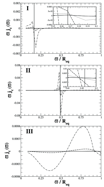
Figure 17: Snapshots of the canonical angular momentum distribution $\varpi j_{\rm c}(\varpi)$ in the equatorial plane for three differentially rotating stars (see Table 1). Solid, dotted, dashed, and dash-dotted line represents the time $t/P_{\rm c}=$(3.47, 6.93, 10.40, 13.86) for model I, $t/P_{\rm c}=$(45.68, 56.43, 67.18, 77.97) for model II, and $t/P_{\rm c}=$(1.10, 2.19, 3.29, 4.39) for model III, respectively. Note that vertical line in panels I and II denotes the corotation radius of the star (model III does not have a corotation radius). We also enlarged the figure around the corotation radius for panels I and II, which is presented in the right upper part of each panel. Although our method of determining the corotation radius is not precise, we clearly find that the distribution significantly changes around the corotation radius.

We show the snapshots of canonical angular momentum density in Fig. 17. Since we determine the corotation radius using the extracted eigenfrequency and the angular velocity profile at equilibrium, the radius does not change throughout the evolution. For low $T/|W|$ dynamical instability, the distribution of the canonical angular momentum drastically changes its sign around the corotation radius, and the maximum amount of canonical angular momentum density increases at the early stage of evolution. This means that the angular momentum flows inside the corotation radius in the evolution. On the other hand, for high $T/|W|$ dynamical instability (the bottom panel of Fig. 17), which may be regarded as a classical bar instability modified by differential rotation, the distribution of the canonical angular momentum is smooth and with no particular feature.

Note that the amplitude of $\varpi j_{c}$ is orders of magnitude smaller than those in the corotating cases in top and middle panels of Fig. 17. Contrary to the linear perturbation analysis in Section 4.2, the amplitude here is not scale free and the relative amplitude has a physical meaning. Thus the smallness of it for model III suggest that it should be exactly zero everywhere in the limit of linearized oscillation. The deviation from zero may come from the imperfect assumption of linearized oscillation, that is made here to extract oscillation frequency and Lagrangian displacement vector.

From these different behaviours of the distribution of the canonical angular momentum, we find that the mechanisms working in the low $T/|W|$ instabilities and the classical bar instability may be quite different, i.e., in the former the corotation resonance of modes are essential, while the instability is global in the latter case.

5 Summary and Discussion

We have studied the nature of three different types of dynamical instability in differentially rotating stars both in linear eigenmode analysis and in hydrodynamic simulation using canonical angular momentum distribution.

We have found that the low $T/|W|$ dynamical instability occurs around the corotation radius of the star by investigating the distribution of the canonical angular momentum. We have also found by investigating the canonical angular momentum that the instability grows through the inflow of the angular momentum inside the corotation radius. The feature also holds for the dynamical bar instability in low $T/|W|$, which is in clear contrast to that of classical dynamical bar instability in high $T/|W|$. Therefore the existence of corotation point inside the star plays a significant role of exciting one-armed spiral mode and bar mode dynamically in low $T/|W|$. However, we made our statement from the behaviour of the canonical angular momentum, the statement holds only in a sense of necessary condition. In order to understand the physical mechanism of the low $T/|W|$ dynamical instability, we need another tool and it will be the next step of this study.

The feature of gravitational waves generated from these instabilities are also compared. Quasi-periodic gravitational waves emitted by stars with $m=1$ instabilities have smaller amplitudes than those emitted by stars unstable to the $m=2$ bar mode. For $m=1$ modes, the gravitational radiation is emitted not directly by the primary mode itself, but by the $m=2$ secondary harmonic which is simultaneously excited. Possibly this $m=2$ oscillation is generated through a quadratic nonlinear selfcoupling of $m=1$ eigenmode. Remarkably the precedent studies (Centrella et al., 2001; Saijo et al., 2003) found that the pattern speed of $m=2$ mode is almost the same as that of $m=1$ mode, which suggest the former is the harmonic of the latter. Unlike the case for bar-unstable stars, the gravitational wave signal does not persist for many periods, but instead is damped fairly rapidly. We have not understood this remarkable difference between $m=1$ and $m=2$ unstable cases. One of the possibility may be that the unstable $m=1$ eigenmode tends to couple to higher and higher $m$ modes (which are not necessarily unstable and could be in the continuous spectrum) and pump its energy to them in a cascade way. However, we have not found the feature that prevents $m=2$ mode from this cascade dissipation.

Another possibility is that the spiral pattern formed in $m=1$ instability redistributes the angular momentum of the original unstable flow, so that the flow is quickly stabilized. Inside the corotation radius, the background flow is faster than the pattern, while it is slower outside. A similar mechanism to Landau damping in plasma wave which transfer the momentum of wave to background flow may work at the spiral pattern. The pattern may decelerate the background flow inside the corotation and accelerate it outside the corotation, which may change the unstable flow profile to stable one. As we do not see a spiral pattern forming in the low $T/|W|$ bar instability, it may eludes this damping process.

Appendix A Canonical angular momentum of classical bar instability

In this appendix we evaluate the angular momentum density of bar instability in Bardeen disk and in Maclaurin spheroid. This quantity is defined in the cylindrical coordinate as

$$j_{c}(\varpi) = m\Re[s]\rho|\xi|^{2}-2m\Omega\rho~{}\Im[\xi^{\varpi}\cdot\xi^{\varphi*}]$$ (1.1)

$$= \frac{m\rho}{|s|^{2}}\left(\Re[s]|\delta v|^{2}+2\Omega~{}\Im\left[\delta v^{\varpi}\cdot\delta v^{\varphi*}\right]\right),$$ (1.2)

where $s=\sigma-m\Omega$ is the frequency of the mode observed in corotating frame of the fluid. The components of Lagrangian displacement $\xi$ and Eulerian velocity $\delta v$ are written in the local orthonormal frame.

A.1 Bardeen disk

Bardeen (1975) analytically constructed a self-gravitating ‘warm’ disk with finite thickness by finding corrections to an infinitesimally thin disk from which he started his approximation. Perturbation of a Bardeen disk is studied in Schutz & Bowen (1983). Here, we follow their definitions and notations. Velocity perturbation is written with two potential functions $\alpha$ and $\beta$ as

$$\delta v=-i\nabla\alpha-\nabla\times(\beta e_{z}),$$ (1.3)

where $e_{z}$ is the unit vector in $z$-direction. Introducing $\eta=\sqrt{1-({\varpi}/{R})^{2}}$ in terms of cylindrical radial coordinate $\varpi$, the general perturbation can be expanded by Legendre polynomials as

$$\alpha=\sum_{l=0}^{\infty}\sum_{m=-\infty}^{\infty}\alpha_{l}^{m}P_{2l+m}^{m}(\eta)e^{im\varphi}.$$ (1.4)

Master equations (equations (3.1) and (3.4) in Schutz & Bowen (1983)) for perturbation can be decomposed into those for each $l$ and $m$. The bar mode is $l=0$, $m=0$ case. From equations (3.13) to (3.15) of Schutz & Bowen (1983), we get a simple eigenvalue equation

$$s^{2}-2\Omega s+\frac{3}{2}-\frac{16\mu}{\pi}=0,$$ (1.5)

where $\Omega$ is the angular velocity of disk

$$\Omega=\sqrt{1-\frac{8\mu}{\pi}},$$ (1.6)

while $s$ is a mode frequency observed in a corotating frame with disk. Both of them are normalized by $\Omega_{\rm cld}$, an angular frequency of cold disk. $\mu$ is called ‘aspect ratio’ parameter (equation (2.18) in Schutz & Bowen (1983)). When this parameter is smaller than ${\pi}/{16}$, one of the modes above becomes dynamically unstable. The corresponding radial eigenfunctions are written as

$$\alpha_{2}^{2} = K\left(1+\frac{8\Gamma}{s(s+2\Omega)}\right)P_{2}^{2}({\eta}),$$ (1.7)

$$\beta_{2}^{2} = K\left(1-\frac{8\Gamma}{s(s+2\Omega)}\right)P_{2}^{2}({\eta}),$$ (1.8)

where

$$\Gamma=\frac{3}{16}-\frac{2\mu}{\pi}.$$ (1.9)

Using $\alpha_{2}^{2}$ and $\beta_{2}^{2}$,Eulerian perturbation of velocity for bar mode is written as

$$\delta v^{\varpi} = -i\left(\frac{d}{d\varpi}\alpha_{2}^{2}+\frac{2}{\varpi}\beta_{2}^{2}\right)=-6iK\varpi,$$ (1.10)

$$\delta v^{\varphi} = \frac{d}{d\varpi}\beta_{2}^{2}+\frac{2}{r}\alpha_{2}^{2}=6K\varpi,$$ (1.11)

where we used the definition of $\eta$. With bearing in mind that the real part of $s$ is $\Omega$, equation (1.2) gives that $j_{c}$ is 0.

A.2 Maclaurin spheroid

For the bar mode of Maclaurin spheroid, we have an analytical expression of Lagrangian displacement,

$$\xi^{x}=k\varpi e^{\pm i\varphi},~{}\xi^{y}=k\varpi e^{\pm i(\varphi+\frac{\pi}{2})},~{}\xi^{z}=0,$$ (1.12)

in Cartesian components (Chandrasekhar, 1969). Here $k$ is a constant. It is straightforward to see that the corresponding components in cylindrical coordinate are

$$\xi^{\varpi}=k\varpi e^{\pm 2i\varphi},~{}\xi^{\varphi}=\pm ke^{\pm 2i\varphi},~{}\xi^{z}=0.$$ (1.13)

$\xi^{\varphi}$ is defined with respect to coordinate base vector $\partial/\partial\varphi$. From equation (1.1) with the fact that real part of frequency of unstable bar mode is $\Omega$, we easily see that $j_{\rm c}$ vanishes everywhere.

References

- Acheson (1976) Acheson D. J., 1976, J. Fluid Mech., 77, 433
- Balbinski (1985) Balbinski E., 1985, MNRAS, 216, 897
- Bardeen (1975) Bardeen J. M., 1975, in Hayli A., eds., Proc. IAU Symp. 69, Dynamics of Stellar Systems. Reidel, Dordrecht, p. 297
- Blaes (1985a) Blaes O. M., 1985a, MNRAS, 212, 37
- Blaes (1985b) Blaes O. M., 1985b, MNRAS, 216, 553
- Blaes & Glatzel (1986) Blaes O. M., Glatzel W., 1986, MNRAS, 220, 253
- Cook et al. (2003) Cook J. N., Shapiro S. L., Stephens B. C., 2003, ApJ, 599, 1272
- Centrella et al. (2001) Centrella J. M., New K. C. B., Lowe L. L., Brown, J. D., 2001, ApJ, 550, L193
- Chandrasekhar (1969) Chandrasekhar S., 1969, Ellipsoidal Figures of Equilibrium. Yale Univ. Press, New York, Chap. 5, Sec. 33
- Christodoulou & Narayan (1992) Christodoulou D. M., Narayan R., 1992, ApJ, 388, 451
- Drury (1985) Drury, L. O’C., 1985, MNRAS, 217, 821
- Duez et al. (2004) Duez M. D., Shapiro S. L., Yo H.-J., 2004, PRD 69, 104016
- Durisen et al. (1986) Durisen R. H., Gingold R. A., Tohline J. E., Boss A. P., 1986, ApJ, 305, 281
- Friedman & Schutz (1978a) Friedman J. L., Schutz B. F., 1978a, ApJ, 221, 937
- Friedman & Schutz (1978b) Friedman J. L., Schutz B. F., 1978b, ApJ, 222, 281
- Glatzel (1987a) Glatzel W., 1987a, MNRAS, 225, 227
- Glatzel (1987b) Glatzel W., 1987b, MNRAS, 228, 77
- Goldreich et al. (1986) Goldreich P., Goodman J., Narayan R., 1986, MNRAS, 221, 339
- Goodman & Narayan (1988) Goodman J., Narayan R., 1988, MNRAS, 231, 97
- Hachisu (1986) Hachisu I., 1986, ApJS, 61, 479
- Houser & Centrella (1996) Houser J. L., Centrella J. M., 1996, PRD, 54, 7278
- Houser et al. (1994) Houser J. L., Centrella J. M., Smith S. C., 1994, PRL 72, 1314
- Ishibashi & Ando (1985) Ishibashi S., Ando H., 1985, PASJ, 37, 97
- Ishibashi & Ando (1986) Ishibashi S., Ando H., 1986, PASJ, 38, 295
- Kojima (1986) Kojima Y., 1986, Prog. Theor. Phys., 75, 251
- Kojima (1989) Kojima Y., 1989, MNRAS, 236, 589
- Luyten (1988) Luyten P., 1988, Ap&SS, 141, 27
- Luyten (1989) Luyten P., 1989, Ap&SS, 153, 13
- Luyten (1990) Luyten P., 1990, MNRAS, 242, 447
- Narayan et al. (1987) Narayan R., Goldreich P., Goodman J., 1987, MNRAS, 228, 1
- Misner et al. (1973) Misner C. W., Thorne K. S., Wheeler J. A., 1973, Gravitation. Freeman, New York, Chap. 36.10
- New et al. (2000) New K. C. B., Centrella J. M., Tohline J. E., 2000, PRD, 62, 064019
- Ostriker (1965) Ostriker J., 1965, ApJS, 11, 167
- Ott et al. (2005) Ott C. D., Ou S., Tohline J. E., Burrows A., 2005, ApJL, 625, 119
- Papaloizou & Pringle (1984) Papaloizou J. C. B., Pringle J. E., 1984, MNRAS, 208, 721
- Papaloizou & Pringle (1985) Papaloizou J. C. B., Pringle J. E., 1985, MNRAS, 213, 799
- Papaloizou & Pringle (1987) Papaloizou J. C. B., Pringle J. E., 1987, MNRAS, 225, 267
- Pickett et al. (1996) Pickett B. K., Durisen R. H., Davis G. A., 1996, ApJ, 458, 714
- Robe (1979) Robe H., 1979, A&A, 75, 14
- Ruoff & Kokkotas (2001) Ruoff J., Kokkotas K. D., 2001, MNRAS, 328, 678
- Saijo (2005) Saijo M., 2005, PRD, 71, 104038
- Saijo et al. (2001) Saijo M., Shibata M., Baumgarte T. W., Shapiro S. L., 2001, ApJ, 548, 919
- Saijo et al. (2003) Saijo M., Baumgarte T. W., Shapiro S. L., 2003, ApJ, 595, 352
- Schutz & Bowen (1983) Schutz B. F., Bowen A. M., 1983, MNRAS, 202, 867
- Shapiro & Teukolsky (1983) Shapiro S. L., Teukolsky S. A., 1983, Black Holes, White Dwarfs, and Neutron Stars. John Wiley and Sons, New York, Chap. 7.5
- Shibata et al. (2000) Shibata M., Baumgarte T. W., Shapiro S. L., 2000, ApJ, 542, 453
- Shibata et al. (2002) Shibata M., Karino S., Eriguchi Y., 2002, MNRAS, 334, L27
- Shibata et al. (2003) Shibata M., Karino S., Eriguchi Y., 2003, MNRAS, 343, 619
- Shibata & Sekiguchi (2005) Shibata M., Sekiguchi Y.-I., 2005, PRD, 71, 024014
- Shu (1992) Shu F. H., 1992, The Physics of Astrophysics: Volume II Gas Dynamics. University Science Book, Mill Valley, California, Chapters 11, 12
- Smith et al. (1995) Smith S. C., Houser J. L., Centrella J. M., 1995, ApJ, 458, 236
- Stix (1992) Stix T. H., 1992, Waves in Plasmas. American Institute of Physics, New York, Chap. 8
- Tassoul (1978) Tassoul J.-L., 1978, Theory of Rotating Stars. Princeton Univ. Press., Princeton, Chap. 10
- Tohline et al. (1985) Tohline J. E., Durisen R. H., McCollough M., 1985, ApJ, 298, 220
- Tohline & Hachisu (1990) Tohline J. E., Hachisu I., 1990, ApJ, 361, 394
- Toman et al. (1998) Toman J., Imamura J. N., Pickett B. J., Durisen R. H., 1998, ApJ, 497, 370
- Wald (1984) Wald R. M., 1984, General Relativity. Univ. Chicago Press, Chicago, Appendix E.
- Watts et al. (2003) Watts A. L., Andersson N., Beyer H., Schutz B. F., 2003, MNRAS, 342, 1156
- Watts et al. (2005) Watts A. L., Andersson N., Jones D. I., 2005, ApJL, 618, 37
- Williams & Tohline (1988) Williams H. A., Tohline J. E., 1988, ApJ, 334, 449
- Zink et al. (2005) Zink B., Stergioulas N., Hawke I., Ott C. D., Schnetter E., Müller E., 2005, preprint (gr-qc/0501080)