A new reduction of the raw Hipparcos data

We present an outline of a new reduction of the Hipparcos astrometric data, the justifications of which are described in the accompanying paper. The emphasis is on those aspects of the data analysis that are fundamentally different from the ones used for the catalogue published in 1997. The new reduction uses a dynamical modelling of the satellite’s attitude. It incorporates provisions for scan-phase discontinuities and hits, most of which have now been identified. Solutions for the final along-scan attitude (the reconstruction of the satellite’s scan phase), the abscissa corrections and the instrument model, originally solved simultaneously in the great-circle solution, are now de-coupled. This is made possible by starting the solution iterations with the astrometric data from the published catalogue. The de-coupling removes instabilities that affected great-circle solutions for short data sets in the published data. The modelling-noise reduction implies smaller systematic errors, which is reflected in a reduction of the abscissa-error correlations by about a factor 40. Special care is taken to ensure that measurements from both fields of view contribute significantly to the along-scan attitude solution. This improves the overall connectivity of the data and rigidity of the reconstructed sky, which is of critical importance to the reliability of the astrometric data. The changes in the reduction process and the improved understanding of the dynamics of the satellite result in considerable formal-error reductions for stars brighter than 8th magnitude.

1 Introduction

Although the Hipparcos mission (ESA 1997; Perryman et al. 1997; van Leeuwen 1997; Kovalevsky 1998) finished more than ten, and the reductions some eight, years ago, there are still aspects of the mission that are only now becoming fully understood. These aspects mostly concern peculiarities of the rotation rates of the satellite (and in particular the scan velocity), and methods used to reconstruct these rates and the resulting angular displacements as a function of time. This process, referred to as the attitude reconstruction, ultimately provides the reference frame against which the scientific products of the mission are measured: time-resolved positional information on 118 000 pre-selected stars. The accuracy of the attitude reconstruction is therefore a determining factor in the overall quality of the astrometric data produced by the mission, and, as was stated in the accompanying paper, this process is to a large extent determined by our understanding of the rotational motions of the spacecraft. It is the progress in this understanding that has played a major role in the new reduction.

Despite a serious problem with the orbit due to a failure of the apogee boost motor (see Volume 2 of ESA 1997; Dalla Torre & van Leeuwen 2003), and the resulting solution instabilities and radiation damage, Hipparcos produced results well exceeding the expectations set for the nominal mission. This was confirmed by a wide range of statistical tests on the final data (Arenou et al. 1995; Lindegren 1995). At the time of the publication (ESA 1997), it was therefore generally assumed that a complete re-reduction of these data would never be attempted or even be needed: it seemed that the best possible results had already been obtained by careful merging of the results from the two independent reduction chains, FAST (Kovalevsky et al. 1992) and NDAC (Lindegren et al. 1992). It was envisaged that any further improvements would be done using the published intermediate astrometric data, the abscissa residuals that were used to derive the astrometric parameters for the program stars (van Leeuwen & Evans 1998).

Full-sky survey missions like Hipparcos are self-calibrating: their scientific products are also used for defining the instrument characteristics. For Hipparcos, the reconstruction of the along-scan attitude uses the same measurements that form the input for the astrometric-parameter determinations. These two reconstructions are separated in two ways: measurements at different epochs allow the recognition of displacements due to proper motions, while simultaneous measurements in the two fields of view (with different along-scan parallax-factors) allow ultimately for the recognition of displacements due to parallaxes. However, the process of separation is non-linear and the Hipparcos catalogue can therefore only be obtained as the result of a sequence of iterations through the mission data. The present study can in that sense be understood as a further and probably final set of iterations. Starting these iterations with the data as presented in the published catalogue for starting values, allows simplifications in the reductions, which remove potential instabilities from the solutions. Furthermore, modern computers make a much faster reduction of the data possible, which allows the iterations to take place that are necessary to reach photon-count limits on the accuracies for stars as bright as magnitude 3 to 4, requiring an accuracy for the reference frame of better than 0.1 mas.

Since the publication in 1997 doubts have been raised about some of the results derived from the catalogue data, most noticeably the distances of a few open clusters. The astrometric data for open clusters are based on combined results from the cluster members, which, instead of being solved for as individual stars, are solved together for a single cluster parallax and proper motion (van Leeuwen & Evans 1998; van Leeuwen 1999; Robichon et al. 1999). The precision of a cluster parallax is therefore generally higher than that of individual stars, and can indicate in more detail possible problems in the catalogue. In particular the difference between the expected and observed parallax of the Pleiades cluster has been used as an indication that in some difficult areas of the sky the mechanisms of the data reductions may not always have been optimal (Pinsonneault et al. 1998, 2000, 2003; Soderblom et al. 1998; Narayanan & Gould 1999; Reid 1999). A likely cause of these problems was identified by Makarov (2002) and van Leeuwen (2005) as due to a problem in the along-scan attitude reconstruction in the presence of high-density star fields. By not incorporating a correction for the large weight discrepancies that could occur under these conditions, the along-scan attitude would be dominated by data from one field of view only, and the astrometry for such a high-density field could become (partly) disconnected from the rest of the catalogue. This issue will be referred to as the connectivity of the data. Good connectivity is one of the two fundamental conditions for an astrometric mission of the type of Hipparcos. The other is a stability requirement on the basic angle between the two fields of view.

The current study was not initiated with the idea or intention to re-reduce the Hipparcos data. Instead, between 1998 and 2003, we undertook a study on the dynamics of the satellite as derived from the reconstructed attitude files obtained over the mission (Fantino 2000; Fantino & van Leeuwen 2003). The aim was to try to understand the torques acting on the satellite well enough to use that information in the reconstruction of the attitude. The uniquely-high accuracy level of the Hipparcos attitude reconstruction exposes details in external torques never seen before. However, experiments with the reconstructed attitude for the NDAC reductions used in the published data showed that, when interpreted as rotational velocities and accelerations, details of the reconstructed attitude generally contradicted what could be expected for a freely moving rigid body. These violations, which are the equivalent of modelling errors, reflect in correlations between the abscissa residuals, for which the measurements are obtained relative to the reconstructed attitude (van Leeuwen & Evans 1998). We therefore set out to test the hypothesis that by using a dynamical model for the satellite attitude, a more reliable reconstruction could be obtained. However, testing this hypothesis required re-reducing a large fraction of the Hipparcos raw data. The testing exposed a number of defects in the data that could be repaired, such as the scan-phase jumps and external hits described in the accompanying paper. Once these defects were taken care off, the attitude noise and error correlations started to drop dramatically. At the same time the importance of connectivity in producing absolute parallaxes became much better understood. With all that information in hand, the availability of the raw data and a new data analysis package, we were left with no other choice than a complete re-reduction of the raw data. As the stars that are most affected (those brighter than 8^th magnitude) include for example many open cluster members and a number of Cepheids, it was judged that a new reduction is more than just a technical or data analysis exercise: it is also highly desirable from an astrophysical point of view.

In the original reductions, between 1989 and 1997, it took a considerable manpower effort, and six to eight months, to process just once the entire data stream with the then available hardware. Handling the Hipparcos data has become much simpler over the years. The data for the mission had originally been delivered on 9-track 6250 bpi magnetic tapes, about 1100 in total. In the NDAC consortium these had been converted to an early version of the optical disk, using a total of about 160 disks. With these disks some random access to the data was possible all through the mission. In 1999 these disks were replaced by a CD-ROM archive (180 disks), and early 2003 that archive was converted to 24 DVDs. The data that used to occupy the space of almost an entire office is now kept in the drawer of a desk. With new software (written in C⁺⁺, and including extensive display facilities) and new hardware we are now able to go once through the entire data stream in three weeks, and for further iterations in about three to four days.

We present an overview of the new reduction in Section 2, with the emphasis on where the new approach is different from the earlier analysis. The attitude reconstruction method as used in the new reduction is described in Section 3. The statistics of the new analysis, demonstrating the internal consistency, are described in Section 4. The derivation of the astrometric parameters is described in Section 5. Suggestions for external tests, to verify formal errors and general conformity of the new results, are presented in Section 6, and our conclusions in Section 7.

This, and the accompanying paper, form the culmination of more than 7 years of investigations, testing, checking and processing. During that time various people have given advice and on occasion put us back on the right track again. In particular advice from Lennart Lindegren, at some critical stages of the development, has been highly valuable. Discussions we had on intermediate results with Michael Perryman, Rudolf Le Poole, Dafydd Evans, Frédéric Arenou, Ulrich Bastian and François Mignard are also much appreciated.

2 Summary of the new reduction

The new reduction differs from the earlier reductions by FAST and NDAC in two major aspects, both of which concern the reconstruction of the along-scan attitude. The first aspect is the dynamical modelling of the attitude, in which the underlying torques rather than the pointing variations are modelled, and which constrains the movements of the satellite to the physics of a freely rotating rigid body. It was hoped that these physical constraints would reduce systematic errors in the attitude. The improved understanding of the movements of the satellite gained from applying the dynamic modelling would also be of benefit to the attitude modelling.

The second aspect is the de-coupling of the three parameter sets that were, in the original reductions, solved simultaneously in a process referred to as the great-circle reduction (van der Marel 1988; van der Marel & Petersen 1992). These constituted the corrections to the abscissae, the along-scan attitude and the instrument parameters. The de-coupling has become possible as the a priori astrometric parameters (the predicted star positions for a given circle) are obtained from the published catalogue and have relatively low levels of largely white noise. This is quite different from the starting positions provided by the Input Catalogue (ESA 1989, 1992) used in the original reduction. The de-coupling has many advantages:

• it prevents the occurrence of instabilities that characterise short data sets in the original reduction (see accompanying paper);

• it no longer uses projection on a reference great circle, which could introduce additional noise; the sensitivity to errors in the reconstruction of the spin-axis position is therefore much reduced;

• the data now available for determining astrometric parameters are field transits rather than the combined transit data over an orbit of the satellite; field transits have better defined statistical properties than the combined transits for an orbit, referred to as “orbit transits”, and allow for improved detection and elimination of disturbed measurements and small-scale grid distortions;

• the resolution of data used in the three processes can now be adjusted to the specific requirements, providing in particular an improvement in the detection of disturbances like scan-phase jumps and satellite hits;

• it is now possible to apply adjustments for strong weight discrepancies between the data in the two fields of view, which is needed to improve the rigidity of the reconstructed catalogue.

Like the original reductions, the new reduction is a block-iterative adjustment. The starting conditions for the new reduction, however, reduced the systematic errors in the a priori astrometry to an insignificant level, which made it possible to sub-divide one block of the original reductions into three independently-solved blocks, greatly improving the stability of the solutions.

With these changes in place, and a completely re-written software package, the statistics of the intermediate reduction results can be followed in detail and used to detect at an early stage any problems in the data. Improvements are also made by preserving more information in the intermediate data products, such as the offset of the sensitive area of the main detector (the instantaneous field of view or IFOV), and the total photon count that contributed to an observation. The nominal signal modulation parameter $M1$ is also preserved (see the accompanying paper). The latter two parameters should provide a reliable handle on formal errors from the first reductions to the final astrometric parameter determinations.

Some minor changes are applied to the instrument-parameter solution. The basic angle correction is also included in the corrections for the along-scan attitude as the systematic difference for the corrections in the two fields of view. This allows for the occasional correction for basic-angle drifts. Chromaticity terms, which originally were entered only in the sphere solution, can now be solved directly as part of the instrument parameters. Finally, in the sphere solution corrections are also very small. This process too is therefore treated in a differential manner: after solving for the new astrometric parameters the remaining residuals are used to determine the corrections for the reference phases of each circle as well as residual colour dependences. Small-scale distortions as a function of the transit ordinate can now be investigated too. Provisions for 6^th harmonic residual modulations are no longer needed, as these originally resulted from instabilities in the great-circle reductions.

The new reduction includes information from the second harmonic of the modulated signals from the main grid, similar to that done by the FAST consortium. There is, however, a difference in the weights assigned to the second-harmonic information. Examining the abscissa residuals obtained by applying various weight ratios for the first and second harmonics shows a minimum for a significantly lower weight than appears to have been applied in the FAST reductions. The weight ratio between first and second harmonic in the new reduction is 9 to 1 (which corresponds to the amplitude ratio between the first and second harmonic of 3 to 1); in the FAST reduction the weight ratio appears to be set at 3 to 1.

The colour variations of large-amplitude red variables are incorporated at all layers of the reduction and calibration, using data provided by Dimitri Pourbaix (Pourbaix & Jorissen 2000; Knapp et al. 2001, 2003; Pourbaix & Boffin 2003). Colour variations affect the calibration of the main-grid modulation, the instrument parameters and the chromaticity.

Other aspects of the data reductions are identical or nearly identical to the original NDAC or FAST reductions. For example, the reduction of the photon counts of the main grid follow the NDAC recipe of phase binning, which had been extensively tested in 1984 on simulated data and performed well all through the mission. The star mapper data reduction follows the NDAC principles of transit recognition and the possibility to fit multiple transits, but the FAST algorithm for the star mapper background estimation is used. The instrument-parameter model is implemented in the same way as used by NDAC, but the constraining of third-order parameters is more like (but not identical to) what was implemented by FAST. The use of the gyro data is similar to what was done in the NDAC reductions.

3 The attitude model

3.1 Principles of the model

The attitude model for the new reduction is based on the hypothesis that the torques affecting the spacecraft during times of observations, both external (solar radiation, gravity gradient, magnetic) and internal (the angular momentum of the rate-integrating gyros), can be represented as a continuous function in time, such as a cubic spline. It further assumes that the spacecraft is a free-floating rigid body. Under these assumptions, the inertial rates of the satellite are linked to the torques acting on it through the Euler equations:

$$\mathrm{\textbf{I}}\frac{{\rm d}\mathchoice{\mbox{\boldmath$\displaystyle\omega$}}{\mbox{\boldmath$\textstyle\omega$}}{\mbox{\boldmath$\scriptstyle\omega$}}{\mbox{\boldmath$\scriptscriptstyle\omega$}}}{{\rm d}t}=\mathchoice{\mbox{\boldmath$\displaystyle N$}}{\mbox{\boldmath$\textstyle N$}}{\mbox{\boldmath$\scriptstyle N$}}{\mbox{\boldmath$\scriptscriptstyle N$}}-\mathchoice{\mbox{\boldmath$\displaystyle\omega$}}{\mbox{\boldmath$\textstyle\omega$}}{\mbox{\boldmath$\scriptstyle\omega$}}{\mbox{\boldmath$\scriptscriptstyle\omega$}}\times\mathrm{\textbf{I}}\mathchoice{\mbox{\boldmath$\displaystyle\omega$}}{\mbox{\boldmath$\textstyle\omega$}}{\mbox{\boldmath$\scriptstyle\omega$}}{\mbox{\boldmath$\scriptscriptstyle\omega$}},$$ (1)

where I is the calibrated inertia tensor of the satellite, $\textstyle N$ the external and internal torques, and $\textstyle\omega$ the inertial rates around the satellite axes (see for example Goldstein 1980). Given a model of the torques, the rates can be derived through integrating Eq. 1. The pointing direction as a function of time is obtained by integrating the inertial rates through an appropriate set of differential equations (depending on the reference frame for the pointing angles). These two sets of integrations require starting points, and a new set of starting points is needed each time a discrete interruption of the inertial rates or of the pointing occurs. Discrete rate changes took place as a result of thruster firings and external hits. The rotational velocity changes predicted from the thruster firing lengths are not accurate enough to allow for an integration across these firings. The only discrete pointing changes that occurred are the scan-phase discontinuities described in the accompanying paper. None of these changes affect the continuity of the underlying torque model.

The principles of the attitude model are maintained from the first rate estimates using gyro data to the final along-scan phase estimates using the main detector data. The main difference between the different levels of the attitude reconstruction is the increase in the density of nodes in the spline fitting, reflecting the increase in accuracy of the data when going from gyro data to star mapper data, and subsequently to the main-grid transit data.

The spline functions used here are exact splines, in which the boundary conditions at the nodes have been substituted explicitly. An exact spline $f(x)$ of order $n$ with nodes at $x_{i}$ ($i=1,...,N$) is defined as a sequence of polynomials $f_{i}(x)$ of the kind

$$f_{i}(x)=\sum_{j=0}^{n}a_{ij}x^{j},\;{\rm with\leavevmode\nobreak\ \leavevmode\nobreak\ }x_{i}\leq x\leq x_{i+1}$$ (2)

Boundary conditions at the nodes require exact continuity up to the $(n-1)^{\mathrm{th}}$ derivative. Substituting these conditions leaves a central polynomial, $f_{\bar{i}}(x)$, and one additional coefficient per node:

$$f_{i}(x)=f_{\bar{i}}(x)+\left\{\begin{array}[]{ll}\displaystyle\sum_{k=\bar{i}+1}^{i}(a_{kn}-a_{(k-1)n})(x-x_{k})^{n}&{\rm\leavevmode\nobreak\ if\leavevmode\nobreak\ }i>\bar{i}\\ \displaystyle\sum_{k=i}^{\bar{i}-1}(a_{(k+1)n}-a_{kn})(x-x_{k+1})^{n}&{\rm\leavevmode\nobreak\ if\leavevmode\nobreak\ }i<\bar{i}\\ \end{array}\right.$$ (3)

In this representation, an order-5 spline contains only 2 more degrees of freedom than an order-3 spline applied to the same interval and using the same nodes. The derivatives of a spline function thus defined are again exact splines, but of a lower order. A full description and derivation of these equations is presented by van Leeuwen & Fantino (2003).

Discontinuities in scan-rate or scan phase are accommodated by adding further zero- and first-order coefficients for each interruption.

The fitting of the gyro data (inertial rates) is done using an order-4 spline, the fitting of positional corrections uses an order-5 spline. Corrections to the underlying torques are obtained from the first or second derivatives of these functions, and corrections to the starting points are obtained by evaluating the fit (or its first derivative) at the reference time for each starting point. These adjustments are non-linear and require a few iterations before corrections to the underlying torques vanish. All these processes, as well as the functions used, are described in full detail by van Leeuwen & Fantino (2003), where they are referred to as the Fully-Dynamic-Approach (FDA) for the attitude modelling. The calibrations of the external and internal torques, as well as the inertia tensor, are described by Fantino (2000); Fantino & van Leeuwen (2003).

Fitting this model across a short penumbra phase of an eclipse turned out to be too demanding. Many degrees of freedom have to be added to account for the variety of penumbra conditions that may be encountered. The penumbra conditions were affected by the Earth atmosphere (affecting the amount of solar radiation received as a function of time), changes in the magnetic moment of the satellite due to switching the power supply between solar panels and batteries (Fantino & van Leeuwen 2003) and thermal adjustments of the structure of the satellite as a reaction on the sharp temperature changes. Short penumbra transitions have therefore been deleted from the data stream.

External hits and scan-phase discontinuities (jumps) are treated in the same way as thruster firings, but only the largest hits are incorporated at all stages of the reductions. The effects of small hits and jumps are only taken care off in the final stage of the reductions, the along-scan attitude fitting. This avoids creating intervals that are too small for the star-mapper based attitude fits, while the small hits and jumps only cause significant disturbances at the high accuracy level of the final along-scan attitude fitting.

3.2 Non-rigidity

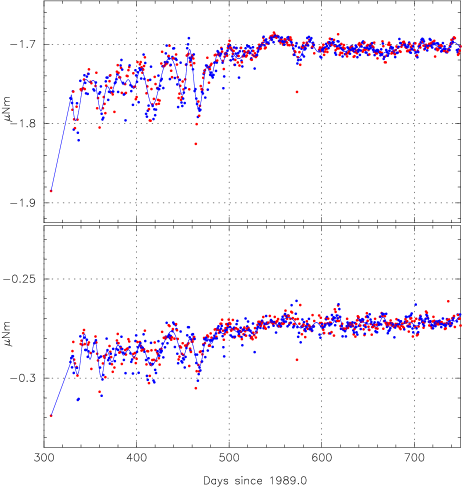
Figure 1: Systematic disturbances in the two main components of the solar-radiation torques around the spin axis after removal of the modulation by the Earth-Sun distance variations. The disturbances around day 400 are also observed in other components of these torques around the spin axis, but not around the other two axes. The disturbances re-occurred after about 570 days, when the same alignment of the Sun, Earth and satellite orbit returned.

The extensive testing of the FDA model in the attitude reconstruction has exposed details on the (non-)rigidity of the spacecraft. Non-rigid behaviour is most clearly shown through scan-phase discontinuities (see the accompanying paper), likely to be the result of discrete, small displacements of one of the solar panels. There are various other subtle indications of non-rigid behaviour. One possible example of non-rigid behaviour is observed from the evolution of the solar radiation torques around the spin axis over the mission (Fig. 1). At times when the satellite passed through perigee such that the normal vector to the solar panels was more or less aligned with the velocity vector of the satellite, and thus perpendicular to the direction of the Earth’s centre (experiencing maximum force from the outer layers of the Earth’s atmosphere), the solar radiation torque components for the spin axis became significantly disturbed. These torque components, which describe the amplitudes of typical harmonics of the rotation period of the satellite, result from shadows of the solar panels on the spacecraft. In order to disturb the amplitudes in a systematic and correlated manner, there are two possibilities: variations in the solar radiation, or variations in the surface of the satellite as seen from the Sun. Solar-flux variations are more than an order of magnitude smaller than the level required by the observed effects, and would also affect the torques on the $x$ and $y$ axes, which is not observed. This leaves only changes in the outer properties of the satellite as an explanation, even though most of these would probably also be observed on the $x$ and $y$ axes. It is still unclear what properties of the satellite could be changed to cause these quite significant and systematic changes.

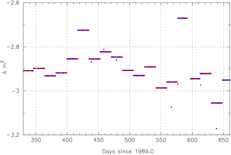
Figure 2: The reconstructed magnetic moment for the $y$-axis. Significant variations took place on at least time scales of a few days. Determinations here cover periods of 40 orbits each (with a few individual determinations still left).

The non-rigidity effects described above are probably causing significant disturbances on the apparent rotations of the satellite, most of which cannot easily be recognised or predicted. The result of this is that the prediction of the torques affecting the satellite can only provide a first approximation of its dynamical behaviour. The detailed behaviour has to be reconstructed for each orbit separately. Further disturbances are probably caused by unresolved small hits. Prediction of torques is also hampered by the presence of magnetic torques, and variations in the satellite’s magnetic moment (Fig. 2) and the magnetic flux in the Earth’s magnetic field. The magnetic moment variations may, occasionally, have been a source of violation of the basic condition of the FDA by causing small discrete variations in the external torques, but for most of the time the underlying torques will still have been continuous. Any magnetic torque variations will be more significant close to perigee (where no observations took place), as around apogee the magnetic field is weak and the resulting torques are quite small.

3.3 Time resolution and weights

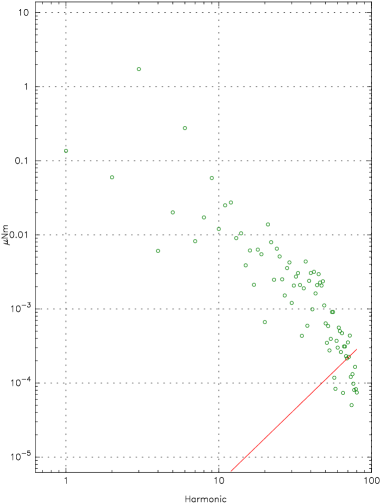
Figure 3: The power spectrum of the spin-synchronous harmonics in the torques acting on the spin axis. The three-fold symmetry of the satellite reflects in the relatively higher amplitudes for the 3^rd, 6^th, 9^th and 12^th harmonics. The line indicates values that would be equivalent to causing a 0.3 mas amplitude in the positional variations.

The time resolution used in the along-scan attitude reconstruction, as well as the density of nodes in the spline fitting, has been determined in first instance from the power spectrum of the harmonic signals in the observed torques (Fig. 3). As a comparison, an amplitude $A_{n}=10^{-4}\mu$Nm for the $n^{\mathrm{th}}$ harmonic in the torques results in an amplitude for the positional variations of $671/n^{2}$ mas. Thus, harmonics up to about $n=70$ are still contributing significant (more than 0.3 mas) positional variations. A full cycle for $n=70$ is equivalent to about 5° on the circle, and 100 s of time, and will require two intervals between nodes to be approximated. Nodes in the along-scan attitude have been placed at nominal distances of about 66 s, and the resolution of single observations at 10.7 s. A single observation combines, as a weighted mean, single-star transit residuals as observed in one field of view. An upper limit is applied to the weight contributions of bright stars to restrict their influence. As a result, the T2 statistics (see for example Papoulis 1991) for these observations are slightly offset (Fig. 4). Any severe outliers are eliminated from calculating the mean.

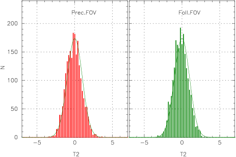
Figure 4: The distribution of T2 statistics for the construction of the mean abscissa residuals per format of 10.7 s. The curves show the ideal Gaussian distribution for the same number of observations. The offsets towards lower T2 values are due to the weight limit applied to the brightest transits.

An important new aspect in the final along-scan attitude reconstruction is the control over the weights of contributions from the two fields of view as applied in the solution. As has been described in the accompanying paper, it is essential for the production of absolute parallaxes and the rigidity of the reconstructed sky to ensure very good connectivity between the fields of view. This can only be achieved if both fields of view are contributing significantly to the reconstruction of the along-scan attitude. In order to obtain a good weight distribution without losing too much information, the weight contributions are assessed for each node interval in the spline function. The weight contributions from the individual observations are added up for each interval, and for each field of view. Whenever the total interval weight of one field of view exceeds that of the other field of view by more than a factor 2.89, the higher weight is reduced to produce the maximum allowed ratio. During the initial tests the weight ratio has been reduced from a starting value of 6 to the current value of 2.89, without noticeable deterioration of the abscissa residuals for the brightest stars. Even at a maximum ratio of 2.89 there are still many iterations needed to obtain reliable absolute parallaxes for all stars in the catalogue. During these iterations minor distortions of the reconstructed sky are slowly smoothed out.

4 Internal statistical tests

A very tight control on the statistical properties of the new reduction has ensured the detection of scan-phase discontinuities, external hits and a few other peculiarities in the data, and has prevented these from penetrating the final astrometric results. The control covers various aspects which can be split in two groups: trend analysis and analysis of residual distributions. In some cases combinations of the two are applied too.

4.1 Trend analysis

Trend analysis is applied to calibration parameters in order to detect outliers that may indicate problems in the reduction. Application to the basic-angle and instrument parameter calibrations, for example, exposes those data sets for which temperature control in the payload was temporarily (partly) lost. Such data sets can either be repaired (allowing additional modelling parameters in the reduction) or rejected.

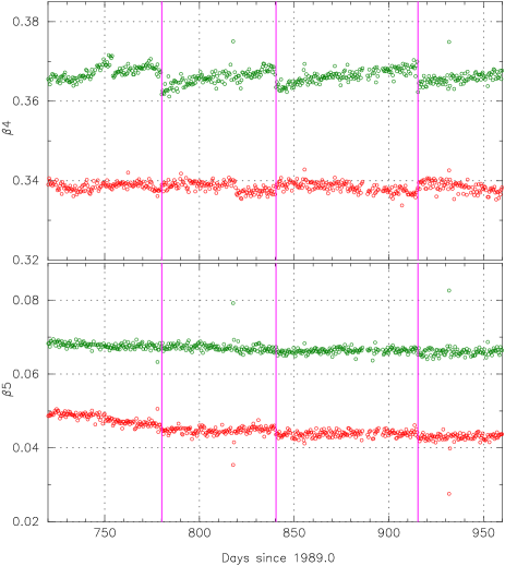
Figure 5: An example of trend analysis, applied here to the calibration of the second-harmonic modulation parameters for the main detector, $\beta_{4}$ and $\beta_{5}$ (see also Section 4.3). Next to the discontinuities caused by re-focusing (vertical lines) disturbances can be seen on day 755 (orbit 1006, change of thermal-control electronics), days 779, 856 and 932 (orbits 1060, 1235 and 1407, re-starting the on-board computer), and day 818 (orbits 1150 & 1151, anomalous voltage). In each graph the upper set of data points refers to the following and the lower set to the preceding field of view.

Trend analysis has been applied to:

• the noise, drift and orientation properties of the gyros;

• the geometric calibration of the star mapper grid;

• the noise properties of the star mapper based attitude solutions;

• the calibration of the optical transfer function for the main detector (describing the relation between the first and second harmonics in the modulated signal as a function of field of view, position on the grid and colour of the star);

• photometric calibration parameters for the main grid;

• instrument parameters and basic angle for the main grid;

• the calibration of scan-rate changes as a function of thruster-firing lengths;

• torque calibration.

In trend analysis the accumulated calibration parameters are displayed as a function of time, with the possibility to focus in or out or pan through the data, displaying the identification of time and orbit number for any position of the cursor in the graph. An example of such a graph is shown in Fig. 5 for the calibration of two modulation parameters of the main detector signal, $\beta_{4}$ and $\beta_{5}$ (see also Section 4.3), which together describe the amplitude ratio and phase difference between the first and second harmonics. It shows the different reaction of the two parameters in the two fields of view to a range of events such as refocusing, changes in thermal control, and a voltage outing. Most of these events also show up in basic angle drifts (see accompanying paper). Thus, trend analysis is used to detect the occasional anomalous conditions for payload operations that may require special attention. By applying it to a wide range of parameters, few, if any, anomalous conditions slip through unnoticed.

4.2 The star mapper based attitude reconstruction

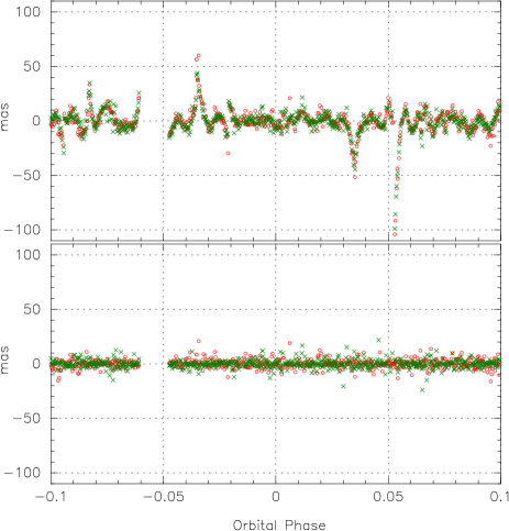
Figure 6: Abscissa residuals for one rotation of the satellite in orbit 401 (early May 1990). The top graph shows the residuals relative to the star mapper based attitude, and displays effectively the performance of that process. The bottom graph shows the same observations after the final iteration in the along-scan attitude fitting. The crosses and circles refer to observations from the preceding and following fields of view. The discontinuities in the upper graph reflect the effect of thruster firings.

The performance of the first step in building the attitude model is illustrated in Fig. 6. In the top graph is shown how the star mapper based attitude (SMA) performs for the reconstruction of the scan phase. With the relatively high noise levels and low density of the star mapper data, the attitude detail that can be fitted using those data is limited. The overall accuracy of the reconstruction is generally within 10 mas, but systematic excursions occur fairly frequently, and can reach up to 200 mas. The main reason for these excursions is generally lack of suitable data. This applies even more so for the reconstruction of the spin axis position: while transits from both fields of view contribute to the along-scan attitude, it is only one field of view that contributes to the reconstruction of one direction of the spin axis.

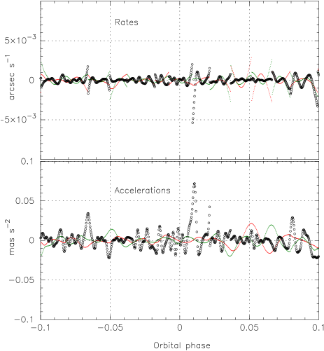
Figure 7: Residuals in rates (top) and accelerations (bottom) for the star mapper based attitude reconstruction. The data cover one rotation of the satellite. The large symbols refer to the along-scan direction, the small symbols to the spin-axis position. Data for orbit 52, 27 November 1989.

The SMA determines more than just the reference pointing model. It also provides information on the inertial rates of the satellite on all three axes. This is required for the reduction of the main grid transits: the rotation rates of the satellite, together with the grid geometry, determine the relation between time and relative modulation phase for the individual samplings of a star transit. The along-scan rate errors as derived from the star mapper data can be as large as $\pm 6$ mas $\mathrm{s}^{-1}$, but are typically within $\pm 1$ mas $\mathrm{s}^{-1}$ (Fig. 7). These errors will only cause a very small amount of additional noise on the amplitudes of the estimated modulation parameters. At 6 mas $\mathrm{s}^{-1}$ the reconstructed amplitudes for the first harmonic is decreased by about 0.004 per cent, and for the second harmonic by about 0.016 per cent. Acceleration errors for the SMA are generally between $\pm 0.06$ mas s^-2 and create errors on the phase estimates below $10^{-3}$ mas. Errors on the SMA are thus unlikely to contribute any significant noise to the estimates of the modulation parameters for the main-grid transits.

4.3 The modulation parameters

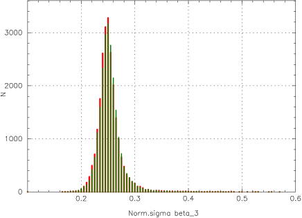
Figure 8: The distribution of formal errors on the modulation phase $\beta_{3}$ in arcsec, multiplied by the square root of the total photon count and the relative modulation amplitude $M1$ for the signal. Data for orbit 75.

The analysis of the modulated signal obtained from transits over the main grid is central to the Hipparcos data analysis. Here we follow the NDAC model, which describes the characteristics of the second harmonic relative to the first harmonic parameters:

$$I_{k}({\bf\beta}) = \beta_{1}+\beta_{2}\bigl{[}\cos(p_{k}+\beta_{3})$$ (4)

$$+ \beta_{4}\cos 2(p_{k}+\beta_{3})+\beta_{5}\sin 2(p_{k}+\beta_{3})\bigr{]},$$

where $p_{k}$ is the assumed modulation phase of the signal $I_{k}$ for sample $k$ as based on the attitude model, which can be the SMA or the result of a previous iteration. The astrometric information is derived from the modulation reference phase, $\beta_{3}$, while $\beta_{4}$ and $\beta_{5}$ together describe the intensity-independent relative amplitude and phase of the second harmonic in the modulated signal. The relations between these parameters and other representations of the modulated signal that lend themselves better for a least-squares solution can be found in Volume 3 of ESA (1997) or van Leeuwen (1997).

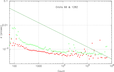
Figure 9: A log-log diagram of the mean formal errors on the predicted positions, as derived from the published catalogue, as a function of the total photon count for frame transits. The data for orbits 66 (open circles) and 1282 (dots) are shown. The formal errors for orbit 66, at the beginning of the mission, are clearly larger (as a result of uncertainties in the reconstructed proper motions) than for orbit 1282, half-way the beginning and end of the mission. The diagonal line shows the average photon-noise relation over the mission for a modulation parameter $M1=0.72$.

The formal error on $\beta_{3}$ is a function of the total photon count received and the relative modulation amplitude $M_{1}\equiv\beta_{2}/\beta_{1}$, which has some dependence on field of view, colour index of the star and position on the grid. The modulation amplitude varies as a function of time as a result of small changes in the optics and has a typical value of 0.72. Over the mission, the error on the modulation phase has been calibrated as:

$$\sigma\beta_{3}\approx\frac{255}{M1\sqrt{I_{\mathrm{tot}}}}\leavevmode\nobreak\ \leavevmode\nobreak\ mas,$$ (5)

where $I_{\mathrm{tot}}$ is the total photon count accumulated for the signal. The factor 255 in Eq. 5 represents an average over the field of view. Over the mission the average amplitude over the field of view decreased slowly, causing this factor to evolve from a value of 249 at the beginning of the mission to 257 for the preceding and 253 for the following field of view. The recovery of this factor is illustrated for one orbit in Fig. 8. Orbits affected by thermal control problems show generally lower modulation amplitudes and thus larger errors on the phase estimates.

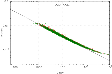
Figure 10: A log-log diagram of the formal errors on the input data for the along-scan attitude reconstruction. Each data point represents 10.7 s of observations in one of the fields of view. The diagonal line is the photon noise relation, and the deviation towards the bright end reflects the formal accuracies of the predicted positions of the stars.

It is further interesting to note that for the transits with the highest photon counts the intrinsic precision obtained over a 2.13 s interval (a so-called frame transit) is already higher than the predicted positional accuracy for the observed star as derived from the published Hipparcos catalogue. This is shown in Fig. 9 for one orbit at the beginning of the mission, and one half-way. The predicted positions naturally have higher errors for the start and end of the mission than half-way due to uncertainties in the reconstructed proper motions.

As was described above, the data for 10.7 s intervals (5 successive frame transits, also referred to as one format) are combined per field of view to provide the input data for the along-scan attitude corrections. The formal errors in the reference positions are fully taken into account when evaluating the formal error for each data point. Each format contains usually more than one observation per star, in which case the formal error for the predicted position is added to the mean of those observations rather than to each observation individually. The resulting errors at the time of the third iteration are shown for one orbit (64) in Fig. 10. The range of formal errors on these data points is about a factor 30, but the error ratio allowed to ensure proper connectivity is only 1.7. Most of the potentially high-precision observations are therefore down weighted in their application to the along-scan attitude solution, depending on the data available in the other field of view. Still, in most cases a formal error of around 2.5 mas is obtained per observation.

4.4 Field transits and abscissa errors

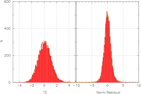
Figure 11: Statistics on field transits. Left: histogram of the T2 statistics for the formation of field transits from frame transits. Right: normalised residuals between field transit abscissae and the predicted positions, for the third iteration. The curves show the equivalent Gaussian distribution for the same number of observations.The data are for orbit 409.

An important feature of the new reduction is the time resolution of the final abscissa data. The Intermediate Astrometric Data in ESA (1997) is in the form of one abscissa for each observed star per orbit of the satellite, incorporating observations from both fields of view. The great-circle reduction process made a higher resolution meaningless. In contrast, the epoch photometry for the mission is presented at field-transit level, which prevents a one-to-one relation between the photometric and astrometric information. In the new reduction the abscissae are preserved at field-transit level. This gives much improved detection possibilities for transit disturbances such as due to the presence of a parasitic image in the other field of view (events that are indicated in the epoch-photometry files). Events like these are characteristic for single field transits only.

Furthermore, creating field transits provides a handle on the internal consistency of the data through the T2 statistics (Papoulis 1991) of the merged frame transits, the basic measurement unit as described above. A typical example of the T2 statistics for the construction of field transits of single stars is shown in Fig. 11. Also shown there is a histogram of the normalised residuals (weighted by the photon-noise errors only) between the field transit abscissae and the predicted catalogue positions (single stars) after the third iteration. Histograms like these are produced for each orbit and form part of the quality control of the data, combining checks on residual distributions with trend analysis.

5 Astrometric parameters

The ultimate check on the internal consistency of the data comes from the abscissa residuals left after fitting the astrometric parameters. This process is iteratively connected with determination and application of differential corrections. Some of these used to be part of the sphere reconstruction, but are now, due to their very small size in the new reductions, solved independently. These corrections are:

• the scan-phase zero point for each orbit,

• small-scale distortions as a function of ordinate over the mission,

• residual chromaticity corrections over the mission.

These corrections are described below, followed by a description of the statistical properties of the abscissa residuals as observed in the astrometric-parameter solutions.

5.1 Final residual corrections

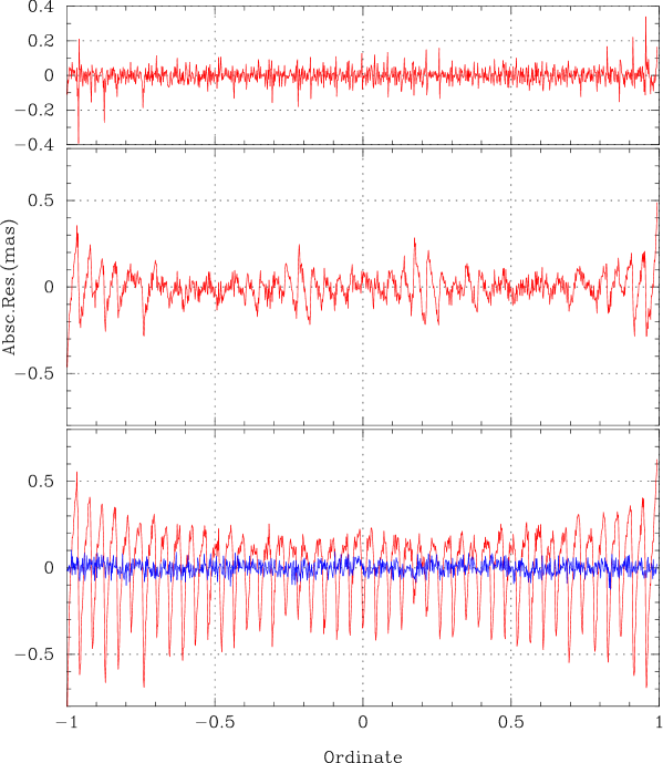
Figure 12: The small-scale distortions as observed across the grid for field transits. Bottom: the actual distortions, showing as a regular pattern the 46 individual rows of scan fields. The large fluctuations represent the mean over the two fields of view, the much smaller fluctuations represent half the difference; Middle: After correcting for a systematic non-linearity of the grid lines; Top: After also correcting for mean scan-field tilt per row.

The scan-phase zero points, which were an important element in the original sphere solutions for the Hipparcos reductions, have almost lost their meaning in the new solution. Sidestepping the great-circle solution effectively removes the scan-phase zero point as a degree of freedom, and what is left is probably little more than the small global distortions of the catalogue. It is therefore no surprise that at the end of the third iteration these residuals are observed to be only of the order of 0.03 mas. Any orbit showing a significantly larger value is checked for data quality.

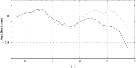
Figure 13: The final chromaticity corrections as derived from the accumulation of abscissa residuals in the astrometric parameters solutions. The full and dashed lines refer to data from the preceding and following fields of view respectively. A linear term (variable over the mission) has already been subtracted as part of the instrument-parameters solution.

There are, however, small-scale distortions affecting the data at a level of up to $\pm 0.6$ mas. These originate from residual colour dependencies of the abscissa residuals (Fig. 13) and from characteristics of the modulating grid, which are summarised here.

The modulating grid of 0.9 by 0.9 degrees consisted of individually printed scan fields, 168 along the scan-direction and 46 perpendicular to it. Each scan field measured about 19.28 by 70.43 arcsec (see Fig. 5 in van Leeuwen 1997, or Fig.2.10 in Volume 2 of ESA 1997). During a frame transit (at nominal scan velocity of 168.75 arcsec $\mathrm{s}^{-1}$) a star would cross about 18 scan fields. There is, therefore, not much resolution in the along-scan direction. In the across-scan direction the resolution is determined by the tilt of the grid (5 arcmin) and the dispersion of the across-scan rotation rate of the satellite ($\approx 1\arcsec$ $\mathrm{s}^{-1}$). The tilt of the grid causes a displacement of 4.7 arcsec across-scan, while the across-scan angular-velocity dispersion is equivalent to about 9 arcsec in positional displacements in a complete field transit.

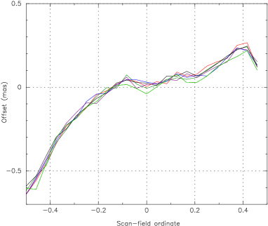
Figure 14: The average distortion of the grid lines across a scan field as measured in frame transits. The seven curves show different intervals (covering each about 380 orbits) over the mission. The scan-field ordinate is normalised to the height of a scan field, 70.43 arcsec.

To show the small-scale distortions as a function of transit ordinate, we accumulated abscissa residuals at a resolution of 24 bins per scan field, equivalent to a bin width of nearly 3 arcsec. The binning therefore does not deteriorate the actual resolution of the signal, which is set mainly by the across-scan angular-velocity dispersion. The bins have been carefully scaled and aligned with the grid pattern, which can very easily be recognised from the accumulated residuals. Systematics up to 0.6 mas are exposed, revealing a general curvature of the grid lines with a peak-to-peak amplitude of around 1 mas, and systematic tilts for rows of scan fields (Fig. 12). In a further refinement, the abscissa residuals have been accumulated at frame-transit level, showing a systematic distortion as well as significant systematics in the tilting of scan fields (Fig. 14). In assessing these values it should be realised that on the physical grid a scan field has a height of just under 0.5 mm, and the distortions shown in Fig. 14 amount to displacements of up to 4 nm, compared to an average grid period of 8.20 $\mathrm{\mu}$m.

The ordinate-dependent distortion cannot be resolved from the published data, as the combination of field-transit data into orbit residuals mixes data with different ordinates. Ordinate information was therefore not preserved in the published data. These distortions form part of the unresolved modelling noise present in the FAST and NDAC results, but played no mayor role given the noise contribution from the attitude modelling in those reductions. With the reduced modelling-noise levels of the new reduction, however, they become significant and are fully incorporated in the instrument model.

5.2 Remaining abscissa dispersions

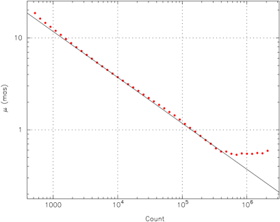
Figure 15: The dispersions in field-transit abscissae as a function of total transit photon count. The diagonal line is the Poisson-noise relation for average signal modulation amplitudes.

The dispersion of the abscissa residuals for field transits has been investigated as a function of the total observed photon count of the field transit and the modulation amplitude $M1$ (Eq. 5). This provides a direct comparison with the statistics observed at earlier stages of the reductions. Such a comparison exposed, at an earlier stage of the reductions, the presence of additional modelling noise, which was ultimately identified as primarily resulting from the scan-phase discontinuities described in the accompanying paper. After identifying some 1500 of these phase jumps, and incorporating that information in the model for the along-scan attitude reconstruction, the dominating noise contributions left are the Poisson and attitude noise, as is illustrated in Fig. 15. The remaining attitude noise at this field-transit level is approximately 0.5 mas, about a factor 5 lower than in the original reductions, where it is at a level of 2 mas at orbit-transit level (there are on average 3.5 to 4 field transits for each orbit transit). The remaining Poisson noise is close to where one could ideally expect it to be.

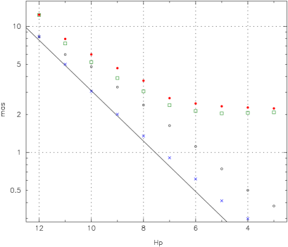
Figure 16: Dispersions in orbit-transit abscissa residuals as a function of magnitude. Squares: NDAC data; Filled circles: FAST data; Open circles: new reduction; Crosses: new reduction normalised in observing time. The diagonal line represents the expected relation for photon-noise statistics.

In order to make a direct comparison with the published data, we combined the field-transit abscissa residuals to create orbit-transit residuals. The statistics of these residuals are compared with those of the published data as a function of magnitude in Fig. 16. This is the equivalent of Fig. 24 in the accompanying paper. The abscissa dispersions as a function of magnitude are affected by differences in observing time. After normalising the dispersions for average amounts of observing time at each magnitude, a nearly perfect Poisson relation is recovered. The abscissa dispersions at orbit level in the new reduction are observed to be lower than the FAST and NDAC results for all magnitudes, but in particular for the brighter stars.

Figure 17: Correlations in the abscissa errors at orbit level for the new reduction. The various measures taken in the new reduction have reduced the abscissa-error correlations by a factor 30 to 40, to a level where they no longer play a significant role. The second set of peaks is at the basic-angle interval of 58°. The data are for stars brighter than 7th magnitude.

A confirmation of the much lower level of attitude noise in the new reductions is obtained from the orbit-abscissa error-correlation statistics. As is explained by van Leeuwen & Evans (1998) and in the accompanying paper, these error correlations form a major obstacle in deriving reliable parallax data for open clusters. Figure 17 shows the situation for the new reduction, and should be compared with a similar plot for the published data such as Fig. 18 in the accompanying paper. In the new reductions these correlations are about a factor 30 to 40 smaller, and no longer have a significant influence on combining data from stars in areas of a few degrees on the sky, thus making derivation of open-cluster parameters much simpler and at the same time more reliable.

5.3 Precision of astrometric parameters

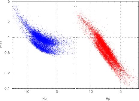
Figure 18: The precisions (formal errors) of parallaxes in the published data (left) and the new solution (right) as a function of magnitude. The bimodal structure in the plots reflects the scanning strategy: around the ecliptic poles the number of observations and their distribution is far more favourable for accurate parallax measurements than around the ecliptic plane.

The precision of the astrometric parameters for stars brighter than about magnitude 7, as presented in the published data, is largely determined by modelling noise rather than photon noise. This modelling noise has been significantly reduced in the present study, and as expected, the same applies to the formal errors on the astrometric parameters for the brighter stars as is illustrated in Fig. 18. The main relation shown for the new reduction in Fig. 18 displays the photon statistics of the data. The scanning strategy reflects in the two bands of formal errors: the lower band is associated with areas within 47 degrees from the ecliptic poles, the upper band with the area within 43 degrees from the ecliptic plane. It is also noted that for the new reduction, unlike the published data, the parallax errors reflect the effects of increased observing time for fainter stars. This can also be observed from the relative increase in noise for the 12^th magnitude stars in the published solution in Fig. 16. It is unclear why in the published data the errors for the faintest stars are larger than could be expected on the basis of their photon statistics. The net result of the new reduction is an improvement in the formal errors over all magnitudes, and most dramatically so for the brighter stars.

6 External statistical tests

As is shown above, the new reduction has a potential parallax accuracy for stars brighter than Hp$=4$ of around 0.1 to 0.2 mas. At these levels of accuracy the tests that have been used before to verify the formal errors on the data have lost their effectiveness: the number of negative parallaxes for stars brighter than $\mathrm{Hp}=6$, for example, is significantly reduced (there is only one marginal example left) and statistically irrelevant. There are also no longer other measurements of comparable accuracy available. However, some information can be gained from the parallax and proper motion data for stars in open clusters. For the Hyades the trigonometric parallaxes can be compared with the dynamic parallaxes. For the Pleiades, Praesepe and a few others the internal consistency of parallaxes and proper motions can be tested. These tests, which become relevant once the iterations through the new reduction have fully converged, will be presented in one or more future papers.

At the current stage of the reductions, the conclusion of the 7th iteration, the parallax adjustments can be recognised in the developments of the differences between the new and old solutions for stars brighter than magnitude 3.5: these differences are still slowly increasing with every next iteration and are at currently nearly representative for the formal errors on the published data. This is a necessary, though not necessarily sufficient, condition for the formal errors on the new reduction results to be reliable.

7 Conclusions

The new reduction of the Hipparcos data as presented here has the potential to significantly improve overall accuracies of the astrometric data obtained with that mission. These improvements stem from changes in the processing technique (the de-coupling of the great-circle reduction processes, the dynamical attitude modelling) and the recognition and accommodation of large numbers of scanning disturbances. Incorporating provisions in the along-scan attitude reconstruction to ensure proper connectivity all over the sky, independent of the local density and brightness of stars, ensures a much improved reliability of the parallaxes. These provisions, however, do require several iterations through the reductions for convergence to be reached.