Rights and wrongs of the Hipparcos data

A critical assessment of the quality of the Hipparcos data, partly supported by a completely new analysis of the raw data, is presented with the aim of clarifying reliability issues that have surfaced since the publication of the Hipparcos catalogue in 1997. A number of defects in the data are identified, such as scan-phase discontinuities and effects of external hits. These defects can be repaired when re-reducing the raw data. Instabilities in the great-circle reduction process are recognised and identified in a number of data sets. These resulted mainly from the difficult observing conditions imposed by the anomalous orbit of the satellite. The stability of the basic angle over the mission is confirmed, but the connectivity between the two fields of view has been less than optimal for some parts of the sky. Both are fundamental conditions for producing absolute parallaxes. Although there is clear room for improvement of the Hipparcos data, the catalogue as published remains generally reliable within the quoted accuracies. Some of the findings presented here are also relevant for the forthcoming Gaia mission.

1 Introduction

1.1 Background

The Hipparcos mission (ESA 1997; Perryman et al. 1997; van Leeuwen 1997; Kovalevsky 1998) involved a wide range of new concepts applied under what accidentally became very difficult conditions. These new concepts were ultimately all aimed at obtaining absolute parallaxes for a selection of approximately 118000 stars and in this the mission largely succeeded. The publication in May 1997 of the catalogue, based on the data reduction results obtained by the two independent reduction consortia FAST (Kovalevsky et al. 1992) and NDAC (Lindegren et al. 1992), took place according to a time schedule set by the Hipparcos Science Team in agreement with the European Space Agency (Perryman et al. 1997). This did not allow for final iterations and reflections on methods used and results obtained to take place. It is therefore not surprising that a number of incidents in the data have not been fully appreciated during the preparation of the catalogue.

Some, but not all, of the problems in the Hipparcos data that have since been detected can be traced back to the orbit anomaly suffered by the mission. Instead of operating at a geostationary position, Hipparcos described a geostationary transfer orbit of 10.7 hours, for which the perigee height had been increased to an average of 450 km (Dalla Torre & van Leeuwen 2003). With a rotation period of just over 2 hours, a single orbit covered close to five revolutions of the satellite. No observations could be made when the satellite was out sight for all of the three ground stations. This always happened for about 2 hours around the perigee passage but could also occur for other reasons. The data obtained during one orbit will be referred to as a data set.

Since the publication of the Hipparcos catalogue, it has appeared that for (small groups of) bright stars one of the two basic conditions for obtaining absolute parallaxes may not always have been properly fulfilled. These two conditions are:

• A very stable basic angle, with variations well below 1 mas over a 10 hour period: all available data show that this condition was well fulfilled for more than 99 per cent of all data sets;

• A reconstruction of the satellite’s scan phase (the so-called along-scan attitude reconstruction) which is at all times based on significant contributions from data obtained in both fields of view. The along-scan attitude reconstruction provides the reference frame for the Hipparcos measurements, which come in the form of transit times or abscissae (the along-scan coordinate of the star (see further Volume 3, ESA 1997)).

The latter condition will be referred to as the “connectivity requirement”. It lies at the heart of the Hipparcos concept: through fulfilling this requirement the effects of parallax displacements in the measurements can ultimately (through iterations with the sphere reconstruction and the astrometric-parameter determinations) be eliminated from the along-scan attitude reconstruction. A reference frame unaffected by parallax displacements is essential for obtaining absolute parallaxes.

A local failure in the connectivity requirement could explain the apparent problem with the Pleiades parallax as derived from the Hipparcos catalogue. That there may be problems with the Hipparcos determination of the Pleiades parallax at 8.35 mas (van Leeuwen 1999a; Robichon et al. 1999) has been suggested by several authors before (Pinsonneault et al. 1998; Soderblom et al. 1998; Reid 1999; Pinsonneault et al. 2000; Stello & Nissen 2001; Pinsonneault et al. 2003), but often without sufficient understanding of how such a discrepancy could occur locally only (Narayanan & Gould 1999). Statistical tests on the data rule out global discrepancies in both the parallax zero point and the formal errors on the astrometric parameters (Arenou et al. 1995; Lindegren 1995). Independent geometric determinations of the Pleiades parallax are very hard to obtain, as the cluster velocity and distance make it unsuitable for a convergent-point determination (van Leeuwen 2005). As not all studies seemed to contradict the Hipparcos result (Castellani et al. 2002; Percival et al. 2003), it remained unclear where the fault may lie. In a more recent paper though, Percival et al. considered the traditional longer distance the more probable (Percival et al. 2005).

Some further information has recently come from studies of individual binary stars in the cluster (Pan et al. 2004; Munari et al. 2004; Zwahlen et al. 2004), which all indicated the larger distance of 130 to 135 pc. The first two of these studies still contain a model element (they are not purely geometric), only the third of these studies provides a pure geometric determination. All three provide the distance of a single star in a cluster with a diameter of 20 pc (van Leeuwen 1980), although as bright stars and binaries they are more likely to be found close to the centre of the cluster (van Leeuwen 1980; Raboud & Mermilliod 1998). The measurements of the parallaxes of a few stars with the HST (Soderblom et al. 2004) also confirm the larger distance, but those observations pertain to differential rather than absolute astrometry.

Limited corrections of the published Hipparcos data are possible and had been foreseen in its preparation by making available intermediate astrometric and photometric data, and providing details of the colour indices used in the data reductions. This made possible, for example, the improvements to the astrometry for the very red, large-amplitude variables (Pourbaix & Jorissen 2000; Pourbaix & Boffin 2003; Knapp et al. 2001, 2003). The repair of potential connectivity problems, however, requires information that can only be obtained from the original, raw data.

The present paper does not intend to settle the question of the Pleiades parallax, but rather to give a frank overview of issues that have surfaced in a new analysis of the raw data as well as in the intermediate data products made available with the Hipparcos catalogue (ESA 1997). As explained above, one of these issues, connectivity, may well have a bearing on the determination of the Pleiades parallax. The present paper is also in a way a justification for the preparation and presentation of a complete new reduction of the raw Hipparcos data, presented in the accompanying paper. To present a complete new reduction of those data involves a very substantial amount of work, which can only be justified if it provides very significant improvements in accuracy and overall reliability. As will be explained in this and the accompanying paper, this is likely to be the case.

1.2 Structure of the present paper

This paper is organised as follows. Section 2 presents issues affecting the reconstruction of the along-scan attitude: methods applied to the reconstruction, and peculiarities of the scanning of the satellite. Although recognised to exist in the original reductions, the frequency and effects of scan-phase discontinuities and external hits had been grossly underestimated, and no measures were available to systematically identify and incorporate these events in the along-scan attitude reconstruction models.

A major role in the original reductions was played by a process referred to as the great-circle reduction (van der Marel 1988; van der Marel & Petersen 1992; ESA 1997; van Leeuwen 1997). This process allowed, through combining the corrections to abscissae, the along-scan attitude and a set of instrument parameters, to obtain a reliable attitude reconstruction even in the presence of relatively high errors on the reference positions for the stars involved. A single great-circle solution used the data obtained over one orbit, and as such involved data for up to four revolutions of the satellite. All data obtained over this interval were projected on a reference great circle to provide a single abscissa measurement for each star observed. These combined abscissae from the great-circle solutions will be referred to as orbit-transits. They combine data for on average 3 to 4 transits through either of the two fields of view. Section 3 presents problems experienced in the great-circle reduction, most of which were indirectly caused by the orbit anomaly. When, due to ground-station unavailability or problems with on-board attitude control, the usable data obtained over an obit covered two revolutions or less, the basic angle between the two fields of view (58°) allowed for instabilities to develop between the estimates of the along-scan attitude and the determination of the abscissa corrections. This could also happen in orbits where the observations were frequently interrupted by Earth occultations (the image of the Earth coming too close to one of the apertures to continue observing).

Section 4 reviews the status of the basic-angle stability. Here we draw mainly from the results of the new reduction to show that the stability of the basic angle has been very good, down to a 0.1 mas level over a 10 hour period. However, 18 orbits (out of 2300) are identified where the basic angle did show a significant drift; in almost all cases these drifts are directly related to known anomalies in the operations of the spacecraft and payload.

Section 5 presents our current understanding of the importance of connectivity: the way data from the two fields of view become connected in the data reductions through the reconstruction of the along-scan attitude. As was stated above, good connectivity and a highly stable basic angle are essential for obtaining absolute parallaxes. We also examine methods suggested for correcting poor connectivity by Makarov (2002, 2003).

In Section 6 some statistical properties of the abscissa data in the published catalogue and the role played by the merging of the data from the two reduction consortia are reflected upon. The verification possibilities of the formal errors and the parallax zero point for the published data are also briefly reviewed in Section 7. Finally, Section 8 summarises the conclusions of the current study.

1.3 Presentation

Formal errors on abscissa measurements presented here are generally examined as a function of the total photon count or integrated intensity of the underlying observations. The observing strategy for Hipparcos led to variable amounts of integration time being assigned to observations, depending on stellar brightness as well as on the presence of other program stars on the main detector area. The integrated intensity is therefore a much more representative quantity for accuracies than is the stellar magnitude.

Data sets will generally be referred to by their orbit number. Orbits were numbered sequentially as they took place, irrespective of whether data was collected. The first orbit formed part of the test phase and took place on 5 November 1989, while the actual survey began at orbit 48 on 26 November 1989. The last orbit with data, orbit 2769, took place 1207.8 days later, on 18 April 1993.

The abbreviation “mas” will be used for 10^-3 seconds of arc. Torques will often be represented in the equivalent units for acceleration (mas s^-2) rather than in Nm, with values directly related through the diagonal elements in the inertia tensor. In integrations for the dynamical modelling, however, all calculations are done using the full inertia tensor and torques expressed in the proper units.

1.4 Other information

It is in no way the intention of the current study to discredit the work and products of the two data reduction consortia. Much more powerful computing hardware makes investigations possible that were quite difficult 10 to 15 years ago. Processing power, data handling facilities and graphical display capabilities have all improved very significantly over those years.

This study has progressed over 7 years, starting from the basic ideas of the FAST and NDAC consortia on the reduction of the data, and some elementary parts of the new reduction are still identical to what was developed 20 years ago. It shouldn’t harm anyone to have a critical look at what was done then, to see if better results may be obtained from the same data. The Hipparcos data can never be replaced, and if more accurate and reliable information can be extracted from it, then this has to be done, and can only be done by studying in great detail the raw data and intermediate results from the published data. The stars most likely to be significantly affected by any potential improvements of the Hipparcos astrometric data are the brightest stars (V$<8$), for which the main contributions to the formal errors on the astrometric results in the published catalogue are modelling errors rather than photon noise. New missions, like Gaia, will find it difficult or impossible to obtain data for these stars, for which the images may be fully saturated.

2 Scanning problems

Problems related to scanning naturally split in two components: the characteristics of the actual scanning motion of the satellite, and our modelling of these characteristics. The second part of the problem is generally referred to as the attitude reconstruction. In the Hipparcos reductions little attention was given to the first part: it was generally considered too complex for modelling, and exact cubic splines were used to fit positional displacements for the attitude modelling, irrespective of the dynamics of the satellite. The only exceptions are the preliminary studies on the torques affecting the satellite by van Leeuwen et al. (1992) and van Leeuwen (1997) as part of the NDAC activities. In the following sub-sections a brief summary of steps taken in the attitude reconstruction is presented, followed by descriptions of the three main disturbances observed in the scanning motion of the satellite: the scan-phase discontinuities, the external hits and the torque irregularities. A more detailed discussion of the methods used in the attitude reconstruction can be found in Volume 3 of ESA (1997) and van Leeuwen (1997).

2.1 Steps in the along-scan attitude reconstruction

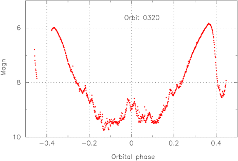
Figure 1: The background in the V channel of the star mapper for orbit 320 (end March 1990). The vertical scale is given as an approximate equivalent of stellar magnitude. The horizontal scale goes from perigee at -0.5 to apogee at 0.0 to perigee at 0.5. One full orbit covers close to 5 revolutions of the satellite. Visible near the centre of the graph are the crossings of the two fields of view through the zodiacal light and the galactic plane. These crossings are repeated around phases -0.2 and +0.2.

The Hipparcos attitude reconstruction consisted of two main steps: a first approximation for all three coordinates using the star mapper data (Donati & Sechi 1992; van Leeuwen et al. 1992), followed by an improvement in the along-scan attitude based on the main detector measurements as part of the great-circle reduction (van der Marel 1988; van der Marel & Petersen 1992). The first stage of the attitude reconstruction had two purposes: to provide the instantaneous position of the spin axis of the satellite to a $1\sigma$ accuracy of 100 mas, and the along-scan attitude with a similar or better accuracy. The first was set by the great-circle solution (see Section 3) and was based on the noise introduced when projecting transits on a reference great circle. The second requirement was essential for the proper identification of a star position on the modulating grid during a transit. The modulating grid had a period, as projected on the sky, of 1.2074 arcsec, and excessively large errors in the first step of the attitude reconstruction could lead to slit ambiguities.

The first stage of the attitude reconstruction, using the star mapper data, could at times be badly affected by high detector noise, in particular during transits of the Van Allen Belts, which took place twice every orbit (Fig. 1). The background signal during these transits often left all but the brightest stars obscured, thereby limiting severely the possibility to accurately reconstruct the attitude. Away from those regions, the $1\sigma$ errors on the reconstructed position of the spin axis were around 80 mas, and for the along-scan phase estimates around $\approx 40$ mas, but it is likely that for periods of high background the errors were considerably larger.

In the second step of the attitude reconstruction the differences between the predicted and observed positions for the main-grid transits were fitted using cubic splines, while at the same time estimating the corrections to the predicted positions. It is from graphs of these differences that scan-phase discontinuities and external hits can be recognised.

2.2 Scan-phase discontinuities

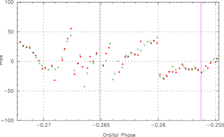
Figure 2: Scan-phase discontinuities are observed when the satellite is warming up or cooling down rapidly, for example after an eclipse as shown here for orbit 253 (Febr.1990). The discontinuities reflect discrete adjustments of the structure of the satellite to the changes in temperature. Here 4 jumps (at phases -0.2676, -0.2667, -0.2640, -0.2600) of around 40 to 70 mas in scan phase are observed from the abscissa residuals with respect to the star-mapper based reconstruction of the along-scan attitude. The crosses and circles represent data from the two fields of view. The data points are weighted averages over 10.6 s of observations. The vertical lines represent thruster firings.

Scan-phase discontinuities are briefly explained in Volume 2 (Section 11.4) of ESA (1997), where their effect on the data was considered insignificant, as at that stage only very few had been detected. In the new reduction of the data, however, some 1500 discontinuities ranging from 20 to 120 mas have been identified as the main source behind a non-Gaussian noise component in the abscissa residuals.

A scan-phase discontinuity is like a jump (Fig. 2), and as such is directly related to the rigidity of the satellite: as the total angular momentum of the satellite is not affected, a jump has to be the result of one part of the satellite moving with respect to some other part. A clear indication of which part may be moving comes from the temporal distribution at which jumps take place: a large fraction is directly linked to eclipses, when the satellite moves in to, or out of, the Earth shadow. These jumps appear to be immediate reactions to the strong temperature changes taking place at these instances (Fig. 3). Jumps are otherwise found to be concentrated around (but not restricted to) an interval of about $45\degr\pm 25\degr$ in the rotation phase of the satellite. The rotation phase, by definition, represents the direction of the solar radiation seen from the satellite. Both aspects point to an external element of the satellite, and the most obvious candidate is any one of the three solar panels, as was also identified in the earlier preliminary investigations on this subject.

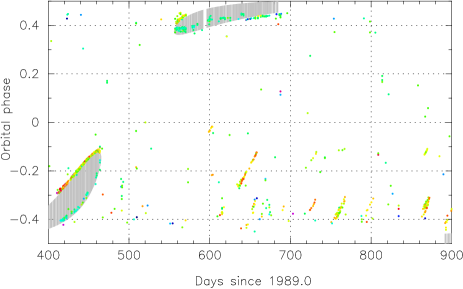
Figure 3: The distribution of scan-phase discontinuities over 500 days of the mission. Every dot represents a recorded jump. The grey areas are times of eclipses. Jumps are clearly concentrated towards the start and end of eclipses, but also occur systematically away from those events. As the orbital period of the satellite was close to five complete rotations, the rotation phase of the satellite for a given orbital phase changed little from one orbit to the next. Jumps tend to concentrate around a fixed rotation phase of the satellite, causing the high levels of correlation in the diagram.

We can estimate the amplitudes of the possible displacements from the sizes, masses and inertia moments involved. Each solar panel measures 1.69 by 1.39 m and has a mass of 6.363 kg. They are connected (on the shorter side) to the spacecraft at 0.9546 m from the spin axis. Assuming an even mass distribution, the inertia moment of a single solar panel around the spin axis is $23.15\leavevmode\nobreak\ \mathrm{kg\leavevmode\nobreak\ m^{2}}$. The inertia moment around the spin axis for the entire satellite is $459\leavevmode\nobreak\ \mathrm{kg\leavevmode\nobreak\ m^{2}}$, giving a ratio of $1:19$ for a single solar panel versus the rest of the spacecraft. The rotational displacement of a solar panel required to give a 40 mas rotation of the payload is therefore just over 0.75 arcsec. At the point of attachment of the solar panels, a 0.75 arcsec rotation amounts to a shift of 3.4 $\mu$m. Thus, very small discrete displacements in the solar panel positions with respect to the spacecraft are sufficient to cause the observed scan-phase discontinuities.

Jumps tend to be negative at the start of an eclipse, and positive after, which may be expected when heating up and cooling down cause opposite movements. Jumps do occur also in a systematic manner away from eclipses, and are noticeably more frequent in the few hours after the perigee passage (Fig. 3). During the perigee passage the outer layers of the Earth atmosphere can affect the temperature of the solar panels, and possibly in some cases even the position.

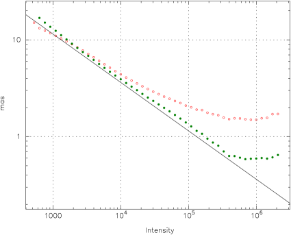
Figure 4: The reduction in the abscissa dispersions due to, amongst others, the detection of scan-phase jumps shows in a comparison between results before removal (open symbols) and at the end of the fourth iteration (filled symbols), when nearly all these defects had been detected and incorporated in the modelling. A further difference is visible for the low intensities, where in the earlier stages of the reduction the cut-off criterion for poor-quality measurements had been set too low, creating artificially low dispersions. The slope of the diagonal line represents the contribution of the Poisson-noise.

The overall effect of phase jumps on the published data is difficult to assess. The amount of data potentially directly affected can be estimated from the number of jumps detected: around 1500. The time interval around a jump for which the attitude reconstruction is affected if the presence of the jump is not incorporated in the attitude model is about 150 s. The total amounts to approximately 3 to 4 per cent of the mission. It is difficult to estimate how these jumps may have affected the along-scan attitude reconstruction in the great-circle reduction due to the way the data are projected on a reference great circle. As a result, local problems in the scanning can replicate between different revolutions of the satellite and between different parts of the scan. The affected time may therefore be much larger, with the effects of a phase jump repeating at intervals of the basic angle, 58°. Such error correlations are observed in the statistics for abscissa residuals (van Leeuwen & Evans 1998) for intervals up to eight times the basic angle. This “spreading out” of scan-phase problems is for example displayed by the systematic effects observed in the abscissa residuals in orbits 721 to 796 (covering days 638 to 660 in Fig. 3). These orbits are all affected by phase jumps that are not directly associated with an eclipse. The abscissa residuals for these orbits in both the FAST and NDAC solutions show a relatively high level of systematics, spread over all rotation phases, and in some cases resembling phase jumps. Contrary to the assumptions for the published data, statistics from the new reduction clearly indicate that these phase jumps did impose a significant, non-Gaussian, noise component on the abscissa residuals. This is shown most clearly in the noise levels of the abscissa residuals before and after detecting and taking care of these events (Fig. 4).

2.3 External hits

The first hits of the spacecraft were recognised by the NDAC team during initial inspections of the gyro data. A hit of the spacecraft causes a discontinuity in its inertial rates. Such discontinuities were also caused by thruster firings, but the instances of the firings were known from the satellite telemetry, and firings always took place in a designated time interval. Inertial rate discontinuities not associated with thruster firings and not in the designated time interval could safely be attributed to external hits. The largest of these caused rate changes at a level of a few arcsec $\mathrm{s}^{-1}$ and four of these have been recorded over the mission. In the NDAC solution these events were incorporated in the attitude model in the same way as thruster firings; in the FAST reductions the gyro data were not analysed and the affected data have most likely been rejected at some stage in the reductions.

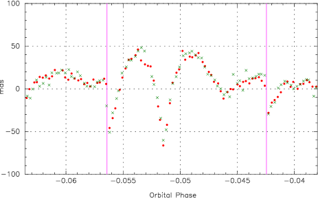
Figure 5: A small external hit of the satellite as reflected in the abscissa residuals relative to the star-mapper based scan-phase reconstruction. The data are for orbit 715 (Oct.1990), for which the scan velocity at orbital phase -0.05148 changed abruptly by 4.7 mas $\mathrm{s}^{-1}$. The crosses and circles represent data from the two fields of view. The data points are weighted averages over 10.6 s of observations. The vertical lines represent thruster firings.

Many more smaller hits took place, but these could not be recognised from the gyro data because of noise levels. Smaller hits do show up, however, in the behaviour of the abscissa residuals with respect to the star-mapper based attitude reconstruction, as shown by the example in Fig. 5. Some 150 of these hits have now been recorded, none of which had been incorporated in the reduction of the Hipparcos data. As with the phase jumps, the fraction of time directly affected is relatively small, about 0.4 per cent, but due to propagation in the great-circle reduction, more data may have been indirectly affected.

The actual energy transfer associated with a hit producing a $\Delta\omega=5$ mas $\mathrm{s}^{-1}$ rate jump is surprisingly small. With an inertia moment around the spin axis of $\mathrm{\textbf{I}}_{zz}=459\leavevmode\nobreak\ \mathrm{kg\leavevmode\nobreak\ m^{2}}$ and a nominal scan velocity of 168.75 arcsec $\mathrm{s}^{-1}$, the change in rotational energy is about 9nJ. The change in angular momentum provides a lower limit of the typical particle mass involved:

$$m\leq\frac{\Delta\omega\mathrm{\textbf{I}}_{zz}}{v\cdot r_{\mathrm{max}}},$$ (1)

where $v$ the velocity of the particle, and $r_{\mathrm{max}}$ the maximum arm-length of the impact position (about 0.95 m). At typical velocities of around 30 km $\mathrm{s}^{-1}$, the masses of the particles involved are small ($10^{-3}$ to $10^{-4}$ mg). However, the shape of the satellite is such that the torque for the spin direction caused by a particle hit will have been relatively inefficient in most cases, and the actual particle masses involved in these hits are likely to be larger than indicated by the angular-momentum transfer for the spin axis. The same uncertainty of where a particle may have hit, and how much it changed the rates on the other two axes (where due to the 100 times higher noise levels the measurements are too unreliable), means that we cannot obtain reliable statistical information from these events.

2.4 Torque disturbances

Figure 6: Reconstructed torques around the spin axis for one rotation of the satellite around apogee, expressed in equivalent accelerations. From top to bottom: orbits 1317, 1318 and 1320. The torques in orbit 1318 are significantly disturbed, possibly due to solar wind following high solar activity.

Torque disturbances are observed around apogee during or shortly after times of high solar activity (Fig. 6). These may be related to the position of the bow-shock of the Earth’s magnetic field, which can go down to the altitude of geostationary orbits in the presence of strong solar winds. The main effect on the data is a requirement for a significant increase in the number of nodes in the spline function, which can weaken the solution. In the NDAC and FAST data analysis increases in the number of nodes were determined automatically on the basis of the dispersion of the data. In the published data, the data sets concerned do not appear to be badly affected.

Problematic attitude behaviour was also encountered around the start and end times of eclipses, when solar radiation torques change rapidly. It is difficult to retrace in the Hipparcos data how the NDAC and FAST solutions coped with these situations, as the same orbits are also affected by the scan-phase discontinuities. In both reduction chains the abscissa residuals for these orbits show well above average levels of abscissa-error correlations.

2.5 Conclusions on scanning problems

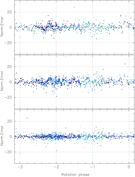
Figure 7: Abscissa residuals for part of orbit 237. From top to bottom: results from the FAST, NDAC, and new reductions. The residuals in the FAST and NDAC solutions are clearly correlated, which may be a reflection of the presence of uncorrected scan phase discontinuities in this orbit.

A re-analysis shows that scanning problems affect the quality of the Hipparcos data for a significant number of orbits. The great-circle reduction procedure tended to transpose any such problems to other parts of the great-circle solution due to the simultaneous solution for the abscissa corrections and the along-scan attitude modelling (see Section 3).

One aspect of the systematics in the abscissa residuals is the way these are often correlated between the FAST and NDAC solutions, as shown for example in Fig. 7. These correlations had also been noticed by Frédéric Arenou (see Volume 3, Chapter 17, of ESA 1997). They could be expected in two situations: when there are (common) systematic errors in the astrometric catalogues used for the final reductions, or when the errors are caused by intrinsic, uncorrected problems with the data, such as scan-phase or velocity jumps. The first solution seems unlikely (but can’t be entirely excluded) due to the independent developments of intermediate catalogues used in the reductions. The second solution is more plausible, and could be the result of the scanning problems (scan-phase discontinuities, hits) described above. In both cases there is clear room for improvements in the Hipparcos results.

3 The great-circle reduction

3.1 Brief overview

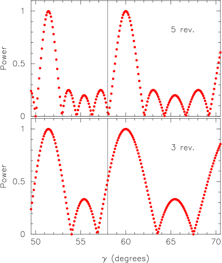
Figure 8: Resonance tests (see text) on basic angle values for 5 (top) and 3 (bottom) revolutions of the satellite. The value of 58° at 5 revolutions was chosen, but this allowed some resonances in the recovery mission, where the lengths of data sets are rarely more than 4 revolutions.

For an overview of the mechanism of the great-circle reduction the reader is referred to van Leeuwen (1997) or Volume 3 of ESA (1997). Here only the main points will be reviewed.

The great-circle reduction (GCR) combined the solutions of three parameter sets: corrections to the along-scan attitude, the stellar abscissae, and the instrument parameters. These solutions were linked to accommodate the rather large errors in the a priori astrometric data for the mission’s program stars. By measuring the same stars several times over one orbit the contributions from the three parameter sets could be disentangled. For the nominal mission the length of time covered by one great-circle solution would have been 5 revolutions (of 2.13 h) of the satellite, resulting in on average 6 to 7 field transits per star. The basic angle had been optimised at 58° for this situation. Optimisation is obtained through convolving observations of the two fields of view in successive revolutions of the satellite with a sinusoidal function with a period equal to the basic angle. This is done for different numbers of satellite revolutions and different basic angles, as shown in Fig. 8 for 3 and 5 revolutions: when an integer number of basic angles fits within an integer number of revolutions of the satellite, a resonance is created which can lead to instabilities in the astrometric solution.

The limitations imposed by the recovery mission provided between 2 and 4 revolutions, and an average over the mission of 3.5 field transits per star per orbit. To see how this may have affected the overall quality of the Hipparcos data, the abscissa residuals as provided for each star in the Intermediate Astrometric data file of the Hipparcos catalogue were regrouped again per orbit and reduction consortium.

3.2 Short data sets

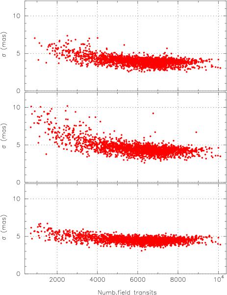
Figure 9: The abscissa dispersions for stars brighter than 8^th magnitude against the total number of field transits (as a measure of the time coverage of the data). Each point represents the data for one orbit. From top to bottom: results for FAST, NDAC and the new reduction. Increased dispersions for the short data sets (low numbers of field transits) are an indication of the instabilities that could occur in the great-circle solution. The application of a $3\sigma$ cut-off for outliers make the FAST and NDAC data look better than the new reduction, where no cut-off is applied other than as indicated by signal-quality criteria.

An indicator of the global quality of the great-circle reduction results is the abscissa dispersion for the brighter stars. Figure 9 shows the results for the FAST, NDAC and new solutions, with a clear increase in dispersion for the shortest data sets, but also with the majority of the data sets performing quite well. In the weighting of the abscissa residuals for the astrometric parameter solutions of individual stars, the formal errors took into account the overall variance of the abscissae in an orbit. Whenever the variance was above average, however, the abscissa errors were mostly systematic rather than random. An example of this is shown in the results for orbit 95, December 1989, containing two large gaps due to Earth occultations which prevented the ring in the great-circle reduction from being closed (Fig. 10). The closing of the ring, achieved by obtaining data well distributed over a great circle, was an essential condition to stabilise the solution. The way these systematic errors have been dealt with in the further application of those data is clear when examining the formal errors assigned to the abscissa residuals, and comparing these with a well-covered orbit (Fig. 11, where the total transit intensities have been reconstructed from the new reduction). The effect of this on the final astrometric data is probably small. For the majority of brighter stars the formal errors assigned to the abscissa residuals in data sets with large systematic errors are relatively large so that they added little weight to the solutions. The new solution allows a full recovery of all data thus affected.

Figure 10: The abscissa residuals for orbit 95 in the three reductions, showing the systematics left by instabilities in the great-circle reduction as applied by FAST and NDAC.

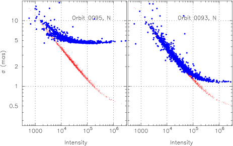
Figure 11: Formal errors of abscissa residual as a function of total intensity of the transit for orbits 95 (see also Fig. 10) and 93 in the NDAC reduction. The thin dots in the background are the equivalent values for the new reduction, for which the formal errors are given as a function of the total transit photon count or integrated intensity and the relative modulation amplitude (see Section 5.1). The systematic errors in orbit 95 were hidden behind large formal errors assigned to the abscissa residuals.

3.3 The 6^th and 12^th harmonics

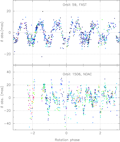
Figure 12: Top: The abscissa residuals for orbit 59 in the FAST reduction, the only orbit left with a clear 6^th harmonic modulation of the abscissa residuals. Bottom: the same for orbit 1506 in the NDAC reductions, an extreme example of a 12^th harmonic modulation.

The so-called $6^{\mathrm{th}}$ harmonic concerned a special kind of instability in the great-circle reduction caused by the proximity of 6 times the basic angle to a full circle. As shown in Fig. 8, this significantly reduced the stability of shorter data sets. The $6^{\mathrm{th}}$ harmonic has been removed from the data as part of the sphere solution, though one data set in the FAST reductions seems to have slipped through (orbit 59) and constitutes an example of how data sets could be affected (Fig. 12). No other FAST or NDAC data sets appear to be affected. However, 12^th harmonics were left in the data, and an extreme example of this is also shown in Fig. 12. The occurrence of strong 12^th harmonics in the abscissa residuals is generally restricted to data sets with less than one full revolution. Most of these data sets have only been accepted by NDAC, but data sets with quite significant 12^th harmonics do also occur in the FAST reductions.

3.4 Conclusions on the great-circle reduction induced effects

The coupling of the three parameter solutions in the great-circle reductions was necessary at the start of the processing because of the relatively high errors in the initial astrometric parameters for the program stars. The special conditions of the mission added vulnerability to instabilities to this process, but the vast majority of data sets are largely unaffected. Using the astrometric parameters as published in a new reduction shows that the solutions of the three parameter sets can now be de-coupled, eliminating these instabilities.

4 The basic angle

The stability of the basic angle, the angle between the two fields of view, constitutes a critical requirement of the Hipparcos mission concept. It is one of the two fundamental conditions for obtaining a rigid reconstruction of the sky and determines a limit on the final accuracies of the astrometric parameters. One specific systematic modulation of the basic angle changes the zero point of the parallaxes and needs to be avoided above all others.

4.1 Relation with the parallax zero point

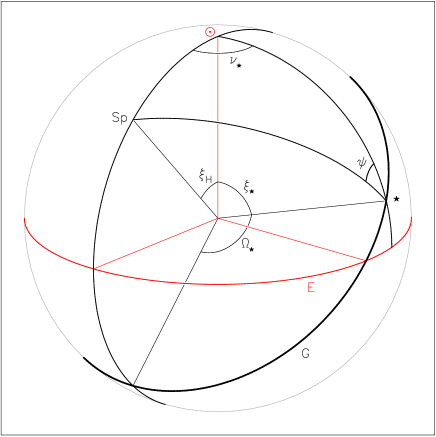
Figure 13: A great circle (G) in the heliotropic reference frame, showing the relation between the angles $\psi$, $\Omega_{*}$ and $\xi_{\mathrm{H}}$ for the calculation of the parallax displacements along the circle for a star (*). The direction of the spin axis is indicated by “Sp”.

To investigate the relation between a parallax zero-point and a modulation of the basic angle we first look at parallax displacements in a heliotropic reference frame: a reference frame in which the direction of the Sun is fixed (Fig. 13). We assign the North-pole of this reference system to the direction of the Sun. The displacement resulting from a parallax $\varpi$ is now restricted to the meridian, and a function of the co-latitude $\xi$ only:

$$\Delta\xi(t)=\varpi\sin\xi(t),$$ (2)

which reaches, as expected, a maximum for $\xi(t)=90$°. The time dependence reflects the inertial rotation of the heliotropic reference system. Almost every great circle in the Hipparcos survey is tilted by 43° with respect to this system, the only exceptions are the Sun-pointing data sets, which are tilted by 0°. In the coordinates of Fig. 13 the local inclination of the great circle with respect to the local meridian is given by the angle $\psi$:

$$\sin\psi=\frac{\sin\Omega_{*}\sin\xi_{\mathrm{H}}}{\sin\xi_{*}},$$ (3)

where $\xi_{*}$ is the contemporary value of $\xi(t)$ for the star observed, and $\Omega_{*}$ the orientation phase or abscissa of the star. Thus, for Sun-pointing data sets ($\xi_{\mathrm{H}}=0\degr$) all parallax displacements along the circle are zero. In all other cases, the parallax displacements along the great circle are given by:

$${\rm d}a=-\Delta\xi\sin\psi,$$ (4)

which, together with Eq. 2 gives:

$${\rm d}a=-\varpi\sin\Omega_{*}\sin\xi_{H}.$$ (5)

Thus, the parallax displacement along the great circle only depends on the abscissa of the star and the instantaneous solar aspect angle of the satellite’s spin axis ($\xi_{\mathrm{H}}$), but not on the ordinate $\xi_{*}$ of the star. What is important here is the coefficient $\sin\Omega_{*}$ in the parallax-offset relation. If a similar coefficient can be caused by modulation of the basic angle, then the zero-point of the parallax system is no longer secure.

To understand the mechanism of the derivation below it is important to realise how the two processes which, through iterations, ultimately determine the Hipparcos catalogue, operate. The first, the along-scan attitude reconstruction, uses abscissa residuals as observed for stellar transits in the two fields of view at the same instance of time (or rotation phase $\Omega_{H}$ of the satellite). The only distinction between the data from the two fields of view is through a fixed correction (per orbit) to the assumed value of the basic angle. The second process, the astrometric parameter determination, uses data for the same star as observed in the two fields of view at different times. All observations of a star during one orbit are associated with a nearly fixed value of the orientation angle $\Omega_{*}$. Every $\Omega_{*}$ value differs from two associated $\Omega_{H}$ values by $\pm\gamma/2$, and vice versa ($\gamma$ is the basic angle between the two fields of view, $\gamma/2\approx 29$ degrees). This determination makes no distinction between data from the two fields of view.

We will examine the effects of a modulation of the basic angle by $\delta h_{0}=A\cdot\cos\Omega_{\mathrm{H}}$, where $h_{0}$ is defined as the correction to half the basic angle and the subscript “H” refers to the position of the satellite $x$-axis. This modulation reflects in the abscissa residuals differently for observations of the same star in the preceding or following field of view:

$$\mathrm{d}a_{\mathrm{p,*}} =\phantom{-}A\cdot\cos\Omega_{H,p} =\phantom{-}A\cdot\cos(\Omega_{*}-\gamma/2),$$

$$\mathrm{d}a_{\mathrm{f,*}} =-A\cdot\cos\Omega_{H,f} =-A\cdot\cos(\Omega_{*}+\gamma/2).$$ (6)

For the astrometric-parameter determination, the average combined effect from the two fields of view is:

$$\mathrm{d}a_{*}=A\cdot\sin\Omega_{*}\sin(\gamma/2),$$ (7)

which is directly correlated with the parallax displacements as given by Eq. 5. Such a modulation of the basic angle will produce a systematic offset in the measured parallaxes: on average, the parallax measurements for all stars will be offset by a fixed amount of:

$$\varpi_{0}\approx-A\frac{\sin(\gamma/2)}{\sin\xi_{\mathrm{H}}}.$$ (8)

A parallax zero-point offset will affect the along-scan attitude reconstruction, which in turn affects the measured abscissa residuals. In order to estimate a possible equilibrium that may be reached for these corrections, an additional “efficiency” factor $F$ is included in Eq. 7:

$$\mathrm{d}a_{*}=A\cdot\sin\Omega_{*}\cdot\sin(\gamma/2)\cdot F,$$ (9)

The parallax zero-point offset is similarly affected by this factor:

$$\varpi_{0}\approx-A\frac{\sin(\gamma/2)}{\sin\xi_{\mathrm{H}}}\cdot F.$$ (10)

The abscissa offsets as a result of the parallax zero point for a given value of $\Omega_{H}$ are (Eq. 5):

$$\mathrm{d}a_{p,H} = -\varpi_{0}\sin(\Omega_{H}+\gamma/2)\sin\xi_{H},$$

$$\mathrm{d}a_{f,H} = -\varpi_{0}\sin(\Omega_{H}-\gamma/2)\sin\xi_{H}.$$ (11)

The attitude model uses the average of the abscissa residuals for the two fields of view:

$$\mathrm{d}a_{H}=-\varpi_{0}\sin\Omega_{H}\cos(\gamma/2)\sin\xi_{H},$$ (12)

which together with Eq. 10 gives:

$$\mathrm{d}a_{H}=A\sin\Omega_{H}\sin(\gamma/2)\cos(\gamma/2)\cdot F,$$ (13)

which is the attitude modulation caused by the parallax zero point, and relative to which the abscissa residuals are measured. For a given star, there will be contributions of this kind from observations in the preceding and following fields of view:

$$\mathrm{d}a_{p,*} = A\sin(\Omega_{*}-\gamma/2)\sin(\gamma/2)\cos(\gamma/2)\cdot F,$$

$$\mathrm{d}a_{f,*} = A\sin(\Omega_{*}+\gamma/2)\sin(\gamma/2)\cos(\gamma/2)\cdot F.$$ (14)

The average of these contributions equals:

$$\mathrm{d}a_{*}=A\sin\Omega_{*}\sin(\gamma/2)(\cos(\gamma/2))^{2}\cdot F.$$ (15)

Equilibrium can be reached in the iterations when the actual abscissa offsets caused by the basic-angle modulation as given by Eq. 7 equal the sum of the contributions from the induced attitude modulation (Eq. 15) and the measured abscissa residuals (Eq. 9):

$$1=(1+(\cos(\gamma/2))^{2})\cdot F,$$ (16)

where we divided left and right by the common factor $A\sin\Omega_{*}\sin(\gamma/2)$. Thus, $F=(1+(\cos\gamma/2)^{2})^{-1}$, and the parallax zero point becomes:

$$\varpi_{0}=-A\frac{\sin(\gamma/2)}{(1+(\cos(\gamma/2))^{2})\sin\xi_{H}}\approx-0.40A.$$ (17)

Extensive tests of the zero point of the Hipparcos parallaxes have revealed no systematic offset down to an accuracy of 0.1 mas (Arenou et al. 1995; Lindegren 1995), from which we can infer $|A|<0.25$ mas. The equivalent factor for the Gaia design is 0.70 (assuming $\gamma=99.4\degr$ and $\xi_{H}=50\degr$), making Gaia more sensitive to such disturbances than Hipparcos was.

Any other systematic spin-synchronous modulation will be uncorrelated with the parallax displacements and will be absorbed in the attitude modelling and abscissae noise.

4.2 Basic-angle evolution, stability and drifts

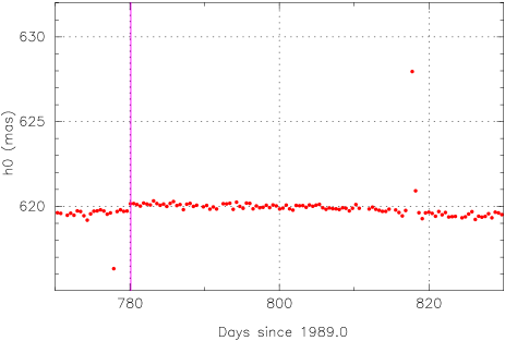
Figure 14: Basic-angle calibration values over a period of two months. For the general trend the basic-angle variations are well below 1 mas, but at two instances deviating values are observed. Both are directly related to known payload anomalies (new reduction). The vertical line at day 780 represents a refocusing of the instrument.

Calibration of the basic angle was performed whenever sufficient data was available. In general the basic angle shows only a slow evolution with time, but on a number of occasions significantly deviating values are observed. Both phenomena can be seen in Fig. 14, where outlying points are observed for orbit 1060 (day 778) and orbits 1150 and 1151, day 818. The first of these is an example of the most common reason for discrepant results: a restart of the on-board computer. These restarts were necessitated by telemetry problems, and caused the entire payload, including heater control, to be switched off. By the time control was restored, the payload had changed temperature, which reflected in a change of the basic angle. Usually, within a few hours the temperature and basic angle value were back at their nominal values. Another example of this kind of event is shown in Fig. 15 for orbit 852 (day 686). A general characteristic of orbits thus affected is that a large fraction of the orbit, usually two rotations of the satellite or four hours, was spent on the recovery procedure, and did not produce observations. The second event visible in Fig. 14 is due to a one-off anomaly, which was referred to in the operations report as an “anomalous under voltage”.

Drifts of the basic angle correction $h_{0}$ of up to 20 mas have been observed over the mission, and a total of 18 orbits are affected, 6 of these only marginally. Most of these events remained unnoticed in the production of the Hipparcos catalogue: the first-look processing (Schrijver 1985) focused primarily on well-covered orbits.

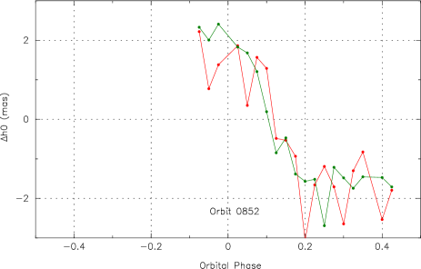
Figure 15: Drifting of the basic angle as observed in orbit 852, probably due to a restart of the on-board computer. The mean residuals over intervals of about 15 minutes are shown for the two fields of view, but for one of the two the sign was changed. Thus, what is shown is twice the correction to half the basic angle. In this orbit the basic angle correction drifted by 8 mas over a period of 5 hours.

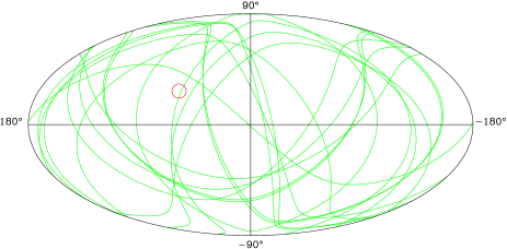
Figure 16: The distribution of orbits, in equatorial coordinates, that are affected by basic angle drift. The small circle shows the position and size of the Pleiades field.

The new reduction of the data allows further systematic checks to be made on the stability of the basic angle. These checks show generally a noise level that is below 0.2 mas. At that level it becomes impossible to distinguish real basic-angle variations from remaining systematics in the astrometric catalogue. In the new reduction, basic-angle drift corrections are only applied for orbits with clearly recognisable drift problems.

4.3 Conclusions on the basic-angle stability

The basic-angle stability for the Hipparcos mission was better than the requirements, except for fewer than one per cent of the orbits, most of which cover only half an orbit in data. The amount of data concerned is therefore very small, though for an individual star this does not need to be the case. The map of the great circles with basic angle drift shows some areas where up to 5 of these circles cross close together (Fig. 16). Correction of basic-angle drifts is often possible, though some loss of data quality is unavoidable for the most seriously affected orbits, as in these cases also the scale in the instrument parameters and the modulation parameters for the main grid are significantly affected.

5 Connectivity

The second requirement for the construction of absolute parallaxes, good connectivity between observations in the two fields of view, was generally assumed to have been taken care off by the construction of the Input Catalogue (ESA 1992) and the observing strategy. As was stated in the introduction, connectivity is obtained through the reconstruction of the along-scan attitude or scan phase. If the along-scan attitude reconstruction is based on one field of view only, it can adapt itself to “faulty” astrometry, such as a local offset of the parallax zero point. Only by ensuring that this reconstruction is based on (significant) contributions from observations in both fields of view it becomes possible to iterate out these local adjustments and obtain absolute parallaxes. The global tests on the parallax zero point and formal errors in the catalogue (Lindegren 1995; Arenou et al. 1995) indicate that this condition was largely fulfilled for most of the sky in the preparation of the Hipparcos catalogue, but there may have been exceptions in specific regions with a high density of bright stars, such as some open cluster centres (van Leeuwen 2005).

5.1 The Input Catalogue

The distribution of stars on the sky is not ideal for a mission like Hipparcos, given the high range of stellar densities even for its limiting magnitude (Hp=12). Limitations on the telemetry and as imposed by the observing technique meant that no more than around 120 000 stars could be observed by the mission. These 120 000 stars had to be selected from 214 000 stars requested in observing proposals. This task was assigned to the selection committee (led by Adriaan Blaauw) and the Input Catalogue consortium (led by Catherine Turon) (ESA 1989, 1992). The distribution of the requested stars reflects the main features of stellar density on the sky, such as the Milky Way and open clusters. The highest densities for the requested stars, as measured over 6.4 square degree fields, are about 50 times higher than the lowest densities. After selection the typical density range in the Input Catalogue is about a factor 10. The final selection consists of two parts (Turon et al. 1992):

• A survey of about 52 000 bright stars, which is complete to a limiting magnitude as a function of spectral type and galactic latitude;

• About 66 000 faint stars selected from the proposed observing programs.

The final selections were subjected to simulations to ensure that the expected astrometric accuracies were possible to obtain (Crézé in ESA 1989).

The selection was optimised on stellar density but not on integrated light. The remaining intensity contrasts on the sky are generally larger, as densely populated areas are often also areas with bright stars. The rigidity of the Hipparcos catalogue depends on how the reduction software has handled those contrasts, which in turn is determined by the formal errors assigned to observations in the great-circle reduction process. The input data for this process are the reduced frame transits, the grid-transit data collected for a star over a fixed 2.133 s period (roughly one ninth of a complete field-of-view transit). The modulation-phase estimates obtained for those transits have formal errors that reflect the signal modulation amplitude and Poisson statistics of the photon counts (see also Fig.9 in van Leeuwen & Fantino 2003). The only exceptions are the very brightest stars (Hp$<2.5$) where saturation disturbed the statistics. The relation between the formal error on the phase estimate and the integrated intensity for a transit is nearly constant for the mission. The main dependence is the relative amplitude of the first harmonic in the grid-modulated signal. The formal errors on the transit positions are given by:

$$\sigma_{a}\approx\frac{255}{M1\sqrt{I_{\mathrm{tot}}}}\leavevmode\nobreak\ \leavevmode\nobreak\ \leavevmode\nobreak\ \mathrm{mas},$$ (18)

where $I_{\mathrm{tot}}$ is the total photon count recorded for the transit, and $M1$ the relative amplitude of the first harmonic in the signal modulation. The main dependences of $M1$ are the focal adjustment of the telescope and the colour index of the observed star. The value of $M1$ generally varied between 0.6 (red stars) and 0.8 (blue stars).

For single frame transits $I_{\mathrm{tot}}$ ranges from a low of around 40 up to $10^{6}$ for the brightest stars.

Figure 17: Time variation of the response in the centre of the field for 8th mag stars of two different colour indices, showing the effect of aging of the detector chain through the decrease in response over the mission and the difference in this decrease for stars of different colour.

Equation 18 provides the photon-statistics limit on the formal errors which ideally propagates all the way to the final astrometry. When also using the second harmonic, as was done by the FAST consortium, the scaling coefficient is about 5 per cent smaller: the second-order amplitude is approximately 0.3 times the first harmonic amplitude, adding in weight 10 per cent to the solution, and reducing resulting formal errors by 5 per cent. These figures have been confirmed through extensive tests on the real data in the new reduction. Thus, when using the first and second harmonic, as was done in the FAST reductions, the factor in Eq. 18 becomes $\approx 242$ mas.

When the frame transits were used as input to the great-circle reduction, an assumed and fixed attitude noise was added in quadrature. The attitude noise at the frame transit level is generally around 3 mas. This means that above a total count of $10^{4}$ the attitude noise is dominant. In comparison, the response of an 8^th magnitude star over the mission is shown in Fig. 17. Thus, from approximately magnitude 6–7 the measurement noise as implemented for the great-circle reduction was the fixed attitude noise rather than the photon-count statistics. This reduced the effective total intensity contrasts between two fields of view in some cases considerably.

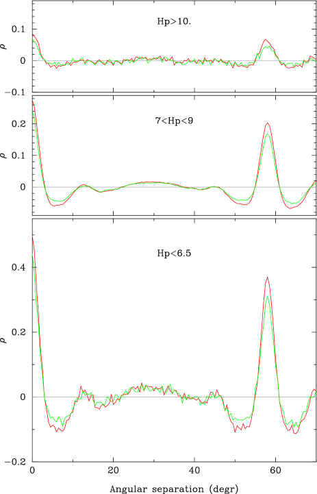
Figure 18: The zero- and first-order abscissa-error correlation peaks in the NDAC and FAST reductions for average length data sets and different magnitude ranges. The first-order peak shows the correlations introduced through the simultaneous measuring of stars from the two fields of view. The zero-order peak shows these correlations for stars at small separations. These correlations are the result of attitude errors, which reflect most strongly for bright stars for which the photon-noise contribution is relatively small.

The connectivity of the data and the contribution of the attitude noise show clearly from the abscissa-residual correlation statistics at orbit level. Average values for the whole mission have been presented in Volume 3 of ESA (1997) and by van Leeuwen & Evans (1998). However, averaged values are of limited use: the correlated errors originate from systematic errors in the along-scan attitude fitting, and these errors are much more dominant for bright stars than for faint ones (Fig. 18). Resolving the correlation statistics according to the magnitudes of the stars involved is not possible in detail, but an impression of correlation statistics when both stars fall in a given magnitude interval can be obtained. As one should expect, the correlations are considerably stronger for the bright-star pairs than for faint-star pairs. Tests with mixed magnitude pairs showed that the correlation statistics for these pairs is well represented by the statistics for the mean magnitude. The fact that significant correlations can still be observed even for stars of magnitude 10 and above is probably a reflection of the unresolved scan-phase jumps and hits in the published data, as it implies the presence of some systematic errors at a level of 5 mas and more. Applying the adjusted correlation statistics to the Pleiades parallax solution provides a new cluster-parallax estimate of approximately 8.0 mas (van Leeuwen 2005), about halfway between the earlier Hipparcos-based estimate and the “expected” value, and with a difference at about 1 sigma of the formal error on the newly derived Hipparcos-based parallax.

5.2 The weight contrast in the Input Catalogue

The typical weight of a given area on the sky, in comparison with other areas, gives a more accurate impression of the remaining contrasts in the Input Catalogue than comparing number densities of stars. These weights determine the relative influence an area of the sky can exert on the along-scan attitude determination. Assuming photon noise and attitude noise as described above, the intensities of stars are added rather than their numbers. The procedure is as follows. The Hp magnitudes of all catalogue stars within a 1$\aas@@fstack{\circ}$3 radius around each catalogue star are collected and transformed to pseudo intensities. To represent the modelling noise (mainly from the along-scan attitude reconstruction) all stars brighter than magnitude Hp$=7$ are treated as magnitude 7 stars. This is further referred to as the minimum magnitude. The intensities are added to obtain an integrated intensity. Thus, for each star we have available the number of stars within a 1$\aas@@fstack{\circ}$3 radius, and the integrated intensity for that area. While the number counts have a dynamic range of about 20, the intensities have a range of about 60 (Fig. 19). The highest intensities are found for the cores of open clusters, in particular NGC 3114 in Carina and the Pleiades. Lowering the attitude noise, as is the case in the new reductions, lowers the minimum magnitude and further increases the contrast.

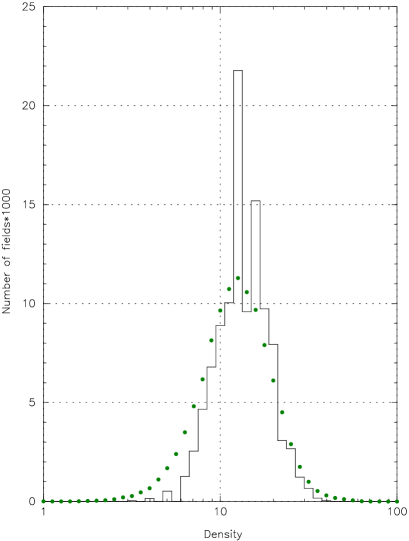
Figure 19: Histograms of the number of stars (line) and total intensity (dots) over 5.3 square-degrees fields centred on catalogue entries. The dynamic range (given by the width of the histogram) of the total intensity per field is significantly higher than for the total number of stars.

Within the principles of the Hipparcos mission more weight is not necessarily a good thing: areas with relatively high weight may not conform to the requirement of connectivity. The result can be that in such areas the fitting of the along-scan attitude is based almost entirely on the data from that one field of view, preventing it from proper attachment to the rest of the catalogue. This can lead locally to astrometric data for which the accuracy is not fully reliable. An apparently discrepant parallax determination, as has been suggested to be the case for the Pleiades, could be the result. The astrometry in these fields may be partially detached from the catalogue. As these fields rarely also contain stars at sufficiently large distances to be used as check on the parallax zero point, it is difficult to verify independently whether this is or is not a serious (local) problem in the Hipparcos data. There is one indication, however, that it possibly is not. It would be expected, given the independent reduction chains, for the results of such detached areas in the FAST and NDAC reductions to differ by more than the expected amount. When comparing a map of the parallax differences between the FAST and NDAC results with a map of the areas with high weight, there are at most a few marginal correlations. These comparisons indicate that the detachment due to excess weight may not play a very serious role in the reliability of the Hipparcos catalogue. There is one proviso that needs to be made here: the two consortia started reductions using the same Input Catalogue (ESA 1992), and used nearly the same data (the only differences being in stretches of data accepted or rejected). Local systematic errors due to detachment may possibly, as a result, have developed in a similar way.

5.3 Is re-attachment of detached areas possible?

It is to the credit of Valeri Makarov who first identified some of the effects described above as a possible reason for the problems experienced with the Pleiades parallax. Makarov also suggested and applied a method for correcting (re-connecting?) detached areas (Makarov 2002, 2003). A range of assumptions is made by Makarov about the way observations are distributed between the two fields of view. The availability of the raw data and a complete data analysis package allows checking those assumptions. The method of Makarov is based on the idea of incorporating the abscissa residuals from the other field of view to correct those of a potentially detached area. This idea had been first put forward by van Leeuwen (1999b), but its implementation was rejected on statistical grounds: for the field covering the centre of the Pleiades cluster the unit-weight variance of the potentially coinciding abscissa residuals was observed to be smaller than that of the non-coinciding residuals.

Makarov accumulated the data from great circles on which observations of a target area are contained, and selected the data from stars positioned on those circles at $58\pm 0.7$ degrees from the target field, the so-called coinciding stars. By assuming that all these coinciding stars had half of their observations coinciding with the target field, and half not, he argued that any systematic residual caused by the target field will on average equal half of the residual of the coinciding star for that circle. This translates into a correction coefficient $R=2$.

To check the validity of this correction coefficient, and using the raw data, a total of 1400 great circles were investigated, each containing the transits of at least 1000 different stars. For each star the potentially coinciding stars were selected, where a potentially coinciding star is situated at $58\pm 0.7$ degrees from the target star. Both the target star and the coinciding star have potentially observations in both fields of view, and in only one of those FOVs the measurements may coincide. This situation is represented by a statistical parameter $p$. If there are in total $n_{t}$ observations for the target star, and $n_{c}$ observations for the coinciding star, and there are $n_{k}$ coinciding observations, then:

$$p\equiv n_{k}/\sqrt{n_{t}\cdot n_{c}}$$ (19)

In an ideal situation, both stars have been observed the same number of times, equally distributed between the two FOVs, and half of these observations coincided with the other star. In that case, $p=0.5$. This is equivalent to setting $R=2$ in Makarov (2002). The data for several million actual field transits shows, however, that the real situation is far from ideal.

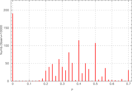
Figure 20: Distribution of the coincidence statistic $p$ for a large selection of stars, restricted to an ordinate difference of less than 0.75 degrees. The peak at $p=0$ represents the unsuccessful potentially-coinciding stars.

To start, 35 per cent of the potentially coinciding stars never have any coinciding measurements and can therefore be only indirectly correlated. Most of these missed chances are due to the ordinate differences between the target and the coinciding star. By limiting the ordinate difference to 0.75 degrees, only 13 per cent does not coincide. But for those that do coincide, the distribution over the statistic $p$ shows an efficiency that is well below the ideal value of 0.5 (see Fig. 20). The average value for $p$ in this selection is 0.32 (without the additional selection it is 0.26). The average value of $p$ will decrease with increasing length of the time interval covered by the great circle, as is also reflected in the correlation statistics by van Leeuwen & Evans (1998). Taking therefore all potentially coinciding stars as actually coinciding, and at the ideal distribution of observing time, seems highly unjustified.

The use of the abscissa residuals from coinciding transits has a further risk. The noise on those residuals is composed of two main contributions: Poisson and attitude noise. As was explained above, Poisson noise dominates for stars fainter than Hp$=8$, while attitude noise dominates for stars brighter than Hp$=6$. Transferring abscissa residuals from faint coinciding stars onto the target field will not be of any benefit for the target field, it will only increase the overall noise levels. The fact that a possibly more likely answer is found by Makarov using this method is no proof of the validity of the method. In fact, his method contradicts his probably correct assumption about the problem with the Pleiades parallax: when assuming that the Pleiades region is detached from the catalogue, it is not possible to correct it with methods that would apply only under condition of (nearly) ideal connectivity. On the other hand, if areas are ideally connected then there is no reason to apply a correction.

5.4 Conclusions on connectivity

Connectivity may have been a relatively minor issue in the construction of the Hipparcos catalogue, affecting only a few extreme areas of the sky. Unfortunately, these areas also tend to be some of the most interesting. However, when in a new reduction the attitude noise contribution is considerably reduced, the weight contrasts will increase and many more areas will be affected. This can be prevented by artificially damping the weight ratio between the two fields of view to a reasonable fraction. Even so it will still be necessary to iterate the solution to ensure full connectivity over the whole sky. Any effects of poor connectivity in the published catalogue cannot be corrected afterwards from the intermediate astrometric data. Connectivity is very relevant for the reduction of the astrometric data of the Gaia mission (Perryman 2002), where contrasts are purely set by the actual stellar density variations on the sky, and reach much higher values than encountered for the Hipparcos mission.

6 Some statistical properties resulting from the merging of the data

The great-circle reduction process and the associated potential for instabilities made a clean propagation of formal errors virtually impossible. In addition, the total integrated intensities of transits were not propagated through the reduction chain, thus a handle on those formal errors was effectively lost. This led to various “adjustments” of errors along the way: in the great-circle reduction results, the sphere reconstruction and the data merging. Some adjustments were made as a function of stellar magnitude, while observing-time variations implied that there was no clean direct relation between formal errors and those magnitudes. Most, but not all, features observed in the formal errors on the published (per-orbit) abscissae can be understood from the descriptions in Volume 3, Chapters 9, 11, 16 and 17 of ESA (1997).

6.1 Propagation of errors

As was stated before, the errors on the Hipparcos astrometry all originate from two sources: photon noise and modelling errors. The photon noise is a function of the integrated photon-count and the modulation amplitude $M1$, and reflects in the formal errors on the positional estimates as described by Eq. 18.

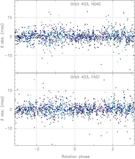
Figure 21: Abscissa residuals for the FAST and NDAC reductions of orbit 403. Some remaining systematics are still visible in both graphs.

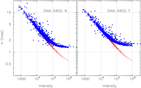
Figure 22: Formal errors as assigned to the abscissa residuals for orbit 403. The thin dots in the background give the formal errors for the new reduction, as based on the transit intensities and modulation amplitude of the first harmonic, $M1$.

The modelling noise consists of two main contributions: reconstruction of the along-scan phase (attitude) and reconstruction of the instrument parameters, describing the differential relations between positions on the sky and on the grid for the two fields of view and for stars of different colour indices. The first of these two generally dominates the modelling noise, and covers all the problems presented earlier in this paper: phase jumps, hits, eclipses and solution instabilities.

6.2 Statistical peculiarities of the merged data

The level of the attitude noise was set empirically, based on the observed variance of the abscissa residuals following the great-circle reduction. The attitude noise thus introduced varies strongly from data set to data set, between lows of 1.3 mas and highs of 10 mas. The high noise values always hide strong systematics in the residuals. An example of a typical good data set is shown in Fig. 21 and Fig. 22, with an attitude noise level for NDAC of 1.3 mas and for FAST 1.5 mas. The photon noise is observed close to the expected relation, slightly lower for FAST than for NDAC due to the inclusion of the second harmonic.

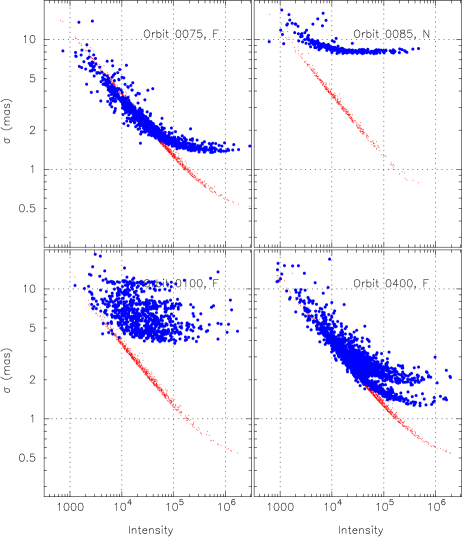
Figure 23: Peculiarities in the formal errors on abscissa residuals for some selected orbits (see text for details). N: NDAC, F: FAST

Several deviations from this more or less ideal situation are observed. Examples of some typical situations are shown in Fig. 23. The first example, orbit 75, top left, shows the effects of a single correction applied to the formal errors as part of the catalogue merging. As part of the merging process, the standard errors on the FAST and NDAC great-circle results were “normalised”. However, as at that stage information on the two noise components was no longer available, the “normalisation” was applied to all observations. As a result, it appears that noise levels significantly below the minimum photon noise are assigned to the fainter transits, which seems unrealistic. This situation occurs frequently for data sets from the first few months of the mission, as reduced by FAST.

The second example, orbit 85, top right, shows an extreme case of the attitude noise contribution. In this case the attitude noise hides large-scale systematics in the abscissa residuals for a short stretch of data, caused by the instabilities in the great-circle reduction described above. The attitude noise in these data sets is highly non-Gaussian.

The third example, orbit 100, bottom left, shows a situation that looks like multiple attitude noise levels having been applied to various short stretches of data. The cause of this behaviour is still unclear. It occurs, to various degrees of severity, in quite a few FAST data sets.

The final example, orbit 400, bottom right, shows a case where in the FAST reduction an orbit was split in two parts because of the presence of a large data gap (in this case the gap was just over one revolution of the satellite). Each part of the reduction was assigned an attitude noise level, and the two parts were later merged to one data set in the preparations for the merging of the FAST and NDAC data.

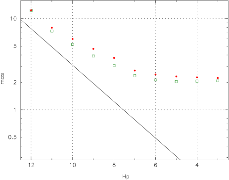
Figure 24: Standard deviations ($\sigma$ in mas) for the abscissa residuals as a function of the $\mathrm{H}p$ magnitude. Open symbols refer to FAST data, filled symbols to NDAC data. The diagonal line represents the expected relation for Poisson noise on the photon counts only, given identical integration times for all magnitudes. The flattening of the relation towards brighter magnitudes shows the 2 mas noise contribution from the instrument parameters and attitude modelling.

How these formal errors translated into dispersions of abscissa residuals as a function of magnitude is shown in Fig. 24. The initial departure from the photon-noise relation is mainly due to amounts of observing time assigned to stars of different magnitudes. The flattening towards the brighter stars shows the average attitude noise at orbit-transit level for the published data.

These statistical properties of the abscissa data imply that it is close to impossible to provide a reliable global abscissa-error correlation function for the Hipparcos data. Conditions differ from one orbit to the next. The same is probably also true of the correlation coefficients between the FAST and NDAC data. As a result, studies of astrometric parameters for open clusters are severely hampered by intrinsic uncertainties, which can no longer be solved a posteriori from the published data. The only reasonable way forward appears to be a complete re-reduction of the raw Hipparcos data, without the use of the great-circle reduction, but starting from the current published catalogue. Only that way can large-scale systematics and the associated abscissa error correlations as well as anomalous formal errors on the abscissae be eliminated.

7 Statistical verification of the astrometric data

The verification of a data set claiming a unique level of accuracy is always very difficult. For the Hipparcos data there were available a very limited number of parallaxes with compatible accuracies, and proper motions based on a very much longer base line than explored by Hipparcos. Positional reference frames in optical wavelengths as obtained with ground-based instrumentation suffer from systematic errors well beyond the accuracy level of the Hipparcos data. There is, however, a small number of radio sources with astrometric parameters of compatible accuracy.

Several tests have been applied to the Hipparcos data to test its reliability:

• Comparisons with any available astrometric data of compatible accuracy, in optical and radio wavelengths;

• Testing of formal errors and parallaxes for objects with negligible parallaxes, such as stars in the SMC and LMC;

• Comparing the distribution of negative parallaxes with the expected distribution for the given formal errors;

• Comparing globally parallaxes for open clusters with pre-Hipparcos estimates of their distances.

These tests were carried out by Lennart Lindegren and Frédéric Arenou (Lindegren 1995; Arenou et al. 1995), and indicated quite clearly that globally the parallaxes and formal errors formed a reliable and internally consistent data set. The independent tests by Arenou and Lindegren showed no systematic bias in the parallax zero point down to a level of 0.1 mas, and confirmed the formal errors to agree with actual errors to within 2 to 3 per cent.

There are some aspects of these tests that would warrant caution on their results. The first concerns the magnitude range (and thus the formal error range) for the tests. The tests are dominated by data for faint stars, with errors set by photon noise only. Bright stars are generally only suitable for comparisons with ground-based observations which tend to be of much lower accuracy than the Hipparcos data. As was shown above, potential connectivity problems are in particular relevant for the brighter stars.

There is also still a small problem with the proper motions of cluster members. Internal proper motion dispersions in open clusters have been studied on the basis of differential astrometry with 10 times higher precision than the Hipparcos data (see for example van Leeuwen 1994). For the core of the Pleiades this dispersion is about 0.8 mas $\mathrm{yr}^{-1}$. The internal dispersions in the open cluster proper motions as derived by van Leeuwen (1999a) and Robichon et al. (1999) from the Hipparcos data on the basis of the overall dispersion of the proper motions and their formal errors, are at a level of 1.5 to 2 mas $\mathrm{yr}^{-1}$, well above the expected values. Detailed problems with the proper motions of cluster stars are also indicated when comparing the differential components of the Pleiades proper motions as measured by Hipparcos with the best available differential determination by Vasilevskis et al. (1979). Given the distances of the clusters involved, this is unlikely to be an effect of unresolved orbital motions.

8 Conclusions

Above all, it should be recognised that the two data reduction consortia, in close collaboration with the ESA teams at ESOC and ESTEC, produced a Hipparcos catalogue with astrometric accuracies well exceeding the original aims and expectations of the mission, and did so under the very difficult conditions set by the orbit anomaly. Criticisms that have been expressed, concern the reliability of the catalogue for one or two small areas of the sky, where conditions for reconstructing the best possible astrometry may not have been sufficiently well understood during the data reductions. These aspects, and a range of other partly overlooked disturbances of the data, as well as the possibility of now sidestepping the great-circle reduction process, with its potential instabilities, still create opportunities for significant further improvements to the catalogue, in both overall accuracy and statistical reliability. As the Hipparcos data is irreplaceable, it is felt that this new reduction of the Hipparcos data needs to be done to preserve the best possible results from what has so far been a unique experiment. Furthermore, the experience obtained with the new analysis and reduction of the Hipparcos data is of direct benefit for the forthcoming Gaia mission, in particular concerning overall connectivity for the reconstructed astrometric catalogue and the importance of rigidity of the spacecraft for the along-scan attitude reconstruction.