Dynamical bar instability in a relativistic rotational core collapse

Abstract

We investigate the rotational core collapse of a rapidly rotating relativistic star by means of a 3+1 hydrodynamical simulations in conformally flat spacetime of general relativity. We concentrate our investigation to the bounce of the rotational core collapse, since potentially most of the gravitational waves from it are radiated around the core bounce. The dynamics of the star is started from a differentially rotating equilibrium star of $T/W\sim 0.16$ ($T$ is the rotational kinetic energy and $W$ is the gravitational binding energy of the equilibrium star), depleting the pressure to initiate the collapse and to exceed the threshold of dynamical bar instability. Our finding is that the collapsing star potentially forms a bar when the star has a toroidal structure due to the redistribution of the angular momentum at the core bounce. On the other hand, the collapsing star weakly forms a bar when the star has a spheroidal structure. We also find that the bar structure of the star is destroyed when the torus is destroyed in the rotational core collapse. Since the collapse of a toroidal star potentially forms a bar, it can be a promising source of gravitational waves which will be detected in advanced LIGO.

I Introduction

Rotational core collapse occurs in the first phase of the collapse-driven supernova explosion. The collapse takes place in a dynamical time scale and the bounce occurs when the central part of the star collapses into a nuclear density and then stiffens its equation of state. The final outcome of the collapse forms a compact object, such as a neutron star or a black hole, which is a candidate for sources of gravitational waves (Cutler and Thorne, 2002). There are two different approaches to investigate the rotational core collapse. One is to take into account the realistic picture of the rotational collapse such as realistic equation of state of the neutron star and/or neutrino effect in Newtonian gravity (e.g. Fryer and Heger, 2000; Kotake et al., 2003; Müller, Rampp, Buras, Janka, and Shoemaker, 2004). The other is to illustrate simplified physics in relativistic gravitation (e.g. Dimmelmeier, Font, and Müller, 2001, 2002). Since one of our aims in this paper is to investigate the possibility of gravitational wave sources in rotational core collapse, we should at least take into account relativistic gravitation, which significantly affects the quantitative behavior of gravitational waves from rotational core collapse (Cerda-Duran et al., 2004).

Dynamical bar instability in a rotating equilibrium star takes place when the ratio $\beta(\equiv T/W)$ between rotational kinetic energy $T$ and the gravitational binding energy $W$ exceeds the critical value $\beta_{\rm dyn}$. Determining the onset of the dynamical bar-mode instability, as well as the subsequent evolution of an unstable star, requires a fully nonlinear hydrodynamic simulation. Simulations performed in Newtonian gravity (e.g. Tohline, Durisen, and McCollough, 1985; Durisen et al., 1986; Williams and Tohline, 1988; Houser, Centrella, and Smith, 1994; Smith, Houser, and Centrella, 1996; Houser and Centrella, 1996; Toman et al., 1998; New, Centrella, and Tohline, 2000; Liu and Lindblom, 2001; Liu, 2002) have shown that $\beta_{\rm dyn}$ depends only very weakly on the stiffness of the equation of state. $\beta_{\rm dyn}$ becomes small for stars with high degree of differential rotation (Tohline and Hachisu, 1990; Pickett, Durisen, and Davis, 1996; Shibata, Karino, and Eriguchi, 2002). Simulations in relativistic gravitation (Shibata, Baumgarte, and Shapiro, 2000; Saijo et al., 2001) have shown that $\beta_{\rm dyn}$ decreases with the compaction of the star, indicating that relativistic gravitation enhances the bar-mode instability. The dynamical bar instability potentially occurs during the collapse since the nondimensional value $\beta$ scales as $R^{-1}$ in the dimensional analysis where $R$ is the radius of the star. Let us briefly discuss a picture of core bounce. When the star collapses, $\beta$ increases and the star starts to deform its shape to form a bar when the star exceeds the critical value of dynamical instability. During the bounce phase, $\beta$ falls below the threshold of dynamical instability, and the star cannot deform furthermore. In such a situation, what happens to the nonaxisymmetric deformation of the star?

There are several papers that investigate rotational core collapse as a potential source of gravitational waves in axisymmetric spacetime in Newtonian gravity (Zwerger and Müller, 1997; Kotake et al., 2003), in conformally flat spacetime (Dimmelmeier, Font, and Müller, 2001, 2002; Siebel et al., 2003), and in full general relativity (Stergioulas, Apostolatos, and Font, 2004; Shibata and Sekiguchi, 2004; Shibata04, ) to estimate the amount of gravitational radiation (Fryer, Holz and Hughes, 2002). Recently, 3D calculations in full general relativity have been established to investigate the nonaxisymmetric deformation of the star in rotational core collapse. Duez, Shapiro, and Yo (2004) investigated the collapse of a differentially rotating $n=1$ polytropic star in 3D by depleting the pressure and found that the collapsing star forms a torus which fragments into nonaxisymmetric clumps. Shibata and Sekiguchi (2005) investigated in rotational core collapse and found that a burst type of gravitational waves was emitted. In addition, they argued that a very limited window for the rotating star satisfies to exceed the threshold of dynamical instability in the core collapse. Zink et al. (2005) presented a fragmentation of an $n=3$ toroidal polytropic star to a binary system inducing $m=2$ density perturbation and claimed that they found a new scenario to form a binary black hole.

Our purpose in this paper is the following twofold. One is to investigate a necessary condition and mechanism to enhance the dynamical bar instability in a collapsing star. Brown (2001) performed long time integration of the rotational core collapse to investigate whether a dynamical bar can significantly form during the evolution. He found that the dynamical bar instability sets in at $\beta_{\rm dyn}\approx 0.23$, which is far below the standard value $\beta_{\rm dyn}\approx 0.27$. He found that the role of dynamical bar in rotational core collapse may be quite different from that in the equilibrium star. He also found that the bar instability grows slowly in core bounce. His finding can be interpreted that bar instability is initiated by the interaction between the core part and the surrounding part of the star. Therefore the “dynamical” bar instability in the collapsing star is quite different from that in the equilibrium state.

The other is the importance of probing whether the rotational core collapse becomes a promising source of gravitational waves. Direct detection of gravitational waves by ground based and space based interferometers is of great importance in general relativity, in astrophysics, and in cosmology. Once a bar has formed in the neutron star, we may expect quasi-periodic gravitational waves in the kHz band, which may be detectable in advanced LIGO (Cutler and Thorne, 2002). Rampp, Müller, and Ruffert (1998) investigated the rotational core collapse using parametric equation of state in Newtonian gravity, including the thermal pressure and the nuclear matter when the density exceeds the threshold of nuclear density. They found that although the rotating star has a nonaxisymmetric deformation, the amplitude of gravitational waves does not significantly grow during the deformation. In fact, they compared the gravitational waveform computed in their simulation with that in the previous 2D calculation (Zwerger and Müller, 1997) and found that it is quite similar to each other. Therefore, even if the nonaxisymmetric instability takes place during the collapse, the bar does not significantly grow at the core bounce. What else do we need to enhance the bar formation in the rotational core collapse?

Our interest is to focus on the core bounce of the rotational core collapse in order to investigate the angular momentum redistribution and to investigate the possibility of gravitational wave sources. Accordingly we construct a mimic model to investigate the above two issues. We deplete the pressure of the equilibrium star to initiate collapse and bounce. We also concentrate on the structure of the star, spheroidal and toroidal, to investigate the dynamical bar instability in the collapsing star. Stellar collapses and mergers may also lead to differentially rotating stars (e.g. Ott et al., 2004). For the coalescence of binary irrotational neutron stars (Shibata and Uryu, 2000, 2002; Shibata, Taniguchi, and Uryū, 2003), the presence of differential rotation may temporarily stabilize the “hypermassive” remnant, which constructs a toroidal structure and may therefore have important dynamical effects. Although they use stiff equation of state ($n=1$) it is possible to construct a toroidal star in nature.

This paper is organized as follows. In Sec. II we summarize our basic equation of relativistic hydrodynamics in conformally flat spacetime. In Sec. III we show our numerical results of dynamical bar instability in rotational core collapse, and summarize our findings in Sec. IV. Throughout this paper we use geometrized units ($G=c=1$) and adopt Cartesian coordinates $(x,y,z)$ with the coordinate time $t$. Greek and Latin indices run over $(t,x,y,z)$ and $(x,y,z)$, respectively.

II Relativistic Hydrodynamics in Conformally Flat Spacetime

In this section, we describe the basic equations in conformally flat spacetime (e.g. Isenberg and Nester, 1980; Wilson and Mathews, 1989; Saijo, 2004). We solve the fully relativistic equations of hydrodynamics, but neglect nondiagonal spatial metric components.

II.1 The gravitational field equations

We define the spatial projection tensor $\gamma^{\mu\nu}\equiv g^{\mu\nu}+n^{\mu}n^{\nu}$, where $g^{\mu\nu}$ is the spacetime metric, $n^{\mu}=(1/\alpha,-\beta^{i}/\alpha)$ the unit normal to a spatial hypersurface, and where $\alpha$ and $\beta^{i}$ are the lapse and shift. Within a first post-Newtonian approximation, the spatial metric $g_{ij}=\gamma_{ij}$ may always be chosen to be conformally flat

$$\gamma_{ij}=\psi^{4}\delta_{ij},$$ (1)

where $\psi$ is the conformal factor (see Chandrasekhar, 1965; Blanchet, Damour, and Schäfer, 1990). The spacetime line element then reduces to

$$ds^{2}=(-\alpha^{2}+\beta_{k}\beta^{k})dt^{2}+2\beta_{i}dx^{i}dt+\psi^{4}\delta_{ij}dx^{i}dx^{j}.$$

We adopt maximal slicing, for which the trace of the extrinsic curvature $K_{ij}$ vanishes,

$$K\equiv\gamma^{ij}K_{ij}=0.$$ (3)

The gravitational field equations in conformally flat spacetime for the five unknown $\alpha$, $\beta^{i}$, and $\psi$ can then be derived conveniently from the 3+1 formalism. The equation for the lapse $\alpha$, shift $\beta^{i}$, and conformal factor $\psi$ with a maximal slicing implies $\partial_{t}K=0$, shall be written as

$$\triangle(\alpha\psi)=2\pi\alpha\psi^{5}(\rho_{\rm H}+2S)+\frac{7}{8}\alpha\psi^{5}K_{ij}K^{ij},$$ (4)

$$\delta_{il}\triangle\beta^{l}+\frac{1}{3}\partial_{i}\partial_{l}\beta^{l}=16\pi\alpha J_{i}+\left(\partial_{j}\ln\left(\frac{\alpha}{\psi^{6}}\right)\right)\left(\partial_{i}\beta^{j}+\delta_{il}\delta^{jk}\partial_{k}\beta^{l}-\frac{2}{3}\delta_{i}^{j}\partial_{l}\beta^{l}\right),$$ (5)

$$\triangle\psi=-2\pi\psi^{5}\rho_{\rm H}-\frac{1}{8}\psi^{5}K_{ij}K^{ij},$$ (6)

where $S=\gamma_{jk}T^{jk}$, $\Delta\equiv\delta^{ij}\partial_{i}\partial_{j}$ is the flat space Laplacian and $J_{i}\equiv-n^{\mu}\gamma^{\nu}_{~{}i}T_{\mu\nu}$ is the momentum density. In the definition of $J_{i}$, $T_{\mu\nu}$ is the stress energy tensor, $\rho_{\rm H}\equiv n^{\mu}n^{\nu}T_{\mu\nu}$ is the mass-energy density measured by a normal observer.

II.2 The matter equations

For a perfect fluid, the energy momentum tensor takes the form

$$T^{\mu\nu}=\rho\left(1+\varepsilon+\frac{P}{\rho}\right)u^{\mu}u^{\nu}+Pg^{\mu\nu},$$ (7)

where $\rho$ is the rest-mass density, $\varepsilon$ the specific internal energy, $P$ the pressure, and $u^{\mu}$ the four-velocity. We adopt a $\Gamma$-law equation of state in the form

$$P=(\Gamma-1)\rho\varepsilon,$$ (8)

where $\Gamma$ is the adiabatic index which we set $\Gamma=5/3$, $3/2$, $7/5$ in this paper. In the absence of thermal dissipation, Eq. (8), together with the first law of thermodynamics, implies a polytropic equation of state

$$P=\kappa\rho^{1+1/n},$$ (9)

where $n=1/(\Gamma-1)$ is the polytropic index and $\kappa$ is a constant.

From $\nabla_{\mu}T^{\mu\nu}=0$ together with the equation of state (Eq. [8]), we can derive the energy and Euler equations according to

$$\frac{\partial e_{*}}{\partial t}+\frac{\partial(e_{*}v^{j})}{\partial x^{j}}=-\frac{1}{\Gamma}(\rho\epsilon)^{-1+1/\Gamma}P_{\rm vis}\frac{\partial}{\partial x^{i}}(\alpha u^{t}\psi^{6}v^{i}),$$ (10)

$$\frac{\partial(\rho_{*}\tilde{u}_{i})}{\partial t}+\frac{\partial(\rho_{*}\tilde{u}_{i}v^{j})}{\partial x^{j}}=-\alpha\psi^{6}(P+P_{\rm vis})_{,i}-\rho_{*}\alpha\tilde{u}^{t}\alpha_{,i}+\rho_{*}\tilde{u}_{j}\beta^{j}_{~{},i}+\frac{2\rho_{*}\tilde{u}_{k}\tilde{u}_{k}}{\psi^{5}\tilde{u}^{t}}\psi_{,i},$$ (11)

where

$$e_{*} = (\rho\varepsilon)^{1/\Gamma}\alpha u^{t}\psi^{6},$$ (12)

$$v^{i} = {dx^{i}\over dt}=\frac{u^{i}}{u^{t}},$$ (13)

$$\rho_{*} = \rho\alpha u^{t}\psi^{6},$$ (14)

$$\tilde{u}^{t} = (1+\Gamma\varepsilon)u^{t},$$ (15)

$$\tilde{u}_{i} = (1+\Gamma\varepsilon)u_{i},$$ (16)

and $v^{i}$, $u^{\mu}$, $P_{\rm vis}$ is the 3-velocity, 4-velocity, pressure viscosity, respectively. Note that we treat the matter fully relativistically; the conformally flat approximation only enters through simplifications in the coupling to the gravitational fields. As a consequence to treat shocks we also need to solve the continuity equation

$$\frac{\partial\rho_{*}}{\partial t}+\frac{\partial(\rho_{*}v^{i})}{\partial x^{i}}=0,$$ (17)

separately.

Table 1: Relativistic Rotating Equilibrium stars

Model	$n$	$\hat{A}$	$R_{p}/R_{e}$	$\rho_{0}^{\rm max}$	$R_{c}$	$M$	$J$	$T/W$	$R_{c}/M$	$P_{\rm dep}$
I-a	$1.5$	$0.5$	$0.467$	$8.26\times 10^{-4}$	$6.56$	$1.64\times 10^{-1}$	$4.49\times 10^{-2}$	$1.59\times 10^{-1}$	$3.99\times 10^{1}$	$70\%$
I-b	$1.5$	$0.8$	$0.467$	$1.36\times 10^{-3}$	$7.22$	$1.79\times 10^{-1}$	$5.25\times 10^{-2}$	$1.59\times 10^{-1}$	$4.04\times 10^{1}$	$70\%$
II-a	$2.0$	$0.5$	$0.450$	$1.10\times 10^{-4}$	$2.53\times 10^{1}$	$6.29\times 10^{-1}$	$6.33\times 10^{-1}$	$1.63\times 10^{-1}$	$4.03\times 10^{1}$	$60\%$
II-b	$2.0$	$0.6$	$0.417$	$2.19\times 10^{-4}$	$2.64\times 10^{1}$	$6.62\times 10^{-1}$	$6.69\times 10^{-1}$	$1.62\times 10^{-1}$	$3.98\times 10^{1}$	$60\%$
III-a	$2.5$	$0.3$	$0.417$	$1.05\times 10^{-5}$	$8.63\times 10^{1}$	$2.16$	$6.90$	$1.59\times 10^{-1}$	$3.99\times 10^{1}$	$50\%$
III-b	$2.5$	$0.42$	$0.417$	$2.24\times 10^{-5}$	$8.54\times 10^{1}$	$2.13$	$6.58$	$1.60\times 10^{-1}$	$4.00\times 10^{1}$	$50\%$

II.3 Numerical techniques for solving gravitational field equations

We have reduced Einstein equations in conformally flat spacetime to ten elliptic equations for ten variables ($B_{i}$, $\chi$, $\psi$, $\alpha\psi$, $P_{i}$, $\eta$) using the same techniques in the previous paper (Saijo, 2004)

$$\Delta B_{i} = 8\pi\psi^{6}J_{i}\equiv 4\pi S_{B_{i}},$$ (18)

$$\Delta\chi = -8\pi\psi^{6}J_{i}x^{i}\equiv 4\pi S_{\chi},$$ (19)

$$\Delta\psi = -2\pi\psi^{5}\rho_{\rm H}-\frac{1}{8}\psi^{-7}\hat{A}_{ij}\hat{A}^{ij}\equiv 4\pi S_{\psi},$$ (20)

$$\Delta(\alpha\psi) = 2\pi\alpha\psi(\rho_{\rm H}+2S)+\frac{7}{8}\alpha\psi^{-7}\hat{A}_{ij}\hat{A}^{ij}$$ (21)

$$\equiv 4\pi S_{\alpha\psi},$$

$$\Delta P_{i} = 4\pi\alpha\hat{J}_{i}\equiv 4\pi S_{P_{i}},$$ (22)

$$\Delta\eta = -4\pi\alpha\hat{J}_{i}x^{i}\equiv 4\pi S_{\eta}.$$ (23)

We use the asymptotic fall off behavior for metric quantities at large radius in order to set an appropriate boundary condition at the grid edge (Saijo, 2004). The definition of $B_{i}$, $\chi$, $P_{i}$, $\eta$ and the basic procedure to solve ten elliptic equations are given in Ref. (Saijo, 2004). Since we parallelized our code, we change the method to solve the elliptic equation to PCG method (e.g. Murata, Natori, and Karaki, 1990).

We monitor the rest mass $M_{0}$, gravitational mass $M$, and the angular momentum $J$

$$M_{0} = \int\rho_{*}d^{3}x,$$ (24)

$$M = -\frac{1}{2\pi}\oint_{\infty}\nabla^{i}\psi dS_{i}$$ (25)

$$= \int\biggl{[}\left[(\rho+\rho\varepsilon+P)(\alpha u^{t})^{2}-P\right]\psi^{5}$$

$$+\frac{1}{16\pi}\psi^{5}K_{ij}K^{ij}\biggl{]}d^{3}x,$$

$$J = -\frac{1}{2\pi}\oint_{\infty}(xK^{j}_{y}-yK^{j}_{x})\psi^{6}dS_{i}$$ (26)

$$= \int(xJ_{y}-yJ_{x})\psi^{6}d^{3}x,$$

during the evolution. We also compute rotational kinetic energy $T$, proper mass $M_{p}$, gravitational binding energy $W$ as

$$M_{p} = \int\rho u^{t}(1+\epsilon)\sqrt{-g}d^{3}x$$ (27)

$$= \int\rho_{*}(1+\varepsilon)d^{3}x,$$

$$T = \frac{1}{2}\int\Omega T^{t}_{\phi}\sqrt{-g}d^{3}x$$ (28)

$$= \frac{1}{2}\int\Omega(xJ_{y}-yJ_{x})\psi^{6}d^{3}x,$$

$$W = M_{p}+T-M,$$ (29)

where $\Omega$ the angular velocity of the star.

Since we use a polytropic equation of state at $t=0$, it is convenient to rescale all quantities with respect to $\kappa$. Since $\kappa^{n/2}$ has dimensions of length, we introduce the following nondimensional variables (e.g. Cook, Shapiro, and Teukolsky, 1992)

$$\begin{array}[]{c c c}\bar{t}=\kappa^{-n/2}t,&\bar{x}=\kappa^{-n/2}x,&\bar{y}=\kappa^{-n/2}y,\\ \bar{z}=\kappa^{-n/2}z,&\bar{\Omega}=\kappa^{n/2}\Omega,&\bar{M}=\kappa^{-n/2}M,\\ \bar{R}=\kappa^{-n/2}R,&\bar{J}=\kappa^{-n}J.&\end{array}$$ (30)

Henceforth, we adopt nondimensional quantities, but omit the bars for convenience (equivalently, we set $\kappa=1$).

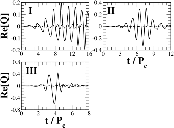
Figure 1: Evolution of quadrupole diagnostics in 6 different collapsing stars. Roman character in the panel corresponds to the model type in Table 1. Solid lines and dash lines represent toroidal and spheroidal stars, which correspond to model $a$ and $b$ in Table 1, respectively.

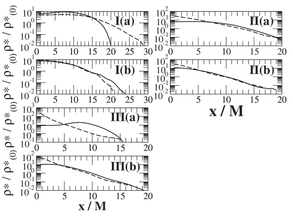
Figure 2: Snapshot of the coordinate density along the $x$-axis for 6 different stars (see Table 1). Solid lines and dash lines represent $t/P_{\rm c}=$ I(a) (9.61, 16.0), I(b) (9.67, 15.3), II(a) (2.39, 12.0), II(b) (3.25, 12.0), III(a) (3.19, 7.77), III(b) (3.20, 7.77), respectively.

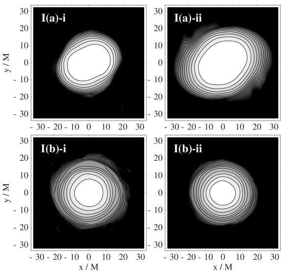
Figure 3: Density contour in the equatorial plane of 2 collapsing stars (Model I[a] and [b] of Table 1). Snapshots are plotted at the parameter ($t/t_{\rm dyn}$, $\rho^{*}_{\rm max}$) $=$ I(a)-i ($9.61$, $9.13\times 10^{-3}$), I(a)-ii ($16.0$, $6.04\times 10^{-3}$), I(b)-i ($9.67$, $1.33\times 10^{-2}$), I(b)-ii ($15.3$, $1.57\times 10^{-2}$), respectively. The contour lines denote coordinate densities $\rho^{*}=\rho^{*}_{\rm max}\times 10^{-0.220(16-i)}(i=1,\cdots,15)$.

Our code is based on the conformally flat hydrodynamics scheme of Ref. Saijo (2004), to which the reader is referred for a more detailed description, discussion and test. We choose the axis of rotation to align with the $z$ axis, and assume planar symmetry across the equator. The equations of hydrodynamics are then solved on a uniform grid of size $200\times 200\times 60$. We terminate our simulations after a sufficient number of central rotation periods (between 8 and 16) in order for us to detect dynamical instabilities. Because of our flux-conserving difference scheme the rest mass $M_{0}$ is conserved up to a round-off error, except if matter leaves the computational grid (which was never more than 0.01% of the total rest mass). In all cases reported in Sec. III the total gravitational mass $M$ and the angular momentum $J$ were conserved up to $\sim 0.1\%$ and less than about $5\%$ of their initial values.

III Rotational Core Collapse

We basically follow the scheme of Ref. (Komatsu, Eriguchi, and Hachisu, 1989) to construct a differentially rotating equilibrium star. The detailed procedure we used for constructing it is given in Ref. (Saijo, 2004). We construct the equilibrium star under the condition of fixing $\beta$ and $R_{\rm c}/M$, where $R_{\rm c}$ is the circumferential radius. This is because we keep approximately the same condition to extend the threshold of dynamical bar instability by depleting the pressure of the star to initiate collapse. We set one toroidal star (corresponds to model a in Table 1) and one spheroidal star (corresponds to model b in Table 1) for each polytropic index to focus on the structure of the star.

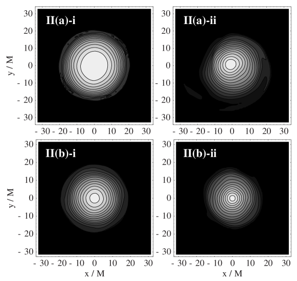
Figure 4: Density contour in the equatorial plane of 2 collapsing stars (Model II[a] and [b] of Table 1). Snapshots are plotted at the parameter ($t/t_{\rm dyn}$, $\rho^{*}_{\rm max}$) $=$ II(a)-i ($3.19$, $1.13\times 10^{-3}$), II(a)-ii ($12.0$, $4.62\times 10^{-3}$), II(b)-i ($3.25$, $3.39\times 10^{-3}$), II(b)-ii ($12.0$, $8.71\times 10^{-3}$), respectively. The contour lines denote coordinate densities $\rho^{*}=\rho^{*}_{\rm max}\times 10^{-0.200(16-i)}(i=1,\cdots,15)$.

We choose the rotation profile of the star as (Komatsu, Eriguchi, and Hachisu, 1989)

$$u^{t}u_{\varphi}=A^{2}(\Omega_{c}-\Omega),$$ (31)

which represents in the Newtonian limit ($u^{t}\rightarrow 1$, $u_{\varphi}\rightarrow\varpi^{2}\Omega$), so-called $j$-constant law, as

$$\Omega=\frac{A^{2}\Omega_{\rm c}}{\varpi^{2}+A^{2}},$$ (32)

where $A$ is a parameter representing the degree of differential rotation, $\varpi$ is the cylindrical radius of the star. Since $A$ has a dimension of length, we normalize it with the proper equatorial radius $\bar{R}_{e}$, ($A=\bar{R}_{e}\hat{A}$). We summarize our 6 different initial data sets of relativistic rotating equilibrium stars in Table 1.

To monitor the development of $m=2$ modes we compute a “quadrupole diagnostic” (Saijo, Baumgarte, and Shapiro, 2003)

$$Q=\left<e^{im\varphi}\right>_{m=2}=\frac{1}{M_{0}}\int\rho_{*}\frac{(x^{2}-y^{2})+i(2xy)}{x^{2}+y^{2}}d^{3}x,$$ (33)

where a bracket denotes the density weighted average. In the following we only plot the real parts of $Q$.

To enhance any $m=2$ instability, we disturb the initial equilibrium density $\rho_{\rm eq}$ by a nonaxisymmetric perturbation:

$$\rho=\rho_{\rm eq}\left(1+\delta\frac{x^{2}-y^{2}}{R_{\rm eq}^{2}}\right),$$ (34)

with $\delta=0.01$ in all our simulations.

As for computing the gravitational waveform, we use the same method that we used in the previous paper (Saijo et al., 2001). For observers along the rotational axis ($z$-axis), we have

$$\frac{rh_{+}}{M} = \frac{1}{2M}\frac{d^{2}}{dt^{2}}(I_{xx}-I_{yy}),$$ (35)

$$\frac{rh_{\times}}{M} = \frac{1}{M}\frac{d^{2}}{dt^{2}}I_{xy},$$ (36)

where $h_{+}$ and $h_{\times}$ are the two polarization modes of gravitational waves, $r$ is the distance to the source, $I_{ij}$ the approximate quadrupole moment of the mass distribution defined as

$$I_{ij}=\int\rho_{*}x^{i}x^{j}d^{3}x.$$ (37)

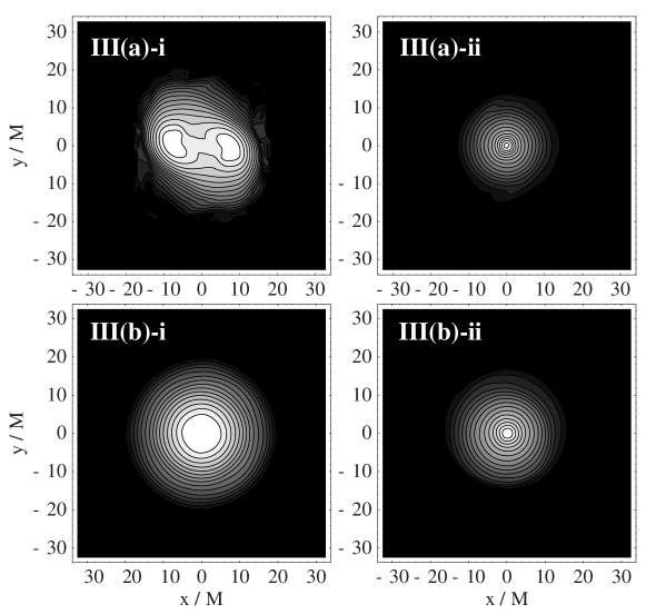
Figure 5: Density contour in the equatorial plane of 2 collapsing stars (Model III[a] and [b] of Table 1). Snapshots are plotted at the parameter ($t/t_{\rm dyn}$, $\rho^{*}_{\rm max}$) $=$ III(a)-i ($3.19$, $2.70\times 10^{-4}$), III(a)-ii ($7.77$, $4.02\times 10^{-3}$), III(b)-i ($3.20$, $3.28\times 10^{-4}$), III(b)-ii ($7.77$, $1.92\times 10^{-3}$), respectively. The contour lines denote coordinate densities $\rho^{*}=\rho^{*}_{\rm max}\times 10^{-0.220(16-i)}(i=1,\cdots,15)$.

We show the quadrupole diagnostic $Q$ throughout the evolution in Fig. 1. We determine that the system is stable to $m=2$ mode when the quadrupole diagnostic remains small throughout the evolution. We also determine that the system is unstable when the diagnostic grows exponentially at its early stage of evolution. It is clearly shown in Fig. 1 that the star is more unstable to the bar mode when the structure of the star is toroidal at its equilibrium stage than when it is spheroidal. Even in a spheroidal case, the dynamical instability sets in after the core bounce in case of model I(b) (see Table 1). Note also that the diagnostic damps out especially for the soft equation of state ($n=2$, $2.5$). The above effect corresponds to the destruction of the toroidal structure of the star (see Fig. 2).

We show the density contour in the intermediate stage and in the final stage of the rotational core collapse in Figs. 3 – 5. In the intermediate stage of the rotational core collapse, the bar instability grows due to the nonaxisymmetric instability. The deformation rate of the bar is significantly higher for the case of a toroidal star at equilibrium than that of a spheroidal star. At the termination of integration, the equatorial shape of the star is almost spherical except for the case of model I(a). The coincidence of the destruction of the toroidal structure in Fig. 2 at the termination of integration indicates that the structure of torus plays a significant role in enhancing bar instability.

We show the gravitational waveforms along the observer in the rotational axis in Fig. 6. The gravitational waves amplify during the bar formation. Since the dynamical bar plays an important role in our case of rotational core collapse, our result is quite different from the previous picture of the 3D Newtonian results (Rampp, Müller, and Ruffert, 1998). In fact, the amplitude in our calculation observed from the rotational axis grows about 20 times larger than that of core bounce which has a peak in the waveform. Note also that the quasiperiodic waves retain several rotation periods for stiff equation of state, due to the persistence of the toroidal structure.

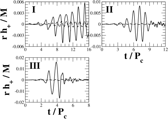
Figure 6: Gravitational waveforms from a distant observer along the rotational axis of the equilibrium star. Roman character in the panel corresponds to the model type in Table 1. Solid lines and dash lines represent toroidal and spheroidal stars, which correspond to $a$ and $b$ in Table 1, respectively.

We also show $\beta$ in the evolution in Fig. 7, which is regarded as a diagnostic of the dynamical bar instability in the equilibrium star. Although $\beta$ behaves quite similar in the different polytropic index, the bar structure persists for at least several rotation periods in case of the model I(a), which corresponds to the persistence of the toroidal structure (see Fig 2). We also show the distribution of the angular velocity in the intermediate stage and at the termination of the integration in Fig. 8. A sharp dip at the center in the angular velocity of model I(a) at $t=9.61P_{\rm c}$ potentially has a redistribution of the angular momentum.

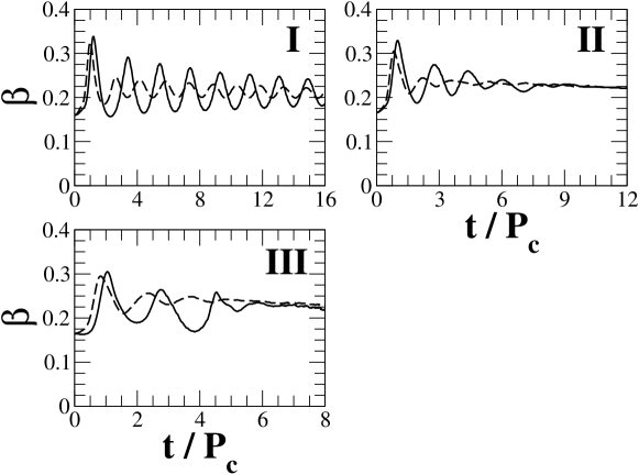
Figure 7: Diagnostics of dynamical bar instability $\beta$ as a function of time. Roman character in the panel corresponds to the model type in Table 1. Solid lines and dash lines represent toroidal and spheroidal star, which corresponds to $a$ and $b$ in Table 1.

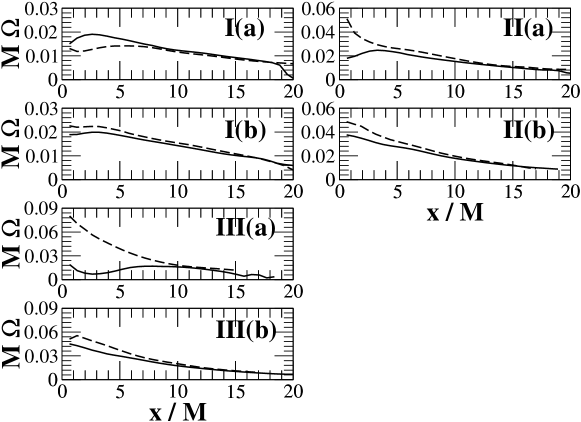
Figure 8: Snapshot of the orbital angular velocity along the $x$-axis. Solid lines and dash lines represent $t/P_{\rm c}=$ I(a) (9.61, 16.0), I(b) (9.67, 15.3), II(a) (2.39, 12.0), II(b) (3.25, 12.0), III(a) (3.19, 7.77), III(b) (3.20, 7.77), respectively.

IV Discussion

We investigate the role of dynamical bar instability in rotational core collapse by means of hydrodynamic simulations in conformally flat approximation in general relativity. We specifically focus on the structure of the star to see whether it takes a significant role in enhancing dynamical bar instability.

We find that the structure of the star takes a significant role in enhancing the dynamical bar instability at core bounce. Since the angular velocity of the collapsing star has already reached the maximum inside a certain cylindrical radius to produce a toroidal structure, the angular momentum can only shift outward at the bounce. For a spheroidal star, the angular momentum can shift both inward and outward at bounce since it does not reach the “Keplarian”. This means that rotational core collapse for the spheroidal case cannot significantly break the central core of the star. Consequently, in case of a toroidal star a bar structure is easily constructed during the evolution. Note that for a soft equation of state ($n=2.0$, $2.5$) the amplitude of gravitational waves decreases, as the torus is destroyed in the rotational core collapse. Therefore the torus is the key issue to trigger the bar formation.

Once a bar has formed, the amplitude of gravitational waves has significantly increased due to the nonaxisymmetric deformation of the star. The previous 2D calculation shows that a peak amplitude of gravitational waves comes from the core bounce of the star, and its behavior coincides with that of 3D calculation. In our results, gravitational radiation is dominantly generated in the bar formation process. Our results of the soft equation of state qualitatively agree with the results in full general relativity (Shibata and Sekiguchi, 2005). Thus, the characteristic amplitude and frequency of gravitational waves in the collapsing star can be written as

$$f_{\rm gw} \approx \frac{1}{2\pi t_{\rm dyn}}=100~{}[{\rm Hz}]\left(\frac{M_{\odot}}{M}\right)\left(\frac{40M}{R}\right)^{3/2},$$ (38)

$$h_{\rm gw} \approx 4.8\times 10^{-23}\left(\frac{M}{M_{\odot}}\right)\left(\frac{10{\rm Mpc}}{d}\right)\left(\frac{rh/M}{0.01}\right).$$

Therefore, gravitational waves from a dynamical bar in a collapsing neutron star will be detected in advanced LIGO.

Table 2: Magnitude of higher order correction for the central lapse at bounce

Model	${t_{\rm bce}/P_{\rm c}}$	$\alpha_{\rm c}$	$M_{\rm src}/R_{\rm src}$	$(M_{\rm src}/R_{\rm src})^{3}[\%]$
I-a	$1.22$	$0.872$	$0.137$	$0.257$
I-b	$1.00$	$0.848$	$0.166$	$0.457$
II-a	$1.05$	$0.843$	$0.172$	$0.509$
II-b	$0.88$	$0.806$	$0.218$	$1.04$
III-a	$1.08$	$0.835$	$0.181$	$0.593$
III-b	$0.90$	$0.803$	$0.222$	$1.09$

Finally we mention the validity of the conformally flat approximation in our 6 different collapsing stars. The approximation has two issues: that it contains the first post-Newtonian order of general relativity, and that it neglects gravitational radiation. First, we investigate the central lapse $\alpha_{\rm c}$ at core bounce to check whether the first post-Newtonian order of general relativity is reasonable approximation in our model. The central lapse can be expanded by the compaction (characteristic mass $M_{\rm src}$ and radius $R_{\rm src}$) of the source [Eq. (19.13) of Ref. (Misner, Thorne, and Wheeler, 1973)] as

$$\alpha_{\rm c}=1-\frac{M_{\rm src}}{R_{\rm src}}+\frac{1}{2}\left(\frac{M_{\rm src}}{R_{\rm src}}\right)^{2}+o\left(\left(\frac{M_{\rm src}}{R_{\rm src}}\right)^{3}\right).$$ (40)

Note that the shift appears in the $g_{tt}$ component of the 4-metric at the second post-Newtonian order of general relativity. All models of our 6 collapsing stars bounce at $\alpha_{\rm c}\gtrsim 0.8$, and therefore the value of central lapse corresponds to the compaction of the source $M_{\rm src}/R_{\rm src}\lesssim 0.22$ from Eq. (40). For each model, we summarize the magnitude of higher order correction [$(R_{\rm src}/M_{\rm src})^{3}$ term] from the first post-Newtonian order in Table 2. Note that the central lapse at bounce is the minimal one throughout the evolution. Since the magnitude of the higher order correction is $(M_{\rm src}/R_{\rm src})^{3}\lesssim 0.011$, we can roughly claim that the first post-Newtonian gravity is a satisfactory approximation to describe the full general relativity in the relative error rate of few percent in our calculation, depending on the coefficient of the higher order term. Second, it is also a quite satisfactory approximation to neglect gravitational radiation in our dynamics, since our main target in this paper is to focus on the enhancement of the dynamical bar instabilities which occur in dynamical time scale. Gravitational waves affect the whole dynamics in secular time scale, which is much longer than the dynamical time scale, and hence we can safely neglect such effect in this paper. Therefore, conformally flat approximation is a satisfactory one in our computation.