The Monopole Moment of the Three-Point Correlation Function of the 2-degree Field Galaxy Redshift Survey

Abstract

We measure the monopole moment of the three-point correlation function on scales $1\rm{h^{-1}Mpc}-70\rm{h^{-1}Mpc}$ in the Two degree Field Galaxy Redshift Survey (2dFGRS). Volume limited samples are constructed using a series of integral magnitudes bins between $M=-18\ldots-22$. Our measurements with a novel edge-corrected estimator represent most, if not all, three-point level monopole or angular averaged information in the catalogue. We fit a perturbative non-linear bias model to a joint data vector formed from the estimated two- and three-point correlation functions. Two different models are used: an analytic model based on Eulerian perturbation theory including bias and redshift distortions, and a phenomenological bias model based on the direct redshift space measurements in the large Virgo simulations. To interpret the clustering results, we perform a three parameter Gaussian maximum likelihood analysis. In the canonical $-21\sim-20$ volume limited sample we find $\sigma_{8}=0.93^{+0.06}_{-0.2}$, $b=1.04^{+0.23}_{-0.09}$, and $b_{2}=-0.06^{+0.003}_{-0.001}$. Our estimate of $\sigma_{8}$, is robust across the different volume limited samples constructed. These results, based solely on the large scale clustering of galaxies, are in excellent agreement with previous analyses using the Wilkinson Anisotropy Probe: this is a spectacular success of the concordance model. We also present two-parameter fits for the bias parameters, which are in excellent agreement with previous findings of the bias evolution in the 2dFGRS.

1 Introduction

Statistical analyses of the Two Degree Field Galaxy Redshift Survey (2dFGRS) (Colless et al., 2001) have propelled significant progress in high precision cosmology. For instance, measurements of the two-point correlation function and the power spectrum have provided tight constraints on the theories of structure formation (e.g. Percival et al., 2001; Norberg et al., 2001; Hawkins et al., 2003; Cole et al., 2005). The large volume and high quality of the 2dFGRS encourage further studies of higher order statistics. Such investigations provide information on the Gaussianity of the small initial dark matter fluctuations, the emergence of non-Gaussianity through non-linear gravitational effects, and even the murky physical processes of galaxy formation. The latter might manifest itself as “bias” (Kaiser, 1984), where the clustering of galaxies might be statistically different from that of the dark matter. Higher than second order statistics provide the only tool with which to separate these effects from the gravitational amplification and initial conditions. The resulting constraints on the bias are interesting in their own right, and they provide the new avenues to ultimately constrain cosmological parameters.

Third order statistics represent the first non-trivial step in the perturbative understanding of non-Gaussianity. Indeed, to date numerous works have been devoted mainly to the measurement and understanding of the third order statistics of 2dFGRS. Verde et al. (2002) estimated bias parameters from their bispectrum measurement at wave lengths $0.1<k<0.5{\rm h/Mpc}$. Three point correlation function $\zeta$ of an early released 2dF sample (2dF100k) is measured by Jing & Börner (2004) focusing on empirical formula fit for $\zeta$. Wang et al. (2004) measured three point correlation function for the 2dFGRS on small scales to test their conditional luminosity function model jointly with the halo model. As an alternative to the three-point correlation function or bispectrum, Croton et al. (2004) calculated moments of counts in cells, or averaged $N$-point correlation functions, on $1-9\rm{h^{-1}Mpc}$ scales, and estimated relative bias parameters.

A common thread in previous measurements was that they focused on either relatively small scales and/or a set of hand picked subset of triangular configurations, which characterize three-point statistics. With the most natural parametrizations predominantly used in the past, such as the three sides of a triangle $\zeta(r_{1},r_{2},r_{3})$, or $\zeta(r_{1},r_{2},\theta)$ with $\theta$ the angle between $r_{1}$ and $r_{2}$, it is both computationally burdensome, and conceptually difficult to measure and interpret three-point statistics in a large dynamic range. Recently, Szapudi (2004) has shown that a multipole expansion motivated by rotational invariance helps substantially with this “combinatorial expansion” of parameters. It was demonstrated that it is most efficient to expand spherically symmetric functions of two unit vectors into $L=0$ bipolar spherical harmonics. In turn, the recipe boils down to expand $\zeta$ into Legendre polynomials $P_{\ell}(\cos\theta)$

$$\zeta(r_{1},r_{2},\theta)=\sum_{\ell=0}^{\infty}\frac{2\ell+1}{4\pi}\zeta_{\ell}(r_{1},r_{2})P_{\ell}(\cos\theta)$$ (1)

Szapudi (2004) has demonstrated that the first few multipoles, often up to $\ell=2$, concentrate most of the useful three-point level information. While one still needs to consider the scale dependence over $r_{1}$ and $r_{2}$, the configuration space effectively becomes two-dimensional.

In addition to the conceptual simplification, the above parametrization suggests new algorithms to calculate three-point functions (Szapudi, 2005a). In particular, Pan & Szapudi (2005) adapted the fully edge corrected estimator of Szapudi & Szalay (1998) for the $\ell=0$ monopole moment, and have demonstrated a simple and fast $N^{2}$ algorithm for its calculation. Edge correction is a major advantage over other three-point statistics which can be calculated reasonably fast, most notably the bispectrum and moments of counts in cells. This means that the resulting estimates of the monopole of the three-point function are expected to be more robust against complicated geometry of the window, cut out holes etc, than other previously used measures. Since real surveys, such as the 2dFGRS have complicated spatial structure, edge effect correction is a must when approaching large scales.

The monopole moment captures all information about the amplitude of the three-point correlation function; all other multipoles provide information on the shape. Besides the fact that the monopole moment is the lowest order, thus the simplest to measure and interpret in the multipole series, it also has a simple transformation under bias, and we have a relatively accurate understanding of its redshift distortions (Pan & Szapudi, 2005). These properties single out the monopole moment as a principal candidate among the three-point statistics for practical applications.

In this paper we set out to harvest the fruits of recent theoretical developments, and measure and interpret the monopole moment of the three-point function in the 2dFGRS. The interpretation of three-point statistics in terms of bias parameters was put forward by Fry (1994). His method was later perfected to include maximum likelihood fits and more sophisticated theoretical-numerical modeling of ratio statistics (Matarrese et al., 1997; Verde et al., 1998; Scoccimarro, 2000; Feldman et al., 2001; Verde et al., 2002; Gaztanaga & Scoccimarro, 2005). We develop a novel joint maximum likelihood technique using both two- and three-point statistics (as opposed to ratio statistics) for simultaneous estimation of bias coefficients and cosmological parameters, such as $\sigma_{8}$. We estimate covariances in the data using mock surveys, and constrain the parameters of our theory in a Gaussian maximum likelihood context with scales up to $140\rm{h^{-1}Mpc}$ entering into the analysis. Even though $\zeta_{0}$ is only the first in the series of multipoles, we will see that it contains invaluable, hitherto untouched information on cosmology and bias.

The next section outlines our method of estimating $\zeta_{0}$ in volume limited subsamples of 2dFGRS; section 3 details the theoretical framework for the interpretation of the data in terms of bias and cosmological parameters; the resulting constraints are presented in section 4; discussion and summary follows in section 5.

2 Measurement of $\zeta_{0}$

2.1 The data set

In order to estimate three-point correlation functions, we constructed volume limited samples from the 2dFGRS final data release spectroscopic catalogue (the 2dF230k, Colless et al., 2003) with 221414 galaxies of good redshift quality $Q\geq 3$ (Colless et al., 2001). Excluding the ancillary random fields leaves us two large contiguous volumes: one near the South Galactic Pole (SGP) covering approximately $-37^{\circ}\negthinspace.5<\delta<-22^{\circ}\negthinspace.5$, $21^{\rm h}40^{\rm m}<\alpha<3^{\rm h}40^{\rm m}$ and the other one around the North Galactic Pole (NGP) defined roughly by $-7^{\circ}\negthinspace.5<\delta<2^{\circ}\negthinspace.5$, $9^{\rm h}50^{\rm m}<\alpha<14^{\rm h}50^{\rm m}$. The parent sample was further restricted by completeness $f>0.7$, and apparent magnitudes limits in photometric $b_{J}$ band with bright cut of $m_{b_{J}}=15$ and faint cut of median value of $\sim 19.3$ with certain small variation as specified by masks (Colless et al., 2001).

Volume limited subsamples are built from the parent sample by selecting galaxies in specified absolute magnitude ranges. These were calculated with $k+e$ correction as in Norberg et al. (2002). The most important properties of the result SGP and NGP samples are summarized in Table 1. For our measurements, the NGP and SGP were combined together to achieve the highest possible volume.

Table 1: Volume limited subsamples of 2dFGRS. Comoving distance $d$ is calculated from redshifts $z$ assuming $\Lambda$CDM universe with $\Omega_{\Lambda}=0.7$, $\Omega_{m}=0.3$.

$M_{b_{J}}-5\log_{10}h$	$z_{min}$	$z_{max}$	$d_{min}$	$d_{max}$	$N_{g}^{SGP}/N_{g}^{NGP}$	$\bar{n}(10^{-3}h^{3}{\rm Mpc}^{-3})$
-18 — -17	0.0131	0.0575	39.0	170.0	4046/3192	12.97
-19 — -18	0.0205	0.087	61.2	255.7	11935/9625	11.35
-20 — -19	0.0320	0.129	95.2	374.9	23595/17729	6.922
-21 — -20	0.0495	0.186	146.6	532.9	18081/12499	1.798
-22 — -21	0.0754	0.261	222.2	735.7	4095/2113	0.140

2.2 Estimation of the correlation function

Two point correlation functions are measured with the Landy & Szalay (1993) estimator

$$\hat{\xi}=\frac{DD-2DR+RR}{RR}\ .$$ (2)

Here $D$ stands for data and $R$ for points selected from random catalogues. These were created according to the exact geometry and completeness masks of the subsamples, with 20 times as many random points as the number of galaxies $N_{g}$.

The three point correlation function also has similar minimum variance estimator (Szapudi & Szalay, 1998)

$$\hat{\zeta}=\frac{DDD-3DDR+3DRR-RRR}{RRR}\ .$$ (3)

This estimator has been shown by Kayo et al. (2004) to be more accurate than other estimators currently in use. Because of the volume limited samples, no additional weighting was necessary.

For the present analyses, we measured the monopole moment or angular average of the three-point correlation function (Szapudi, 2004)

$$\zeta_{0}(r_{1},r_{2})=2\pi\int d\cos\theta\zeta(r_{1},r_{2},\theta)\ .$$ (4)

Since this is an angular averaged quantity, the estimator of Eq. 3 can be realized with setting up bins of shells around center points. These are essentially neighbour counts in shells, and can be realized with a simple $N^{2}$ estimator put forward in Pan & Szapudi (2005). Explicitly, if the number of galaxies around galaxy $i$ in bin $(r_{1}^{lo},r_{1}^{hi})$ is $n_{i}(r_{1})$, in bin $(r_{2}^{lo},r_{2}^{hi})$ is $n_{i}(r_{2})$, the $DDD$ in Eq. 3 reads

$$DDD=\left\{\begin{array}[]{cc}\frac{\sum_{i=1}^{N_{g}}n_{i}(r_{1})n_{i}(r_{2})}{N_{g}(N_{g}-1)(N_{g}-2)},&if\,r_{1}\neq r_{2}\\ \frac{\sum_{i=1}^{N_{g}}n_{i}(r_{1})\left(n_{i}(r_{2})-1\right)}{N_{g}(N_{g}-1)(N_{g}-2)}\ ,&if\,r_{1}=r_{2}\end{array}\right.\ .$$ (5)

This estimator has no Poisson noise bias as there is no overlap between the configurations. The lack of shot noise bias, and the precise edge correction are major technical advantages over measuring the bispectrum via direct Fourier transform (e.g. Scoccimarro, 2000; Verde et al., 2002), or moments of counts in cells (e.g., Szapudi & Colombi, 1996; Szapudi, 1998; Bernardeau et al., 2002, and references therein).

Redshift space measurements were performed in $29$ logarithmic bins between $0.7-70\rm{h^{-1}Mpc}$ for the two-point correlation function, and all corresponding pairs for $\zeta_{0}(r_{1},r_{2})$, altogether $29\times 30/2=435$ bins. All measurements were repeated in the available $22$ mock 2dF surveys, as well as eight equal sub cubes selected from the Virgo VLS $\Lambda$CDM simulations (Macfarland et al., 1998).

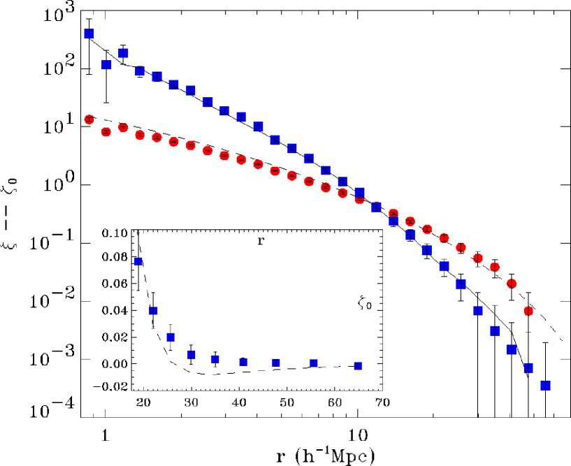
Figure 1: We display our measurements of the two- and three-point correlation functions $\xi$ (red solid circles) and $\zeta_{0}$ (blue solid squares) in the canonical M=$-21\sim-20$ volume limited sample. Error bars have been calculated from 22 2dF mocks. Solid line is our phenomenological model with parameters in Table 3, dashed lines are theoretical model with parameters in Table 5. Inset plotted on a linear scale for $\zeta_{0}$ on large scales.

3 Interpretation

3.1 Theoretical Framework

To interpret the clustering present in the 2dF, we use two models: theoretical model for large scales, and a phenomenological model for intermediate scales.

The theoretical model uses Eulerian perturbation theory (e.g., Bernardeau et al., 2002, and references therein) to calculate the real space dark matter three-point correlation function; specifically, we use the formulae in Szapudi (2005b).

Our bias model is motivated by the usual perturbative expansion $\delta_{g}=b\delta+b_{2}\delta/2+\ldots$ (Fry & Gaztanaga, 1993)

$$\xi_{g} =f_{2}b^{2}\left(\frac{\sigma_{8}}{0.9}\right)^{2}\xi$$ (6)

$$\zeta_{g,0} =\left(\frac{\sigma_{8}}{0.9}\right)^{4}\left[b^{3}f_{3}\zeta_{0}+b_{2}b^{2}f_{2}^{2}(\xi_{1}\xi_{2}+\xi_{2}\xi_{3}+\xi_{3}\xi_{1})_{0}\right],$$

where $b$ and $b_{2}$ are the linear and non-linear bias factors, $(...)_{0}$ denotes angular averaging, and $f_{2},\,f_{3}$ are redshift distortion enhancement factors (Kaiser, 1987; Hamilton, 1998)

$$f_{2} =\left(1+\frac{2}{3}f+\frac{1}{5}f^{2}\right)$$ (7)

$$f_{3} =\frac{5(2520+3360f+1260f^{2}+9f^{3}-14f^{4})}{98(15+10f+3f^{2})^{2}}\cdot\frac{7}{4}\ f_{2}^{2},$$

where $f=\Omega^{0}.6/b$. The third order $f_{3}$ is obtained by Pan & Szapudi (2005) through angle averaging perturbation theory results of Scoccimarro et al. (1999). Pan & Szapudi (2005) have shown this this is a good approximation to angle averaged three-point quantities with deviation at $5\%$ level.

Our phenomenological model is obtained by using directly our measured Virgo VLS redshift space two and three-point correlation functions in Equation 6 (with $f_{2}=f_{3}=1$ formally), with the exception that we still use the theory for $f_{2}^{2}(\xi_{1}\xi_{2}+\ldots)_{0}$ term.

3.2 Data Vectors

We intend to analyse the data in the above theoretical framework using maximum likelihood methods. When constructing a data vector from the measurements, we opt for not using ratio statistics of the sort $Q_{3}\simeq\zeta/\xi^{2}$ as it has been done in all previous studies, since our measurements include such large scales where $\xi$ becomes an extremely small number, possibly crosses zero. Our choice has the additional advantage that no ratio bias (e.g., Szapudi et al., 1999) appears, and our data have direct dependence on $\sigma_{8}$ which we will exploit.

We construct the data vector $(\xi,\zeta_{0})$ in an appropriate scale range, where the theoretical model is expected to be a good approximation (c.f. Table 2). Note that we excise redundant entries from the $\zeta_{0}(r_{1},r_{2})$ matrix, i.e. each pair of scales appears only once.

3.3 Covariance Matrix

Figure 2: This figure illustrates the structure of our covariance matrix, which follows from the set up of our data vectors, and the strong correlations among different bins of the two- and three-point correlation functions.

In order to perform a $\chi^{2}$ based maximum likelihood analysis, we estimate a covariance matrix from the 22 mock catalogs available. These have been extracted from the Virgo consortium Hubble volume simulation (Colberg et al., 2000). For details of generating catalogues and biasing see Cole et al. (1998). Volume limited subsamples were then created from each mock in exactly the same way as we do with the real data of 2dFGRS. Thus, for every volume limited subsample in Table 1 we have 22 measurements of the two- and three-point correlation functions.

We use the usual (biased) estimator for the covariance matrix,

$$\tilde{C}_{ij}=\frac{1}{N_{sim}}\sum_{I=1}^{N_{sim}}\Delta d^{I}_{i}\Delta d^{I}_{j}$$ (8)

where $\Delta d^{I}_{i}=d^{I}_{i}-\langle{d_{i}}\rangle$ is the $i$-th element of our data vector (containing $\xi$ and $\zeta_{0}$ and filtered according the previous subsection) from the $I$-th simulation; $N_{sim}=22$.

It can be shown, that a covariance matrix estimated by the above equation is necessarily singular if the number of simulations is less than the length of the data vectors (Szapudi & et al., 2005). More precisely, the rank of the matrix cannot be more than $N_{sim}$. In practice we have always found this rank to be $N_{sim}-1$ in several numerical experiments.

To calculate $\chi^{2}$ from a singular matrix, we use the singular value decomposition (SVD) method to create pseudo inverses (c.f. Gaztanaga & Scoccimarro, 2005). We have decomposed the $C$ matrix (the tilde denoting estimators is omitted from now on) as the multiple of three matrices

$$C=UWV^{T},$$ (9)

where $W$ is a diagonal matrix, and $U,V$ are orthogonal matrices; $V^{T}$ means transpose of $V$. The meaning of this decomposition is the kernel and image of the linear mapping $C$ (c.f. Press et al., 1992). Moreover, it is similar to an eigen-vector expansion, unique up to degenerate “eigenvalues”, the elements in W. To calculate $\chi^{2}$, we need $C^{-1}$ of our singular matrix. Since the inverse is formally $VW^{-1}U^{T}$, we can replace entries in $W^{-1}$ corresponding to small eigenvalues with $0$; this procedure is usually called constructing a pseudo-inverse.

We have found a marked drop in the eigenvalues beyond $N_{sim}-1$. We have checked that the corresponding columns of $U$ and $V$ are equal, i.e. they really are “eigenvectors” to all intents and purposes. It is meaningful to calculate $\chi^{2}$ with the above pseudo inverse, as long as the distribution of eigenvectors is Gaussian, as shown in Figure 3. In numerical simulations, we found that it is safe to keep about half of the eigenvectors, and for all measurements in this paper we used the top 10 eigenvalues and their corresponding entries in the $V$ matrix as eigenvectors. Our results are robust against this choice: have have checked using $8,9,10,11,12$ eigenvectors, and the results did not change significantly.

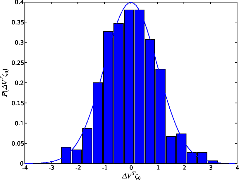
Figure 3: The distribution of modes corresponding to the large eigenvalues in $W$ in our 22 mock surveys. The mean have been subtracted, and each mode has been normalized to unit variance. The distribution appears to be consistent with Gaussian.

3.4 Maximum Likelihood Analysis

Using the data vector, and the pseudo inverse of the covariance matrix defined earlier, we can calculate $\chi^{2}=\Delta^{T}C^{-1}\Delta$, as well as likelihoods $p\propto\exp(-\chi^{2}/2)$ , where $\Delta=d-d_{th}(\sigma_{8},b,b_{2})$, $d_{th}$ is the theoretical model with explicit dependencies of the parameters. Note that in principle $C$ should also depend on the parameters, but we neglect that dependency. This is justified by the final results, which are not far from the mock surveys, and simplifies the calculation of likelihood enormously. To generalize this method, one would need to repeat the simulations and measurements for each set of parameters, as well as taking into account the determinant in the likelihood; this is clearly unfeasible at the moment.

4 Results

Table 2: Our filtering choices for the data vectors used in the analysis; the lower and upper cut offs are displayed in units of $\rm{h^{-1}Mpc}$. 3/P stands for 3 parameter maximum likelihood analysis based on our phenomenological model, 2/P and 2/T denotes 2 parameter fits to our phenomenological and theoretical models, respectively.

$M_{b_{J}}-5\log_{10}h$	3/P	2/P	2/T
-18 — -17	–	11.88 - 34.97	18.87 - 34.97
-19 — -18	4.04-34.97	10.18 - 34.97	18.87 - 47.61
-20 — -19	4.04-34.97	4.04 - 34.97	18.87 - 64.8
-21 — -20	5.49-34.97	11.88 - 34.97	18.87 - 64.8
-22 — -21	–	8.73 - 34.97	18.87 - 64.81

When applying the above described theoretical framework for the interpretation of our clustering measurements, special care needs to be taken about establishing scale ranges to be included in the data vectors for maximum likelihood analyses. On the one hand, we want to include as much data as possible to constrain parameters with the highest precision, on the other, if we include data points where the simple theoretical model is not a good approximation (for physical reasons and/or because of systematic errors), we might bias our results. Our considerations are detailed below.

For the theoretical model, a lower cut of $18\rm{h^{-1}Mpc}$ was used, where perturbation theory appears to be very accurate. In this case we use all scales up to $70\rm{h^{-1}Mpc}$ or the 1/4 of the characteristic scales of the slice, whichever smaller, to avoid severe edge effects.

For the phenomenological model we use our measurements from the VLS simulations as theory. Since we neglect the errors on these measurements, we use an upper cut of $35\rm{h^{-1}Mpc}$, above which the errors are non-negligible. The choice of the lower cut is more delicate. There is a complex interplay between accuracy of the simple bias and redshift distortion models we use with the emergence of discreteness effects. These finally determine the optimal cut in a fairly subtle way. The apparent complexity motivates an empirical approach: for the 2-parameter fits we perform maximum likelihood with a series of low cuts between $4\rm{h^{-1}Mpc}-14\rm{h^{-1}Mpc}$ for each magnitude limit, and finally choose the one with the lowest $\chi^{2}$. Fortunately we found that the two-parameter fits are robust against this choice, which nevertheless gives the tightest error bars possible.

For the three-parameter fit the empirical approach would be too expensive and we also want to maximize the range as much as possible to resolve the degeneracy between $\sigma_{8},b$. Therefore we use an absolute low cut of $4\rm{h^{-1}Mpc}$, below which non-linearities and complexity of the bias are expected to be strong, complemented with the condition, $\bar{n}r^{3}4\pi/3\geq 1$. This choice gives reasonable control over discreteness errors which could bias our fit giving a lower cut of $5.1\rm{h^{-1}Mpc}$ for the $-21\sim-20$ slice.

In our final choice we took the closest available bin from our logarithmic binning scheme to the above values. The scale ranges use in the fits are summarized in Table 2.

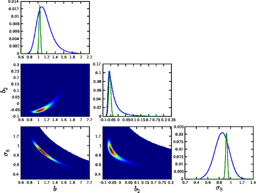
Figure 4: Three parameter likelihood contours for the magnitude slice $-21\sim-20$. The wider (blue) curves correspond to marginalized distributions, while the narrower (green) curves are a cut through the likelihood. The cut through the likelihood curve was normalized to the marginalized distribution at the maximum. Note that the actual value of the distribution is somewhat arbitrary, as it depends on the grid size. We also show two-dimensional marginalized likelihood contours to illustrate the correlations between the parameters.

4.1 Three-parameter Fits

Table 3: Three parameter fits to our two- and three-point clustering measurements. For each parameter, we present the maximum of the three-dimensional likelihood with error bars calculated form a $68$% of the marginalized distribution. In parentheses we display the maximum of the marginalized distribution.

$M_{b_{J}}-5\log_{10}h$	$\sigma_{8}$	$b$	$b_{2}$	$\chi^{2}$
-19 — -18	$1.07^{+0.09}_{-0.61}$ ( 0.80)	$0.81^{+0.53}_{-0.12}$ ( 0.89)	$-0.06^{+0.04}_{-0.03}$ (-0.06)	0.68
-20 — -19	$0.90^{+0.06}_{-0.28}$ ( 0.79)	$0.97^{+0.31}_{-0.14}$ ( 1.01)	$-0.04^{+0.06}_{-0.02}$ (-0.04)	3.11
-21 — -20	$0.93^{+0.04}_{-0.20}$ ( 0.85)	$1.04^{+0.23}_{-0.09}$ ( 1.08)	$-0.06^{+0.03}_{-0.01}$ (-0.06)	0.97

We calculated brute force 3 parameter grids with resolution $0.005$, and 2 parameter grids with resolution $0.001$. We checked the effects of grid resolution by repeating calculations with resolution $0.00025$ without any change in the results. While $\sigma_{8}$ and $b$ are quite degenerate along the line of $b\times\sigma_{8}=const.$, as expected, the inclusion of triangles in a large range of scales appears to break the degeneracy, at least for some of the samples. This is evidenced by the fact that a reasonable maximum has developed for the three volume limited samples in the mid-range. For those, we present our results in Table 3.

Error bars have been calculated from the marginalized curves using 68% thresholds. In the tables, the overall maximum is quoted first with error bars, while the maximum of the marginalized likelihood is presented in parentheses. The $\chi^{2}$ quoted is normalized to the degrees of freedom, which in this case is $10-3=7$.

The brightest and faintest magnitude limits do not support a three-parameter fits. Although they are statistically consistent with the three others presented, the large error bars due to the degeneracy of $\sigma_{8},b$ makes them meaningless. Similarly, the theoretical model does not support a stable three-parameter fit with either of the magnitude slices.

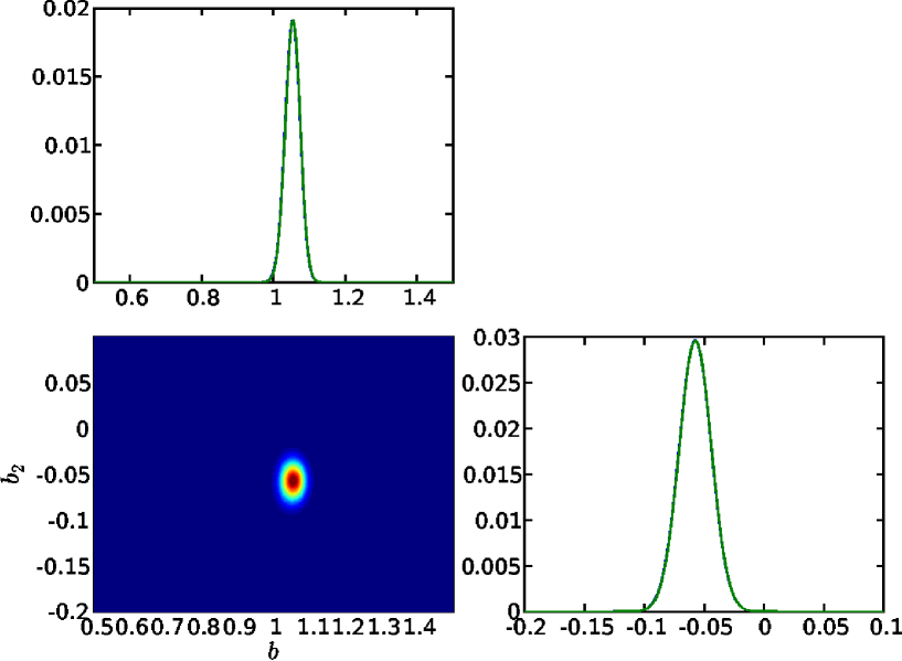
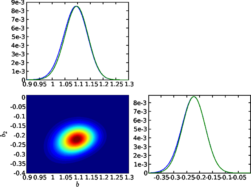
Figure 5: Two parameter likelihood contours for the $-21\sim-20$ slice. Both the phenomenological model (left) and the theoretical model (right) are displayed.

4.2 Two-parameter Fits

We also performed two-parameter fits using the bias parameters only. These approximately correspond to fitting $b\rightarrow b(\sigma_{8}/0.9)$. Fixing our reference $\sigma_{8}=0.9$ pins down the error bars which would otherwise explode due to the large degree of degeneracy. $\sigma_{8}=0.9$ is consistent with all our measurements, and these fits yield extremely precise values for the bias parameters. The effective degree of freedom is $10-2=8$.

Table 4: Two parameter fit based on the phenomenological model. Notation is the same as in Table 3

$M_{b_{J}}-5\log_{10}h$	$b$	$b_{2}$	$\chi^{2}$
-18 — -17	$0.807^{+0.128}_{-0.071}$ (0.833)	$-0.172^{+0.036}_{-0.027}$ (-0.164)	0.582
-19 — -18	$0.994^{+0.031}_{-0.036}$ (0.993)	$0.003^{+0.023}_{-0.023}$ (0.003)	0.343
-20 — -19	$0.969^{+0.027}_{-0.029}$ (0.968)	$-0.035^{+0.011}_{-0.012}$ (-0.035)	2.721
-21 — -20	$1.054^{+0.019}_{-0.021}$ (1.053)	$-0.057^{+0.012}_{-0.013}$ (-0.057)	0.372
-22 — -21	$1.273^{+0.095}_{-0.070}$ (1.274)	$0.006^{+0.086}_{-0.068}$ (0.010)	0.206

In the case of two-parameter fits, the theoretical model also supports stable likelihood surfaces and reasonable error bars, with the possible exception of the faintest magnitude limit, which we present for completeness only.

Table 5: Two parameter fit based on the theoretical model. Notation is the same as in Table 3

$M_{b_{J}}-5\log_{10}h$	$b$	$b_{2}$	$\chi^{2}$
-18 — -17	$0.484^{+0.063}_{-0.322}$ (0.358)	$-0.160^{+0.295}_{-0.334}$ (-0.151)	1.273
-19 — -18	$0.955^{+0.087}_{-0.134}$ (0.939)	$-0.252^{+0.132}_{-0.142}$ (-0.256)	1.248
-20 — -19	$0.945^{+0.071}_{-0.100}$ (0.935)	$0.185^{+0.053}_{-0.051}$ (0.184)	2.341
-21 — -20	$1.096^{+0.043}_{-0.049}$ (1.094)	$-0.222^{+0.044}_{-0.047}$ (-0.223)	0.747
-22 — -21	$1.385^{+0.080}_{-0.105}$ (1.375)	$-0.420^{+0.110}_{-0.110}$ (-0.425)	0.977

5 Summary and Discussions

We presented a measurement of the monopole of the three-point correlation function in the 2dFGRS. The new technology developed in Szapudi (2004); Pan & Szapudi (2005) enabled the estimation of the latter statistics in a wide range of scales from $1\rm{h^{-1}Mpc}-70\rm{h^{-1}Mpc}$. In the three-point function, up to $140\rm{h^{-1}Mpc}$ scales enter the measurements and the subsequent analysis. In addition, we measured the two-point correlation function.

To interpret these clustering statistics, we developed a novel maximum likelihood technique based on joint analysis of two- and three-point statistics. We estimated the joint correlation matrix from mock 2dF surveys. We seed the top 10 modes detected by an SVD of the joint correlation matrix to calculate a generalized $\chi^{2}$. The distribution of the modes is consistent with Gaussian, therefore we maximized the Gaussian likelihood with respect the the parameters of our theory. Our measurements are robust against keeping more or less eigen-modes, as well as against the scale range we use for the analysis. In Figure 6 we present the values for the bias parameter $b$ as a function of lower scale cut for both the phenomenological and theoretical models. Both models are fairly robust, as long as the $\chi^{2}\mathrel{\hbox{\hbox to0.0pt{\hbox{\lower 4.0pt\hbox{$\sim$}}\hss}\hbox{$<$}}}1$.

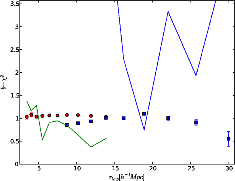
Figure 6: We illustrate the degree of robustness of our maximum likelihood fit by presenting the best fit bias parameters with error bars against the lower limit used in the fit (the upper limit was fixed to the value of Table 2). The (red) squares with error bars on the left (scales $4-14\rm{h^{-1}Mpc}$) show the phenomenological model, while on the right (blue) is the theoretical model (scales $9-25\rm{h^{-1}Mpc}$). The solid lines show the corresponding $\chi^{2}$’s of the fits. In general, as long as $\chi^{2}\mathrel{\hbox{\hbox to0.0pt{\hbox{\lower 4.0pt\hbox{$\sim$}}\hss}\hbox{$<$}}}1$, the fit is robust.

The significance of our three-parameter fit is that it yields a highly accurate measurement of $\sigma_{8}$ from large scale clustering alone. In particular, our estimate is independent of the cosmic microwave background (CMB). Yet, our value is in excellent agreement with those derived from Wilkinson Anisotropy probe (Spergel et al., 2003; Fosalba & Szapudi, 2004). $\sigma_{8}$ is still one of the most uncertain cosmological parameters, and our technique has a great potential to further improve the precision of its constraints. The virtually perfect agreement of $\sigma_{8}$ from CMB and large scale three-point level clustering is yet another one of the spectacular successes of the concordance model. In addition, our result is in excellent agreement with measurements based on SDSS two-point statistics and joint analysis with WMAP (Tegmark & et al., 2004; Pope & et al., 2004).

Our two parameter fits to the bias have extremely small error bars, they are likely to be systematics (both in the data and in the theory) limited. They can be considered as a measurement along the degeneracy line $b\sigma_{8}/0.9=$const., and can be directly compared with previous relative bias measurements from the 2dF. Figure 7 presents a comparison with Norberg et al. (2002), and shows excellent agreement.

We see no statistically significant evidence of scale dependency of the bias. Over the full scale range, from $4\rm{h^{-1}Mpc}-70\rm{h^{-1}Mpc}$, a constant bias model gave reasonable $\chi^{2}$’s. There is no significant trend between the measurements on intermediate, and large scales using the phenomenological and theoretical models respectively: the measured $b$’s are fully consistent with each other, and with Norberg et al. (2002). The only exception is the theoretical model for the faintest subsample, which also has fairly degenerate likelihood surfaces.

A possible check of systematics, although muddled by cosmic variance, is to estimate the bias in the NGP and SGP separately. Our phenomenological fits corroborate that of Verde et al. (2002), who find the SGP slightly more biased: our estimate is $b=1.025^{+0.040}_{-0.048}(1.022)$, and $b=1.097^{+0.020}_{-0.022}(1.096)$ for the NGP and SGP respectively. Nevertheless, the two samples are consistent at the 1-1.5$\sigma$ level, supporting the notion that the difference between them could be explained with cosmic variance alone.

The interpretation of our measurements in terms of Equations 6, 7 amounts to be some of the most comprehensive test of our picture of gravitational amplification with three point level large scale structure statistics. In particular, numerical experiments and theoretical calculations in the past tended to focus on a handful of triangular configurations, with preference for isoceles, and $1:2$ ratios. We have used all possible configurations (although monopole only) within our dynamic range and logarithmic binning system, and found a good fit to the data. The simplest explanation for this is that our basic picture of gravitational amplification is fundamentally correct. In particular, the results lend strong support to Gaussian initial conditions, and thus to inflation, even though we did not quantify this statement, since it was a prior in our model. Figure 1 shows the remarkable success of the theoretical and phenomenological models down to $1\rm{h^{-1}Mpc}$. The most natural interpretation of this is that bias is relatively simple, and that small scale redshift distortions largely cancel non-linear evolution in redshift space. There is a mild $1.5-2\sigma$ disagreement between the theoretical model and the data around $30-50\rm{h^{-1}Mpc}$. (c.f. inset of Figure 1). While this is not significant according to our measured overall $\chi^{2}$, it would be interesting to study this region with more accurate simulations, and higher order theoretical calculations.

On intermediate scales, we do not detect significant non-linear bias. On the other hand, the theoretical model on large scales detected non-linear bias at the $\simeq 2-4\sigma$ level. This could mean that either the theory is not accurate enough on the largest scales in accordance to the hint provided by the inset of Figure 1, and/or the largest scales might have some yet uncovered systematics, and/or there is significant non-linear bias. The latter possibility is somewhat unlikely since the intermediate scales do not display significant non-linear bias, and it would challenge the well established notion that bias should become simpler on larger scales. Nevertheless, Kayo et al. (2004) detected a surprizing complexity of non-linear bias with the three-point correlation function of the Sloan Digital Sky Survey. To decide between the possible explanations, one would need a highly accurate measurements of the three-point function reliable beyond $35\rm{h^{-1}Mpc}$. While this can and will be done in the future using the Hubble Volume (Colberg et al., 2000) or similar simulations, the present results do not allow distinguishing among the above possibilities without the risk of over-interpreting the data.

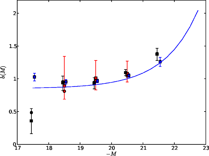
Figure 7: Comparison of our bias measurements with the relative bias measurements of Norberg et al. (2002). The solid line is $0.85+0.15(L/L^{*})$, where we normalized $L^{*}$ to be $M=-20.5$ magnitude. Red symbols in the middle with large error bars are the results of the three-parameter fit. Blue and black symbols show the phenomenological and theoretical fits respectively, and are shifted to left and right slightly for clarity. Squares and filled circles denote the maximum likelihood values in two-dimensions and in the marginalized distribution, respectively.

The technique we presented for constraining cosmological and bias parameters from joint likelihood analysis of two- and three-point statistics has enormous potential for further high precision cosmological applications. The constraining power of the present measurements is limited mainly by the theory. For one, only 22 simulations have been used to determine the covariance matrix. More accurate covariance matrix from a much larger number and realistic mocks could improve the statistical power of maximum likelihood estimation based on the same data. In addition, a more realistic model of bias and redshift distortions of the three point statistics, perhaps based on halo models (Takada & Jain, 2003; Fosalba et al., 2005), could enable the inclusion of all scales measured in the data vector for even tighter constraints.

The success of the three-parameter fits is remarkable, and it is a precursor of potentially even more accurate constraints, and perhaps fits to models with larger number of parameters. Perturbation theory can be thought of as a generalized bias with an anisotropic kernel (c.f. Matsubara, 1995). Since the standard bias model is isotropic, most information on separating bias from gravitational amplification should reside in higher order multipoles, such as dipole, and quadrupole. Measurements of these in the 2dF will be presented elsewhere. In particular, the higher order multipoles contain information on baryonic oscillations (Szapudi, 2004), which in turn might make it possible to constrain further cosmological parameters, such as baryon fraction, and dark energy.

Because of the small number of parameters we used so far, a brute force grid technique was feasible. If more parameters are fit, our technique lends itself naturally to Monte Carlo Markov Chain methods (e.g. Lewis & Bridle, 2002). Along the same lines, a useful and straightforward follow up to our investigation is joint likelihood analysis with CMB data. This and other generalizations will be presented elsewhere.

References

- Bernardeau et al. (2002) Bernardeau F., Colombi S., Gaztañaga E., Scoccimarro R., 2002, Phys. Rep., 367, 1
- Colberg et al. (2000) Colberg J. M., White S. D. M., Yoshida N., MacFarland T. J., Jenkins A., et al. 2000, MNRAS, 319, 209
- Cole et al. (1998) Cole S., Hatton S., Weinberg D. H., Frenk C. S., 1998, MNRAS, 300, 945
- Cole et al. (2005) Cole S., Percival W. J., Peacock J. A., Norberg P., et al. 2005, ArXiv Astrophysics e-prints, astro-ph/0501174
- Colless et al. (2001) Colless M., Dalton G., Maddox S., Sutherland W., Norberg P., et al. 2001, MNRAS, 328, 1039
- Colless et al. (2003) Colless M., Peterson B. A., Jackson C., Peacock J. A., Cole S., et al. 2003, ArXiv Astrophysics e-prints,astro-ph/0306581
- Croton et al. (2004) Croton D. J., Gaztañaga E., Baugh C. M., Norberg P., Colless M., et al. 2004, MNRAS, 352, 1232
- Feldman et al. (2001) Feldman H. A., Frieman J. A., Fry J. N., Scoccimarro R., 2001, Physical Review Letters, 86, 1434
- Fosalba et al. (2005) Fosalba P., Pan J., Szapudi I., 2005, submitted to ApJ, astro-ph/0504305
- Fosalba & Szapudi (2004) Fosalba P., Szapudi I., 2004, ApJ, 617, L95
- Fry (1994) Fry J. N., 1994, Physical Review Letters, 73, 215
- Fry & Gaztanaga (1993) Fry J. N., Gaztanaga E., 1993, ApJ, 413, 447
- Gaztanaga & Scoccimarro (2005) Gaztanaga E., Scoccimarro R., 2005, ArXiv Astrophysics e-prints
- Hamilton (1998) Hamilton A. J. S., 1998, in ASSL Vol. 231: The Evolving Universe Linear Redshift Distortions: a Review. pp 185–+
- Hawkins et al. (2003) Hawkins E., Maddox S., Cole S., Lahav O., et al. 2003, MNRAS, 346, 78
- Jing & Börner (2004) Jing Y. P., Börner G., 2004, ApJ, 607, 140
- Kaiser (1984) Kaiser N., 1984, ApJ, 284, L9
- Kaiser (1987) Kaiser N., 1987, MNRAS, 227, 1
- Kayo et al. (2004) Kayo I., Suto Y., Nichol R. C., Pan J., Szapudi I., et al. 2004, PASJ, 56, 415
- Landy & Szalay (1993) Landy S. D., Szalay A. S., 1993, ApJ, 412, 64
- Lewis & Bridle (2002) Lewis A., Bridle S., 2002, Phys. Rev. D, 66, 103511
- Macfarland et al. (1998) Macfarland T., Couchman H. M. P., Pearce F. R., Pichlmeier J., 1998, New Astronomy, 3, 687
- Matarrese et al. (1997) Matarrese S., Verde L., Heavens A. F., 1997, MNRAS, 290, 651
- Matsubara (1995) Matsubara T., 1995, ApJS, 101, 1
- Norberg et al. (2001) Norberg P., Baugh C. M., Hawkins E., Maddox S., et al. 2001, MNRAS, 328, 64
- Norberg et al. (2002) Norberg P., Cole S., Baugh C. M., Frenk C. S., Baldry I., et al. 2002, MNRAS, 336, 907
- Pan & Szapudi (2005) Pan J., Szapudi I., 2005, MNRAS, in press. astro-ph/0405590
- Percival et al. (2001) Percival W. J., Baugh C. M., Bland-Hawthorn J., Bridges T., et al. 2001, MNRAS, 327, 1297
- Pope & et al. (2004) Pope A. C., et al. 2004, ApJ, 607, 655
- Press et al. (1992) Press W. H., Teukolsky S. A., Vetterling W. T., Flannery B. P., 1992, Numerical recipes in C. The art of scientific computing. Cambridge: University Press, —c1992, 2nd ed.
- Scoccimarro (2000) Scoccimarro R., 2000, ApJ, 544, 597
- Scoccimarro et al. (1999) Scoccimarro R., Couchman H. M. P., Frieman J. A., 1999, ApJ, 517, 531
- Spergel et al. (2003) Spergel D. N., Verde L., Peiris H. V., Komatsu E., Nolta M. R., et al. 2003, ApJS, 148, 175
- Szapudi (1998) Szapudi I., 1998, ApJ, 497, 16
- Szapudi (2004) Szapudi I., 2004, ApJ, 605, L89
- Szapudi (2005a) Szapudi I., 2005a, in. prep.
- Szapudi (2005b) Szapudi I., 2005b, in press, astro-ph/505391
- Szapudi & Colombi (1996) Szapudi I., Colombi S., 1996, ApJ, 470, 131
- Szapudi et al. (1999) Szapudi I., Colombi S., Bernardeau F., 1999, MNRAS, 310, 428
- Szapudi & et al. (2005) Szapudi I., et al. 2005, in. prep.
- Szapudi & Szalay (1998) Szapudi S., Szalay A. S., 1998, ApJ, 494, L41
- Takada & Jain (2003) Takada M., Jain B., 2003, MNRAS, 340, 580
- Tegmark & et al. (2004) Tegmark M., et al. 2004, Phys. Rev. D, 69, 103501
- Verde et al. (1998) Verde L., Heavens A. F., Matarrese S., Moscardini L., 1998, MNRAS, 300, 747
- Verde et al. (2002) Verde L., Heavens A. F., Percival W. J., Matarrese S., et al. 2002, MNRAS, 335, 432
- Wang et al. (2004) Wang Y., Yang X., Mo H. J., van den Bosch F. C., Chu Y., 2004, MNRAS, 353, 287