A universal velocity distribution of relaxed collisionless structures

Abstract

Several general trends have been identified for equilibrated, self-gravitating collisionless systems, such as density or anisotropy profiles. These are integrated quantities which naturally depend on the underlying velocity distribution function (VDF) of the system. We study this VDF through a set of numerical simulations, which allow us to extract both the radial and the tangential VDF. We find that the shape of the VDF is universal, in the sense that it depends only on two things namely the dispersion (radial or tangential) and the local slope of the density. Both the radial and the tangential VDF’s are universal for a collection of simulations, including controlled collisions with very different initial conditions, radial infall simulation, and structures formed in cosmological simulations.

1 Introduction

The last few years have shown remarkable progress in the understanding of pure dark matter structures. This has been provided initially by numerical simulations which have observed general trends in the behaviour of the radial density profile of equilibrated dark matter structures from cosmological simulations, which roughly follow an NFW profile [1, 2], see [3] for references. General trends in the radial dependence of the velocity anisotropy has also been suggested [4, 5]. More recently have more complex relations been identified, which even hold for systems which do not follow the most simple radial behaviour in density. These relations are first that the phase-space density, $\rho/\sigma^{3}$, is a power-law in radius [6], and second that there is a linear relationship between the density slope and the anisotropy [7].

All of these are integrated quantities, and still very little is known about the underlying velocity distribution function (VDF) of real collisionless systems. We will here initiate such a study by performing a set of different simulations of purely collisionless systems. We will then extract the VDF and split this into the radial part and the tangential part for numerous bins in potential energy. This will allow us to more fully appreciate the complicated structure of the VDF. We will show that within the structures which have been perturbed strongly and subsequently allowed to relax, both the radial and the tangential VDF’s have a universal shape. This shape is given only as function of the velocity dispersion and the local density slope.

2 Head-on collisions

The first controlled simulation is the head-on collision between two initially isotropic NFW structures. For the construction of the initial structures, we use the Eddington method as described in [8], which imposes an exponential cut-off in the very outer region. We create an initial NFW structure with zero anisotropy containing 1 million particles. The parameters are chosen corresponding to a total mass of $10^{12}$ solar masses (concentration of 10), and half of the particles are within 160 kpc. The structure is in equilibrium in the sense that when evolving such a structure in isolation its global properties remain unchanged.

We now place two such structures very far apart with 2000 kpc between the centres, which is well beyond the virial radius. Using a softening of 0.2 kpc, we now let these two structures collide head-on with an initial relative velocity of 100 km/sec towards each. After several crossings the resulting blob relaxes into a prolate structure. We run all simulations until there is no further time variation in the radial dependence of the anisotropy and density. We check that there is no (local) rotation. We run this simulation for 150 Gyrs, which means that a very large part of the resulting structure is fully equilibrated.

We now take the resulting structure (now containing 2 million particles, in a prolate shape) and collide 2 copies together, again with their centres separated by 2000 kpc, and with initial relative velocity of 100 km/sec. We now use softening of 1 kpc. The resulting structure is even more prolate when observed in density contours, and we evolve this for another 150 Gyr.

All simulations were carried out using PKDGRAV, a multi-stepping, parallel code [9], which uses spline kernel softening and multi-stepping based on the local acceleration of particles. The simulations were performed on the zBox at Zurich University.

In order to analyze the resulting structure we divide it into bins in potential energy, linearly distributed from the softening length to beyond the region which is fully equilibrated. For the analysis and figures presented in this paper, we always only include a region outside 3 times the softening. We center the structure on the center of potential (using potential as weight-function instead of mass as done for center of mass). Most other analyses are centering on either the center of mass, or on the most bound particle, but the difference is very small. We calculate the local density for each particle from its nearest 32 neighbours, and we average the density for all the particles in the potential bin. Similarly, each particle has a radius from the center of potential, and we can average this over all the particles in the potential bin. The resulting density profile, $\langle\rho\rangle$ as a function of $\langle r\rangle$, is very similar to an NFW profile (see figure 1).

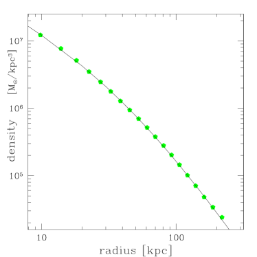
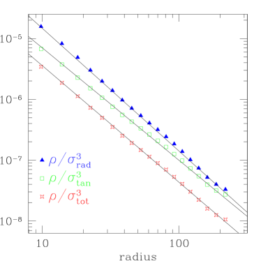
Figure 1: Left panel: Resulting density profile of a repeated head-on collision between two initially isotropic NFW structures. The thin black line is of the NFW shape. Right panel: Resulting phase-space density profile of a repeated head-on collision between two initially isotropic NFW structures. The thin black lines are just power-laws in radius, with slopes $-2.02$ (radial), $-1.85$ (tangential), and $-1.92$ (total).

One can also calculate velocity dispersions for each potential bin of the structure. We split the velocities into radial and tangential, and on figure 1 we present the phase-space density, $\rho/\sigma^{3}$, as a function of radius. The $\sigma$ can be either the radial, tangential or total. The relationship between phase-space density and radius has been considered several times [6, 10, 11, 12, 13] and seems to be well established. Using the Jeans equation together with the fact that phase-space density is a power-law in radius allows one to find the density slope in the central region numerically [6], and even analytically for power-law densities [14]. Recently a much refined study [10] using both the phase-space density being a power-law in radius and also the linear relationship between density slope and anisotropy, showed that one can solve the Jeans equations analytically and extract the radial dependence of density, anisotropy, mass etc. This analysis was made using $\sigma_{\rm rad}$. Whereas we here confirm that the phase-space density roughly follows a power-law in radius, then it is not clear which of the dispersions leads to a better fit to a power-law (see figure 1). Given the fact that the anisotropy changes as function of radius, then if one of the phase-space densitities (e.g. using $\sigma_{rad}$) is a power-law, then the other (e.g. using $\sigma_{tot}$) must have slightly s-shaped residuals.

For each bin we can also define the radial derivative of the density (the density slope)

$$\alpha\equiv\frac{d{\rm ln}\langle\rho\rangle}{d{\rm ln}\langle r\rangle}\,,$$ (1)

and we can extract the radial velocity distribution function (VDF) for each potential bin. We present the radial VDF for bins with $\alpha\approx-2.6,-2$ and $-1.1$ in the left panel of figure 2. The red (open) stars are from a bin in the region with shallow density slope ($\alpha\approx-1.1$), the green (open) squares are from an intermediate bin (slope close to $-2$), and the blue (filled) triangles are from a bin in the outer region (slope close to $-2.6$). There seems to be a clear trend, namely that the VDF from bins in the inner region have longer high energy tails than VDF’s from bins in the outer region. On the same figure have we overplotted 3 black (solid) lines, which have the shape

$$f_{r}(v)=\left(1-(1-q)\,\left(\frac{v}{\kappa_{1}\,\sigma_{\rm rad}}\right)^{2}\right)^{\frac{q}{1-q}}\,,$$ (2)

where $q$ and $\kappa_{1}$ are free parameters. This is of the Tsallis form [15], and depends on the entropic index $q$. This form reduces to the Gaussian shape $f(v)\sim{\rm exp}(-(v/v_{0})^{2})$ when $q=1$. This functional form is chosen partly for simplicity (and because it includes the classical exponential), and partly because some simple structures are know to have VDF’s of exactly this form [16, 17]. The corresponding $q$’s of these 3 lines in figure 2 are $0.75,0.81,1.08$, showing that the bin in the region with more shallow density slopes (with $q=1.08$) has a longer high energy tail than a Gaussian. In particular do we see that the resulting VDF’s do not have the shape of Gaussians with a cut-off at the escape velocity.

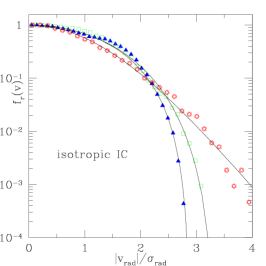
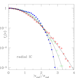
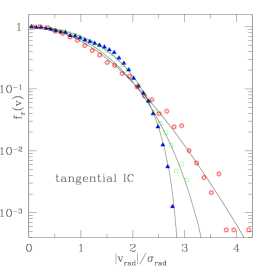
Figure 2: The radial VDF for 3 potential bins in the simulation of repeated headon collisions between NFW structures with very different initial conditions. The potential bins are chosen near density slope of $\alpha\approx-1.1$ (open red stars), $\alpha\approx-2$ (open green squares) and $\alpha\approx-2.6$ (filled blue triangles). The thin (solid) lines are of the shape given by eq. (2), using $q$’s of $0.75,0.81$ and $1.08$ (fig a); $q=0.79,0.91$ and $1.05$ (fig b); and $q=0.75,0.89$ and $1.045$. The similarity between these figures is striking.

The shape of eq. (2) provides a reasonable fit to all the energy range only for the most shallow profile, namely in the spatial region where the velocity dispersion is isotropic. In the regions with steeper density profile does the shape of eq. (2) only provide a fit in the high energy region of the VDF, and in order to fully fit the radial VDF in the low energy region must one consider a more general shape. Detailed look at the figures in fig. 2 reveals that the general radial VDF may be better fit with a more flat-topped (larger $q$) in the low energy region, and with a (small) $q$ as described above for the high energy region, however we will not pursue this issue further here.

It is worth commenting briefly on the definition of radial and tangential used in this paper. We are splitting the equilibrated structure in potential bins, which is because the energy of each particle is composed of potential and kinetic energy. Since we wish to extract the VDF’s, then we must consider potential bins and not radial bins, however, the potential bins are virtually spherical in the outer region, and there is only a small effect in the central region. Now, we define ”radial” strictly with respect to a spherical symmetry. Clearly the splitting between radial and tangential will depend somewhat on the actual shape of the structure considered: if the structure is very elongated, then the concept of ”radial” must be with respect to the shape of this structure. One can extract the shape from either density contours or from the potential energy contours, and the shape will be different (density contours are much more triaxial), and hence the definition of ”radial” depends on which kind of shape one is referring to. We will in this paper, for simplicity, ignore this complication, and simply extract the radial with respect to spherical symmetry. We hope to discuss this issue in full in a future analysis.

2.1 Dependence on initial conditions?

To address the question of how strongly the VDF’s from the head-on collisions described above depend on the initial conditions, we now consider 2 simulations each with two steps. i) First we create a spherical isotropic NFW structure with 1 million particles as described above. We take each individual particle in this structure and put its total velocity along the radial direction, maintaining the sign with respect to inwards or outwards from the halo centre. We keep the energy of each particle fixed. This structure is thus strongly radially anisotropic. ii) Now we take two such radially anisotropic structures and place their centres 2000 kpc apart (well outside the virial radius) with relative velocity of 100 km/sec towards each other. We use softening of 1 kpc for these tests. Before the centres of the two structures collide the radial motion of the particles behaves almost like a radial infall simulation, and strong scattering of the particles is observed. The 2 individual structures pick random orientations in space as they become triaxial [18]; their orientations are completely erased after the two structures collide head-on. We let the structure equilibrate. We take two copies of the resulting structure and collide these head-on, again with 100 km/sec. The final equilibrated region contains approximately 2.5 million particles (of the total of 4 million particles).

The resulting VDF’s extracted in potential bins near density slopes of $-2.3,-2,-1.2$ are shown in the central panel of figure 2, and the black (solid) lines are again of the shape of eq. (2), with $q$’s of $0.79,0.91$ and $1.05$.

Second, we run a simulation identical to the one just described, except that we place each individual particle in the initial structures on tangential orbits, without changing the energy of the individual particles. This initial condition thus corresponds to strongly tangential motion. When letting this structure equilibrate in isolation it settles down with a tangential anisotropy of $\beta\sim-2$. Again, two such structures are collided head-on. We again take two copies of the resulting structure and collide these headon. The resulting VDF’s are shown in the right panel of figure 2, where the bins were chosen to be near density slope of $-2.6,-2$ and $-1.15$, and the black (solid) lines are of the shape eq. (2), with $q$’s of $0.75,0.89$ and $1.045$. One should keep in mind, that this last structure was created with zero radial velocity, and hence the radial VDF was created while perturbing the structure and letting it relax.

It is clear from the figures above, that the simple shape of eq. (2) provides a reasonable fit to the tails of the radial VDF’s. Furthermore, there seems to be a general trend in the connection between density slope and the best fitting $q$, which is shown in figure 3 as blue (solid) triangles.

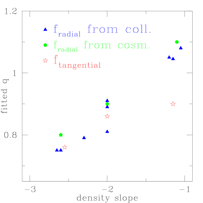
Figure 3: The $q$’s which best fit the high energy tail of the radial VDF’s (blue triangles) as a function of the density slope. The green (filled) pentagons are fitted from the radial VDF’s of a combination of cosmological simulations and a radial collapse simulation. The red (open) stars are the $q$’s which best fit the high energy tail of the 2 dimensional tangential VDF. There is a general trend, namely that more shallow slopes are better fit with higher q.

Such a trend with shallower density slope implying larger $q$’s was suggested from simplified theoretical considerations [17]. It is interesting to note that ref. [19] found that the radial VDF of the inner-most bin is fit with a Gaussian $q=1$, and the intermediate bins can be fitted with $q=0.65$, in reasonable agreement with our findings.

Finally we consider simulated cosmological $\Lambda$CDM haloes that form in a standard expanding hierarchical universe, and we analyse these haloes in the same way as above. We consider two relaxed halos, each with approximately 1/2 million particles in the equilibrated region. These are the two binary haloes taken from the Local Group simulation of [20]. One of these haloes is strongly oblate, the other strongly prolate in density contours. We also perform a radial infall simulation with 1 million particles, and analyse the resulting structure as described above. We first present the density and phase-space density of the radial infall simulation as functions of radius (in simulation units) in figure 4, from which it appears that using the total dispersion leads to a slightly better fit to a power-law in radius, since the residuals from a power-law is slightly s-shaped when using $\sigma_{rad}$ instead.

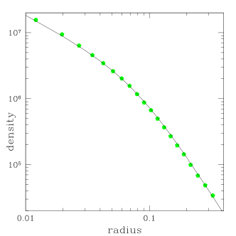
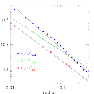
Figure 4: The density and phase-space density as functions of radius for the radial collapse model. The black line in the left panel is of the NFW shape. Right panel: The symbols are when using different dispersions (radial, tangential, total), and it appears that using the total dispersion provides a slightly better fit to a power-law in radius. The solid (thin) black lines are power-laws in radius, using powers of $-1.9$ (radial), $1.4$ (tangential), and $-1.6$ (total).

For these 3 simulations we extract the VDF’s in potential bins, and we present these 3 simulations together in the left column of figure 5, where we are plotting the radial VDF for bins with density slope near $-1.1,-2$ and $-2.6$ respectively. Also in these figures do we plot black (solid) lines of the form in eq. (2), using $q$’s of $1.1,0.9$ and $0.8$ respectively. A potential bin near density slope of $-2.6$ has much larger scatter since this region is not fully mixed in the cosmological runs. We present the corresponding $\alpha$’s and $q$’s as green (filled) pentagons in figure 3, and we find good agreement with the results from the controlled collisions.

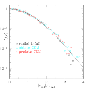
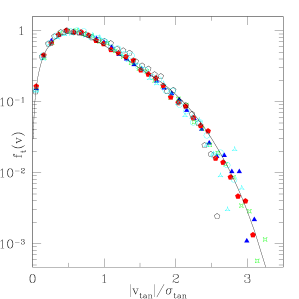
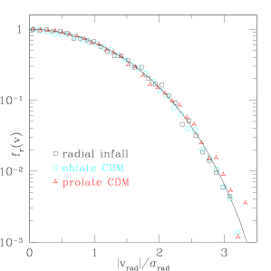
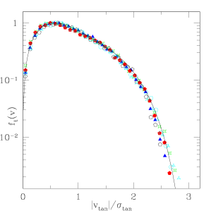
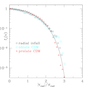
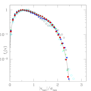
Figure 5: Left column: The radial VDF’s from a cosmological simulation (blue circles and red triangles) and a radial infall simulation (black squares). Row 1: The potential bins were chosen near density slope of $\alpha=-1.1$, and the black (solid) line is of the shape in eq. (2), using $q=1.1$. Row 2: $\alpha=-2$, $q=0.9$. Row 3: $\alpha=-2.6$, $q=0.8$. Right column: The tangential VDF’s from all the simulations discussed above. The black (solid) line has two parts (separated at $v_{\rm tan}=1.6\,\sigma_{\rm tan}$), each fitted with the shape given in eq. (3), where the low energy part uses $q=5/3$, and the outer region (high energy part) has a free $q$. Row 1: using a potential bin near the density slope of $\alpha=-1.1$, and the black (solid) line uses $q=0.9$ in the high energy part. Row 2: $\alpha=-2$, $q=0.86$. Row 3: $\alpha=-2.6$, $q=0.76$.

3 Tangential VDF

In order to discuss the shape of the tangential VDF we now present the tangential VDF in 3 bins from each of the simulations described above. These are the same bins as discussed for the radial VDF, namely one bin in the outer region (near $\alpha=-2.6$), a bin near an intermediate slope (near $\alpha=-2$), and a bin near a shallow density slope (near $\alpha=-1.1$).

The first impression from the right column of figure 5 is that indeed all the tangential VDF’s look very similar for these different simulations: the simulations with 4 million particles which have been run for a very long time (red, blue and green symbols) lie very close to each other, and the scatter in figure 5 is from the low resolution structures from the cosmological simulation (each with about 1/2 million particles) and the radial infall simulation (with 1 million particles). This scatter is most visible for the bin near a shallow profile (top panel) where there are relatively few particles.

One should keep in mind that the initial conditions for two of these simulations were with all the particles on completely radial orbits, and therefore the tangential VDF’s appear purely as a result of the structure being perturbed and setteling down in a stable configuration.

When comparing figures 5 one sees another trend, namely that the high energy tail of the VDF becomes longer for more shallow density profile. This was exactly what we noticed for the radial VDF above.

These are the 2-dimensional tangential VDF’s, and for a classical gas they would have had the shape $f_{t}\sim v\,{\rm exp}(-v^{2}/v_{0}^{2})$, where $v_{0}$ is some normalizing velocity. We see clearly from the figures that they all have a rather characteristic break, somewhere near $v_{\rm tan}=2\,\sigma_{\rm tan}$, and hence a Gaussian will give a very poor fit.

We are interested in making a phenomenological fit to the shape of these tangential VDF, and it is natural to consider the 2-dimensional generalization of eq. (2), namely

$$f_{t}(v)=v\,\left(1-(1-q)\,\left(\frac{v}{\kappa_{2}\,\sigma_{\rm rad}}\right)^{2}\right)^{\frac{q}{1-q}}\,,$$ (3)

however, given the break near $v_{\rm tan}=2\,\sigma_{\rm tan}$ this is clearly not sufficient. We will therefore fit with two such shapes, one in the small velocity region, and another in the high velocity region. It was argued in [7] that the tangential VDF’s could have the shape of eq. (3) with $q=5/3$, and one sees immedeately that the small velocity region is very well fit with exactly this shape for all the bins in potential. We pick the position $v_{\rm tan}=1.6\,\sigma_{\rm tan}$ as the transition velocity for all figures, and fit the high energy region with the shape of eq. (3), but with $q$ a free parameter. The combined fit is shown as black (solid) lines in the 3 figures, and these provide a very good fit to the full VDF’s. We are using $q$’s of $0.76,0.86$ and $0.9$ (larger $q$ corresponds to more shallow density profile). These results for the high energy tail of the tangential VDF’s are also shown in figure 3 as red (open) stars. Again there is a general trend showing that more shallow density profiles give tangential VDF’s which have power-law tails given by larger $q$’s.

4 Full VDF

Having identified that both the radial and the tangential distribution functions have the same universal shapes for different simulations, for potential bins which are at the same value of the density slope, we can now also plot the full (3 dimensional) VDF. Also cosmological simulations have considered the full VDF and found that a Gaussian in general does not give a good fit to the VDF [20, 21].

A comment on the uniqueness of the connection between the VDF’s and the density is in order at this point. The density is simply given as an integral over the full VDF, $\rho=\int f\,d^{3}v$, however, this is completely independent of the anisotropy. If the anisotropy is zero, then this equation can be inverted for spherical systems (by the Eddington method) to give the VDF as a function of the density profile. This inversion gives a unique VDF. However, for an anisotropic and non-spherical system this inversion is almost certainly not unique, and it is therefore not obvious that the VDF should be universal between these different simulations. On a more philosophical note, one should keep in mind that the individual particles are gravitationally scattered off each other while the structures are forming: the individual particles only feel the local particles and the local change of density and potential. It is therefore the VDF’s which are truely universal. The integrated quantities, namely density and anisotropy, are universal because of the universality of the VDF’s. If we are ever going to truely understand the universality of density and anistropy, then we should take a step back and understand the universality of the VDF’s.

Instead of plotting for all the simulations, we will only show the full VDF for one, namely the repeated head-on collision between initially isotropic NFW structures. This is shown in figure 6, where the potential bins are chosen near density slope of $\alpha\approx-1.1$ (open red circles), $\alpha\approx-2$ (open green squares) and $\alpha\approx-2.6$ (filled blue triangles).

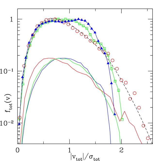
Figure 6: The total 3-dimensional VDF for 3 potential bins in the simulation of a repeated headon collision between initially isotropic NFW structures. The potential bins are chosen near density slope of $\alpha\approx-1.1$ (open red circles), $\alpha\approx-2$ (open green squares) and $\alpha\approx-2.6$ (filled blue triangles). The solid lines which are shifted downwards for visibility are from the isotropic NFW structure, and do not exhibit the double-hump.

In the spatially central region with shallow density profile there is zero anisotropy, and the full VDF can again be reasonably fitted by two functions of the shape $f_{\rm tot}=v^{2}\,f_{r}$. This is shown with the dashed (black) line going through the red circles (using different $q$’s in the high and low energy region, $q_{1}\approx 1.3,q_{2}\approx 1$). In the spatial regions with non-zero anisotropy the full VDF looks much more complicated, in particular, in regions with large anisotropy is develops a double-hump shape (see blue filled triangles in figure 6). For comparison we show the corresponding full VDF from the initial conditions of a stable NFW structure with zero anisotropy as solid lines shifted downwards for visibility (regions corresponding to the same density slope as for the repeated head-on collision). These initial conditions clearly do not have the double-hump, since they are isotropic.

5 Conclusions

We have identified a universality of the velocity distribution function (VDF) of equilibrated structures of collisionless, selfgravitating particles through a set of controlled numerical experiments. We find that the radial and tangential VDF are universal in the sense that they depend only on the dispersion (radial or tangential) and the local slope of the density. This universality of the VDF is non-trivial, since the final structures are not spherical and isotropic.

Our simulations include controlled collision experiments between structures which are initially isotropic as well as highly anisotropic, radial infall collapse, and structures formed in cosmological simulations.

The high energy tail of the radial VDF is well approximated by the shape given in eq. (2), however, for regions with non-zero anisotropy (steep density slopes) there are corrections in the low-energy part of the VDF.

The tangential VDF is well described by a combination of two functions of the shape of eq. (3), where the low-energy part has $q=5/3$, and the high-energy part has a $q$ similar to the one describing the radial VDF.

Whereas the general trend, namely that steeper density slope implies small $q$, is in agreement with theoretical expectations, then the actual shape of the VDF’s is not understood yet. Our numerical results may hopefully inspire further theoretical understanding of the VDF of collisionless particles.

References

References

- [1] Navarro, J. F., Frenk C. S. & White, S. D. M. 1996, ApJ, 462, 563
- [2] Moore, B., Governato, F., Quinn, T., Stadel, J. & Lake G. 1998, ApJ, 499, 5
- [3] Diemand, J., Moore, B. & Stadel, J. 2004, 353, 624
- [4] Cole S. & Lacey C. 1996, MRNAS, 281, 716
- [5] Carlberg R. G. 1997, ApJ, 485, L13
- [6] Taylor, J. E. & Navarro, J. F. 2001, ApJ, 563, 483
- [7] Hansen, S. H. & Moore, B. 2004, arXiv:astro-ph/0411473
- [8] Kazantzidis S., Magorrian J. & Moore B., 2004, ApJ, 601, 37
- [9] Stadel J. 2001, PhD thesis, University of Washington
- [10] Dehnen W. & McLaughlin, D. 2005, arXiv:astro-ph/0506528
- [11] Rasia, E., Tormen, G. & Moscardini, L. 2004, MNRAS, 351, 237
- [12] Ascasibar, Y., Yepes, G., Gottlöber, S. & Müller, V. 2004, MNRAS, 352, 1109
- [13] Austin, C. G. et al. 2005, arXiv:astro-ph/0506571.
- [14] Hansen, S. H 2004, MNRAS, 352, L41
- [15] Tsallis, C. 1988, J. Stat. Phys., 52, 479
- [16] Plastino, A. R. & Plastino, A. 1993, PLA, 173, 384
- [17] Hansen, S. H., Egli, D., Hollenstein, L. & Salzmann, C. 2005, New Astron., 10, 379
- [18] Merritt, D. 1985, MNRAS, 217, 787
- [19] Wojtak, R. et al. , 2005, MNRAS (in press), arXiv:astro-ph/0503391.
- [20] Moore, B. et al. 2001, PRD, 64, 063508
- [21] Diemand, J., Moore, B. & Stadel, J. 2004, MNRAS, 352, 535