Subaru Super Deep Field with Adaptive Optics I.
Observations and First Implications

Abstract

We present a deep $K^{\prime}$-band (2.12$\mu$m) imaging of 1′ $\times$ 1′ Subaru Super Deep Field (SSDF) taken with the Subaru adaptive optics (AO) system. Total integration time of 26.8 hours results in the limiting magnitude of $K^{\prime}\sim 24.7$ (5$\sigma$, 0$\farcs$2 aperture) for point sources and $K^{\prime}\sim 23.5$ (5$\sigma$, 0$\farcs$6 aperture) for galaxies, which is the deepest limit ever achieved in the $K^{\prime}$ band. The average stellar FWHM of the co-added image is 0$\farcs$18. Based on the photometric measurements of detected galaxies, we obtained the differential galaxy number counts, for the first time, down to $K^{\prime}\sim 25$, which is more than 0.5 mag deeper than the previous data. We found that the number count slope $d\log N/dm$ is about 0.15 at $22<K^{\prime}<25$, which is flatter than the previous data. Therefore, detected galaxies in the SSDF have only negligible contribution to the near-infrared extragalactic background light (EBL), and the discrepancy claimed so far between the diffuse EBL measurements and the estimated EBL from galaxy count integration has become more serious . The size distribution of detected galaxies was obtained down to the area size of less than 0.1 arcsec², which is less than a half of the previous data in the $K^{\prime}$ band. We compared the observed size-magnitude relation with a simple pure luminosity evolution model allowing for intrinsic size evolution, and found that a model with no size evolution gives the best fit to the data. It implies that the surface brightness of galaxies at high redshift is not much different from that expected from the size-luminosity relation of present-day galaxies.

1. Introduction

The process of galaxy formation and evolution is one of the most important unsolved problems in astrophysics. Deep imaging of blank field is a vital method for studying the properties of galaxies in the distant universe (Yoshii & Takahara, 1988). The Hubble Deep Field (HDF) taken by the Hubble Space Telescope (HST) had revealed deep images of the universe at optical wavelengths (Williams et al., 1996, 2000; Gardner et al., 2000), and provided us with valuable information of the distant universe. However, for high-redshift galaxies at $z>1$, the rest-frame optical light, that exhibits the fundamental structure of stellar component in galaxies, shifts into the infrared (e.g. Sheth et al. 2003). Therefore, the near infrared (NIR) deep imaging becomes important to study the formation and evolution of galaxies at high-redshifts. Moreover, the uncertainties due to the evolution of galaxies and extinction by interstellar dust are less significant in the longer wavelength. Thus, deep imaging in the $K$ (2.2$\mu$m) band, that is the longest wavelength at which the high-sensitive observations can be carried out from the ground, is essential to study the fundamental properties of high-redshift galaxies.

A number of $K$-band imaging surveys were carried out using ground-based large telescopes with different spatial coverages and limiting magnitudes (e.g. Gardner et al. 1993, 1996; Glazebrook et al. 1994; Mcleod et al. 1995; Djorgovski et al. 1995; Huang et al. 1997; Moustakas et al. 1997; Szokoly et al. 1998; Minezaki et al. 1998a; Bershady et al. 1998; Saracco et al. 1999; Väisänen et al. 2000; Martini 2001; Maihara et al. 2001; Baker et al. 2003; Cristóbal-Hornillos et al. 2003; Labbe et al. 2003). Among these surveys, the deep $K^{\prime}$ (2.12$\mu$m) imaging of the Subaru Deep Field (SDF, Maihara et al., 2001) using the Subaru/CISCO (Motohara et al., 2002) achieved a limiting magnitude of $K^{\prime}\sim 23.5$ (5$\sigma$) for point sources with integration time of 9.7 hours. Totani et al. (2001a) studied the galaxy number counts in the SDF and suggested that a number evolution may occur or a new population may emerge in the faint end, while the number count at brighter magnitude range is consistent with the pure luminosity evolution (PLE) without number evolution. Totani et al. (2001b) derived the contributed flux of galaxies to the extragalactic background light (EBL) in the $K$ band using the SDF number count data. They concluded, from the observed flat slope of differential galaxy number count ($d\log N/dm\sim 0.23$) in the faint end and the theoretical estimate of the number of missed galaxies in the SDF survey, that more than 90% of the galaxies contributed to the EBL in the $K$ band has already been resolved into discrete sources of galaxies. However, the EBL flux derived in this way accounts only for less than a half of the EBL flux measured in the same $K$ band in the form of diffuse emission (Gorjian et al., 2000; Wright, 2001; Matsumoto et al., 2001; Cambrésy et al., 2001), indicating a problem of missing $K$ light in the universe, which cannot be explained by normal galaxies. Therefore, even deeper imaging is required to investigate the galaxy population in the faint end and the origin of missing $K$ light in the EBL. Recently, a deep imaging of the Hubble Deep Field South (HDF-S) was carried out in the $K_{s}$ band (2.16 $\mu$m) using the VLT/ISAAC (FIRES, Labbe et al., 2003) and reached a limiting magnitude of 23.8 mag (5$\sigma$) with integration time of 35.6 hours. However, because unrealistically long integration time is required to increase the sensitivity further from this level, the sensitivity of deep imaging observations under usual seeing condition has almost reached the attainable limit.

To push the limit of deep NIR imaging, we initiated a new deep imaging program in the $K^{\prime}$ band using the Subaru adaptive optics (AO) system. AO compensates the disturbed wavefront by earth’s atmosphere and provides nearly diffraction-limited spatial resolution. Because the flux in the diffraction-limited core largely increases, it is expected to improve the sensitivity of detecting faint objects with AO. Although the sensitivity gain with AO is known to be small for extended objects such as galaxies, we can improve the sensitivity of detecting high-redshift galaxies because they are expected to be compact according to the prediction of hierarchical cold dark matter (CDM) model. Studies of high resolution deep imaging by the HST/NICMOS have also shown that faint galaxies at high redshifts are quite compact in the $H$ (1.6$\mu$m) band (Yan et al., 1998).

First objective of this program is to investigate the galaxy population in the unprecedented faint end ($K^{\prime}>24$) with high detection completeness. This may reveal a significant faint galaxy population that contributes to the EBL in the $K^{\prime}$ band. Second objective is to study the morphology of high-redshift galaxies at rest-frame optical wavelengths with high-resolution AO image. Formation of the Hubble sequence is thought to have occurred at $1<z<2$ (Kajisawa & Yamada, 2001). High-resolution deep $K^{\prime}$ imaging of galaxies in this redshift range may clearly reveal the process of morphology formation of galaxies.

In this paper, we report the first results of our deep $K^{\prime}$ imaging program with the Subaru AO system. The layout of the paper is as follows. The field selection and observational strategy are summarized in §2. The procedure of data reduction is described in §3. The procedure of source detection and photometry is described in §4. The analysis of reduced images and detected source counts is given in §5. The quality of our AO deep $K^{\prime}$ imaging is examined in §6. The results of the galaxy number counts, the contributed flux of galaxies to the EBL, and the size distribution of detected galaxies are discussed in §7. Finally, the summary is given in §8. Throughout this paper, we adopt the magnitude system where Vega is 0.0 mag, and the cosmological parameters of $\Omega_{M}$=0.3, $\Omega_{\Lambda}$=0.7, and $H_{0}$=70 Km/s/Mpc.

2. Observations

Our observed field is a part of the well-studied deep field called “Subaru Deep Field (SDF)”, which is a blank sky region near the north galactic pole (Maihara et al., 2001). This field has been observed extensively by the Subaru Telescope (Iye et al., 2004) as an observatory project with a wide wavelength coverage from optical to NIR (Maihara et al., 2001; Kahikawa et al., 2004). $JK^{\prime}$-band images for a 2′ $\times$ 2′ area of the SDF were obtained with the Subaru/CISCO (Motohara et al., 2002) and $BVRi^{\prime}z^{\prime}$-band images for a 30′ $\times$ 37′ area, which includes the CISCO field, were obtained by the Subaru/Suprime-cam (Miyazaki et al., 2002). The SDF was originally chosen such that a reasonably bright star is located in the field as a wavefront guide star for AO observation. We placed this bright ($R\sim 12$) star near the center of our 1′ $\times$ 1′ AO field. The center coordinates of our AO field was set to be $\alpha$=13^h24^m23$\fs$6 and $\delta$=+27°30′30$\farcs$4 (J2000). We call this field “Subaru Super Deep Field (SSDF)”. The location of the SSDF relative to the SDF is shown in Figure 1. Because very deep $BVRi^{\prime}z^{\prime}$ images of the SDF have already been obtained, it is possible to determine the photometric redshift of detected galaxies in the SSDF. Seeing-limited infrared $J$ and $K^{\prime}$ images of the SDF have also been taken by Maihara et al. (2001) and a part of this field is overlapped with our AO field (see Figure 1). Thus, the quality of our AO deep images can be directly compared to that of conventional seeing-limited deep images (see §6).

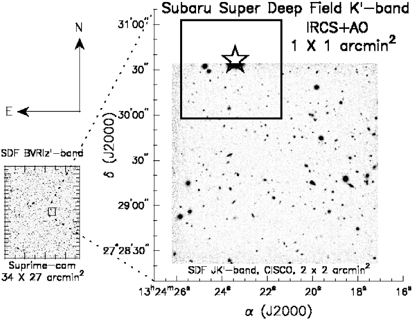
Figure 1.— The location of the Subaru Super Deep Field (SSDF) relative to the Subaru Deep Field (SDF). Intensive observations have been carried out in the SDF using the Subaru Suprime-Cam ($BVRi^{\prime}z^{\prime}$) and the CISCO ($JK^{\prime}$). The stellate symbol in the SSDF shows the location of the AO guide star ($R$ $\sim$ 12).

Our observations were carried out using the Subaru AO system (Takami et al., 2004) and the IRCS (Infra-Red Camera and Spectrograph, Tokunaga et al., 1998; Kobayashi et al., 2000) both mounted on the Cassegrain focus of the Subaru Telescope. The IRCS imager is equipped with a Raytheon Aladdin III 1024$\times$1024 InSb array, offering two pixel scales of 23 and 58 mas for imaging in a wavelength range of 0.9$-$5.5 $\mu$m. We used the pixel scale of 58 mas to cover a wider field of view with the $K^{\prime}$ filter (1.96$-$2.30 $\mu$m, $F_{\lambda}=4.66\times 10^{-10}$ Wm${}^{-2}\mu$m^-1, Tokunaga et al. 2002). The Subaru AO system uses a curvature sensor with 36 control elements, which provides a stellar image of Strehl ratio (the ratio of the observed star peak to the peak value of a perfect telescope diffraction pattern) of $\sim$ 0.28 and full-width at half maximum (FWHM) of $\sim$ 0$\farcs$07 in the $K$ band with an $R\sim 12$ guide star under best observing condition. The improved image quality is expected to increase the detection sensitivity to a point source by $\sim$ 1 mag. However, because AO correction performance degrades with increasing distance from a guide star (see §6.3 for details), the Strehl ratio at the area away from a guide star is lower than the best value. Moreover, since the Strehl ratio should vary with time depending on the observational condition, the resultant Strehl ratio for long exposure time is averaged and lower than the best value. Similarly, the FWHM for long-time exposure image could be broader than the best value at the area away from a guide star. For the present data, the achieved Strehl ratio and the FWHM, which were measured from a point-like source located at 24 arcsec away from the guide star, are 0.1 and 0$\farcs$18 on average, respectively. Because the galaxies in our field of view are distributed within about 40 arcsec away from the guide star, our measured Strehl ratio and FWHM are typical for our observation.

We carried out our observations for a total of nine nights with almost photometric condition. The observing log is given in Table 1. During the observations, we repeated the set of nine-position dithering with a 3$\times$3 grid of 2$\farcs$0 separation. Individual exposure time of 90 or 120 sec was adopted such that the sky background does not saturate the detector well. Since a few bright stars reached saturation even with this short exposure time, residual images following the dithering pattern appeared around the stars due to the memory effect of the InSb array (see grid patterns around bright stars in Figure 3).

Table 1Summary of $K^{\prime}$-band observations.

Date (UT)	Exp. time [sec]	Field
2003/03/17	18630	SSDF
2003/03/18	18000	SSDF
2003/03/19	10800	SSDF
2003/03/20	18480	SSDF
2003/04/22	18630	SSDF
2003/04/23	18630	SSDF
	135	M13 (PSF reference)
2003/04/24	8100	SSDF
	135	M13 (PSF reference)

Throughout each observing night, the variation of the sky background brightness was small except at large airmass. The sky variation corresponds to about $\pm$0.1 mag in the limiting magnitude variation of each frame (Figure 2a), suggesting that the observing condition was almost stable throughout all observing nights. The correction performance of AO changes every moment depending largely on the observational condition. We monitored the variation of spatial resolution by measuring the FWHM of a point-like source which has the sharpest and nearly circular profile in our field of view (marked “S” in Figure 3) except for the saturated bright stars. Since this point-like source “S” is too faint to be detected in each single frame, we combined each set of nine-point dithering to measure the FWHM. The variation of FWHM after AO correction was found to be small for all frames (Figure 2b). Thus, the correction performance of AO was stable and the point spread function (PSF) remained to be constant for each night.

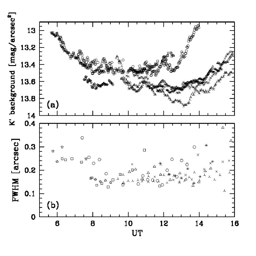
Figure 2.— The variation of the sky background brightness in the $K^{\prime}$ band (a) and the spatial resolution with AO (b) during the observations. Different symbols correspond to different observing nights listed in Table 1. The spatial resolution is represented by the FWHM of the point-like source (“S” in Figure 3).

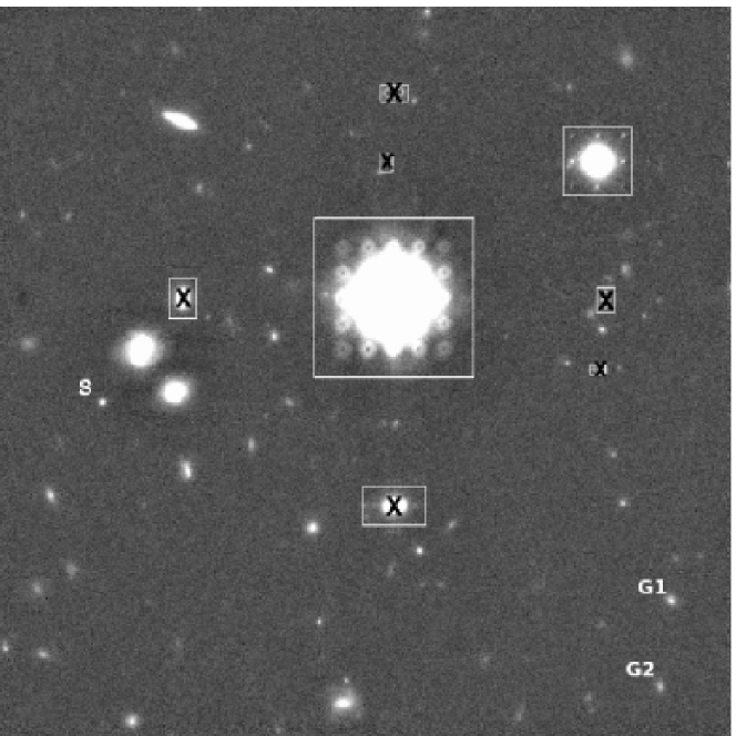
Figure 3.— IRCS+AO $K^{\prime}$-band image of the Subaru Super Deep Field (SSDF) with the total integration time of 26.8 hrs. The field size is 1′ $\times$ 1′ with the pixel scale of 58 mas. The stellar FWHM was measured to be 0$\farcs$18 for the point-like source (indicated by “S” mark). The bright star at the center of the image was used as the AO guide star. Ghosts of bright stars due to the IRCS internal optics (beam splitter and compensator) are indicated by cross marks. The grid patterns around the guide star and other bright objects are the residual image of previous frames due to saturation of the detector. Because of these mock objects, some areas near the bright stars and their ghosts (boxed areas) were excluded from the detection area. G1 is a disk galaxy with an effective radius of 0$\farcs$25, that is the average size of galaxies in the SSDF image (see §6.2). G2 is a galaxy whose radial profile and model fitting are shown in Figure 13.

3. Data reduction

We reduced the data with IRAF software packages. Before the data reduction, we checked all data frames visually and removed some low-signal frames due to cirrus as well as some frames with unusual dark patterns due to unstable detector temperature at the beginning of continuous exposures. We rejected these frames ($\sim$ 15% of all frames) before the data reduction and the resultant total integration time of all used frames is about 26.8 hours. Flat fielding was performed using the median combined sky flat frame. The sky flat frames were created for each night using the dark subtracted raw frames. In generating the sky flat frames, bright and extended objects in each raw frame were masked in order to reduce their contribution to the final flat frame. We made the position map of the bad pixels on the detector from the dark and flat frames, which were used for picking the pixels with extraordinarily high counts and the pixels with extremely low sensitivity, respectively. Bad pixels on our observed frames were removed by interpolation using this position map. The nine frames of each dithering set were median-combined to create the sky frame for each set. Before this process, all of the discernible objects are removed with interpolation by adjacent sky counts to reduce the contribution of the individual objects to the resultant sky level. The sky subtraction was performed for each set of nine-point dithering (every 810 or 1080 seconds) to minimize the effect of time variation of the sky background. Then, we shifted and combined all of the sky subtracted frames with exposure time weighting. The image offsets were determined at a sub-pixel level from the bright objects in each frame. The final $K^{\prime}$ image is shown in Figure 3. The average FWHM of final image was about 0$\farcs$18 for the relatively bright ($K^{\prime}\sim 21.2$) point-like source “S”. Throughout this paper, we used the profile of this point-like source as the PSF of our AO image.

4. Source detection and photometry

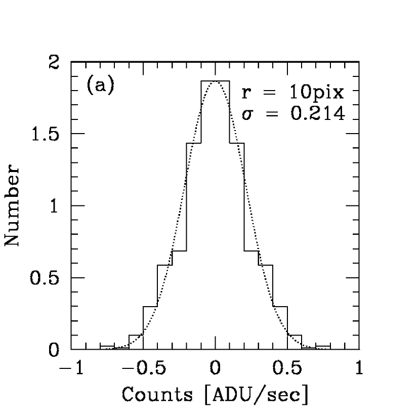
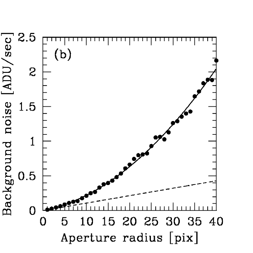
Figure 4.— Measurement of background noise within the aperture. (a) Gaussian function (dotted line) is fitted to the histogram of measured flux in the aperture area $A=\pi r^{2}$ ($r=10$ pixels) which was randomly placed avoiding the object locations. We regarded the width $\sigma$ of gaussian function as the background noise within the aperture. This method allows us to measure the true background noise in which a pixel-to-pixel correlation is taken into account. (b) Relation of aperture radius $r$ versus background noise within the aperture. Filled circles show the measured background noise and the solid line shows the fitted line to the data with a two dimensional function, $ar^{2}+br$, where $a$ and $b$ are the free parameters. The measured background noise with large aperture is significantly larger than that expected from a linear scaling of the pixel-to-pixel noise (dashed line), probably due to the correlated fluctuations of the background on large scale.

Source detection and photometry were performed by the SExtractor (Bertin & Arnouts, 1996). Before the source detection, the final image was smoothed by a gaussian filter ($\sigma$ = 1 pix) to give an optimal source detection capability with less spurious detection. We defined the detection threshold as the 1.5$\sigma$ level of the surface brightness fluctuation of the sky (23.64 mag/arcsec²). If more than 19 contiguous pixels have larger counts than the threshold, we regarded it as a positively detected source. To reduce the risk of spurious detection, some areas near the bright stars and the known ghosts of bright stars are excluded from the detection area (see Figure 3). As a result, the total number of detected sources is 236 within the net detection area of 0.9 arcmin², although some spurious detections due to statistical noise may be included in this number.

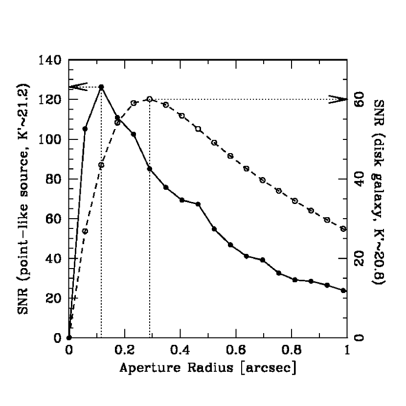
Figure 5.— Signal-to-noise ratio (SNR) of the $K^{\prime}\simeq 21.2$ point-like source “S” (solid line with filled circles, left y-axis) and the $K^{\prime}\ \simeq\ 20.8$ disk galaxy “G1” (dashed line with open circles, right y-axis) as a function of aperture radius. This diagram is used to determine the 5$\sigma$ limiting magnitude. Dotted line shows the maximum SNR and the aperture radius. In case of the point-like source “S”, maximum signal-to-noise ratio of 127 is achieved at aperture radius of 0$\farcs$1, so that the 5$\sigma$ limiting magnitude for point sources is $21.2-2.5\log(5/127)\simeq 24.7$ with an aperture diameter of 0$\farcs$2. Similarly, the 5$\sigma$ limiting magnitude for galaxies was estimated at $K^{\prime}\sim 23.5$ with an aperture diameter of 0$\farcs$6.

We performed photometry of detected sources in terms of aperture magnitude, isophotal magnitude, and total magnitude (see Bertin & Arnouts (1996) for further description of each magnitude). Throughout this paper, we mostly use the total magnitude except for the discussion of size distribution in §7.2, where we use the isophotal magnitude. The photometric calibration was carried out using the infrared faint standard star GSPC P330-E (Persson et al., 1998). We took the image of this standard star at airmass $\simeq$ 1 in a photometric night and used it as the photometric reference for the object frames which were taken in the same night at the same airmass. Then, a bright galaxy ($K^{\prime}\sim 16.9$) in the field was used as the photometric reference for the final image. The resultant zero point in the final combined image is $K^{\prime}\sim 23.645\pm 0.011$ mag/ADU.

Understanding the noise properties is crucial because the limiting magnitude and photometric uncertainty rely on them. The photometric uncertainty in typical near-infrared deep images is well described by the poisson noise of the background signal in each pixel. However, image processing, such as shift and combination, has introduced correlations between neighboring pixels. If the photometric uncertainty was estimated from linear scaling of the pixel-to-pixel variation, we would underestimate it. To estimate the true uncertainty of photometry, we measured the sky fluxes in several tens of circular apertures at random position in the final image and regarded the standard deviation $\sigma$ of the measured fluxes as the photometric uncertainty. We changed the radius of circular apertures ranging from 1 to 40 pixels (0$\farcs$058$-$2$\farcs$3) to cover all the photometric apertures of detected sources (Figure 4). We fitted $\sigma$ with a two-dimensional function of the aperture radius, $\sigma(r)=ar^{2}+br$, where $a$ and $b$ are the fitting parameters. We used this function for calculating the photometric uncertainty of each detected sources with various apertures. The measured uncertainty with this method largely exceeds the uncertainty expected from linear scaling of the pixel-to-pixel noise (dashed line in Figure 4). The large discrepancy at large aperture was also reported in Labbe et al. (2003). This could be caused by correlated fluctuations of the background on large spatial scale.

We estimated the limiting magnitude for point sources using the point-like source “S” in the final image. The limiting magnitude was determined by using a diagram that shows signal-to-noise ratio (SNR) of the point-like-source “S” as a function of an aperture radius (solid line in Figure 5), that was represented as a ratio of flux to photometric uncertainty within an aperture. The achieved 5$\sigma$ limiting magnitude for point sources is $K^{\prime}\sim 24.7$ (5$\sigma$) with an aperture diameter of 0$\farcs$2, where the aperture size was determined to have the maximum SNR. This is the faintest $K$-band limiting magnitude for point sources achieved to date. Because galaxies would have more extended profile than point sources, the limiting magnitude for galaxies should be brighter than that for point sources. Thus, we also estimated a limiting magnitude for galaxies with the similar method as for point sources using a galaxy “G1” (see Figure 3), that is a disk galaxy which has the typical effective radius ($r_{e}=0\farcs 25$) in the SSDF (see §6.2 for details). The achieved 5$\sigma$ limiting magnitude for galaxies is $K^{\prime}\sim 23.5$ (5$\sigma$) for 0$\farcs$6 aperture. The number of detected sources brighter than the limiting magnitude for point sources is 145, while the total number of detected sources is 236 with the faintest magnitude of $K^{\prime}\sim 26.0$.

5. Analysis

5.1. Detection completeness

At the fainter magnitude, the detection completeness decreases because of the statistical noise. We estimated the detection completeness for point sources by conducting the same source detection as described in §4 but with a large number of artificial point sources placed at random positions in the final image. The artificial point sources were created from the point-like source in the final image (source “S” in Figure 3) by applying a flux scaling in the range of $20<K^{\prime}<27$. Thick solid line with filled circles in Figure 6 shows the detection completeness curve for point sources in our final image as a function of $K^{\prime}$ magnitude. We estimated that 50% completeness for point sources is achieved at $K^{\prime}\simeq 25.0$, which means a half of all galaxies can be detected at this magnitude, and it is about 0.6 magnitude deeper than previous deep imaging such as Labbe et al. (2003) and Maihara et al. (2001). Thus, our data should offer the most reliable source detection down to 25 mag. We also estimated the detection completeness for galaxies with artificial galaxies that have the typical size in the SSDF. The artificial galaxies were created to have the same surface brightness profile as the galaxy “G1”, which was used in the limiting magnitude estimation in §4. We placed them at random positions with varied flux in the range of $20<K^{\prime}<27$. Figure 7 shows the estimated detection completeness curve for galaxies. The completeness curve for galaxies in our final image are shown as thick solid line with filled circles. For a comparison, the completeness curve for extended source in the previous deep imaging by Maihara et al. (2001) is also shown as thin dashed line with stellate symbols in the same diagram. We estimated that 50% completeness for extended source is achieved at $K^{\prime}\simeq 24.1$, that is about 0.6 mag fainter than that of Maihara et al. (2001). This magnitude gain is same as for the gain for point source, suggesting that the AO system improves the efficiency of detecting high-redshift galaxies as well as that of point sources. In this paper, the detection completeness for point source is used to correct the number counts. Therefore, the detection completeness here should be considered upper limits and then the corrected counts should be considered lower limits.

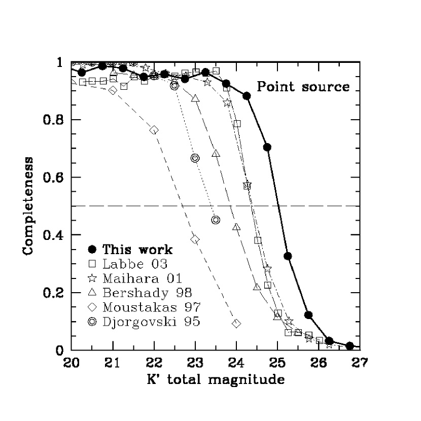
Figure 6.— Detection completeness curves derived from the simulations using the artificial point sources. Thick solid line with filled circles shows the detection completeness for point source of our $K^{\prime}$ survey in the SSDF, while thin lines with other symbols show that of deep $K$ or $K^{\prime}$ imaging surveys from the literature (Labbe et al., 2003; Maihara et al., 2001; Bershady et al., 1998; Moustakas et al., 1997; Djorgovski et al., 1995). Horizontal dashed line indicate the level of 50% completeness.

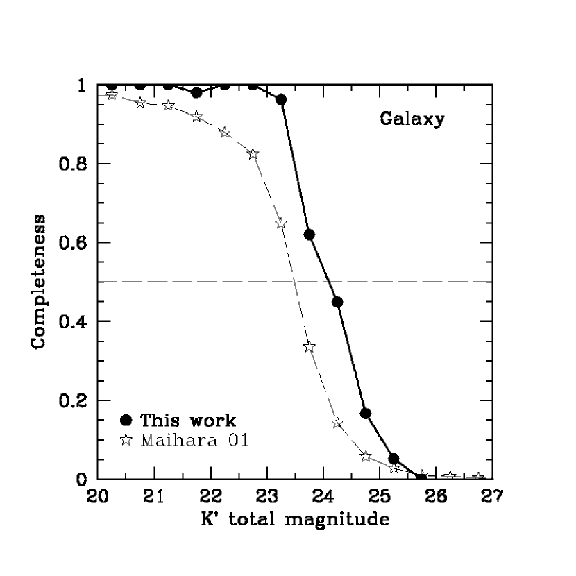
Figure 7.— Detection completeness curves derived from the simulations using the artificial galaxies that have the typical size in the SSDF. Thick solid line with filled circles shows the detection completeness for galaxies of our $K^{\prime}$ survey in the SSDF, while thin dashed line with stellate symbols show that of Maihara et al. (2001) for a comparison. Horizontal dashed line indicate the level of 50% completeness.

5.2. Noise contamination to number counts

We detected the objects down to $K^{\prime}<26$ in our final image. Based on the photometric measurements of these objects, we derived the number counts in the 0.5 magnitude bin (Table 2). The number counts, in principle, contain not only the counts from galaxies, but also the counts from the Galactic stars and spurious detections due to the effect of statistical noise. The contribution of the Galactic stars to our number counts should be negligible, because the expected star counts toward the Galactic pole are less than 0.2 mag^-1acrmin^-2 in all magnitude range (Minezaki et al., 1998b; Fugal & Moody, 2003). On the other hand, the contribution of spurious detection is significant in the faint end, where the signal-to-noise ratio for the detection becomes lower. We estimated the number of spurious detections from an artificial noise frame which was created by combining the sky subtracted frames without adjusting the dithering offset. The combination was conducted with the options of exposure time weighting, which is similar to the combination of the final image. Before the combination, all discernible objects in each image were removed by interpolation and the estimated noise from the adjacent pixels was added on the interpolated pixels. Even after removing the discernible objects, even fainter objects could be remained in the noise in each single frame. In order to minimize the contribution of the light from such faint objects, the sign of each image was reversed before the combination. We applied the same detection procedure to the artificial noise image as used for the source detection. The resultant number of spurious detections in each 0.5 magnitude bin is given in Table 2. We derived the galaxy number count in each magnitude bin by subtracting the number of spurious detection from the raw count. The estimated galaxy counts are listed in Table 2 and shown in Figure 8.

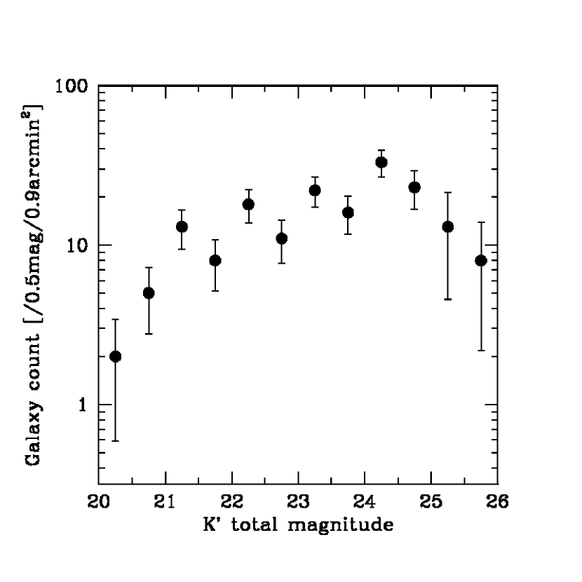
Figure 8.— Galaxy counts in the SSDF in the 0.5 magnitude bin without any correction except for subtraction of the noise contamination. Error bars show the uncertainties due to the poisson statistics.

Table 2The corrected $K^{\prime}$-band galaxy number counts.

$K^{\prime}$	$n_{raw}$	$n_{noise}$	$n_{gal}$	$\Delta n_{gal}^{p}$	$\Delta n_{gal}^{p+c}$	Completeness	$N_{cor}$	$\Delta N_{cor}$
(1)	(2)	(3)	(4)	(5)	(6)	(7)	(8)	(9)
20.25	2	0	2	1.41	1.51	0.96	1.959E4	1.287E4
20.75	5	0	5	2.24	2.59	0.99	4.837E4	2.157E4
21.25	13	0	13	3.61	4.97	0.98	9.735E4	4.168E4
21.75	8	0	8	2.83	3.54	0.95	9.112E4	3.067E4
22.25	18	0	18	4.24	6.39	0.96	1.360E5	5.479E4
22.75	11	0	11	3.32	4.44	0.94	1.253E5	3.871E4
23.25	22	0	22	4.69	7.47	0.96	1.598E5	6.367E4
23.75	17	1	16	4.24	6.06	0.92	2.100E5	5.377E4
24.25	37	4	33	6.40	11.15	0.88	2.497E5	1.038E5
24.75	31	8	23	6.24	9.47	0.70	2.577E5	1.104E5
25.25	42	29	13	8.43	10.30	0.33	3.038E5	2.587E5
25.75	21	13	8	5.83	8.32	0.12	4.746E5	5.575E5

Note. — (1) $K^{\prime}$-band total magnitude. (2) Raw counts of detected objects in the 0.5 magnitude bin. (3) Noise counts in the 0.5 magnitude bin. (4) Galaxy counts in the 0.5 magnitude bin ($n_{gal}=n_{raw}-n_{noise}$). (5) Uncertainties in the galaxy counts coming from poisson statistics. (6) Uncertainties in the galaxy counts coming from poisson statistics and clustering of galaxies. (7) Detection completeness for point source. (8) Differential galaxy number counts in mag^-1deg^-2 corrected for the incompleteness and the scatter due to the photometric uncertainties. (9) Uncertainty in the corrected differential number counts coming from the poisson statistics and the clustering of galaxies.

5.3. The scatter of number counts due to photometric uncertainty

Even if the noise counts are removed, the scatter of galaxy number counts among magnitude bins still remains due to photometric uncertainty. In order to evaluate the effect of this scatter, we performed a simulation by adding artificial objects to the final image and applying the same detection procedure as described in §4. In this simulation, about 10 artificial objects were added 450 times (total of about 4,500 objects) in order not to largely change the number density of the objects in the final image and the detection procedure was performed each time. The artificial objects of various magnitudes were created from the point source in the final image by scaling its flux. The magnitudes of the artificial objects were assumed to distribute with power-law, $N(m)\propto 10^{\alpha m}$, where $N$ is the number of the artificial objects in each 0.5 magnitude bin, $m$ is the central magnitude of each magnitude bin, and $\alpha$ is the power-law index. We performed the simulation only with point sources because previous analyses related to the number counts are based on point sources to give the lower limit of the counts. An initial power-law index of ${\alpha}_{0}=d\log N/dm$ was assumed to be the slope of raw galaxy counts over a reliable magnitude range, $22<K^{\prime}<24$, where the signal-to-noise ratio is greater than 3 (i.e. more than 10 raw counts) and the detection completeness for point sources is higher than 90%.

Based on the simulation, we first generated the transfer matrix $T_{ij}$, each element of which gives the fraction of galaxies with magnitude $m_{j}$ but detected with $m_{i}$. Then, we generated the probability matrix $P_{ji}$, each element of which gives the probability that an artificial object detected with $m_{i}$ actually has a magnitude of $m_{j}$. These elements are described as

$$P_{ji}=T_{ij}n_{j}/\sum_{k}T_{ik}n_{k}\ ,$$ (1)

where $n_{j}$ is the number of the artificial objects with magnitude $m_{j}$. The probability matrix is shown in Figure 9. With this probability matrix, we corrected the galaxy number counts as

$$n^{cor}_{j}=\sum_{i}P_{ji}n^{gal}_{i}\ ,$$ (2)

where $n^{cor}_{j}$ is the corrected galaxy number count at magnitude $m_{j}$, and $n^{gal}_{i}$ is the raw galaxy count with detected magnitude $m_{i}$ (Table 2). If the slope of corrected galaxy counts was different from the initial slope ${\alpha}_{0}$ used in the simulation, the correction procedure described above was repeated with different initial slope until the corrected slope coincides with the initial slope. This method has been employed in some studies of galaxy number counts (Smail et al., 1995; Minezaki et al., 1998a; Maihara et al., 2001).

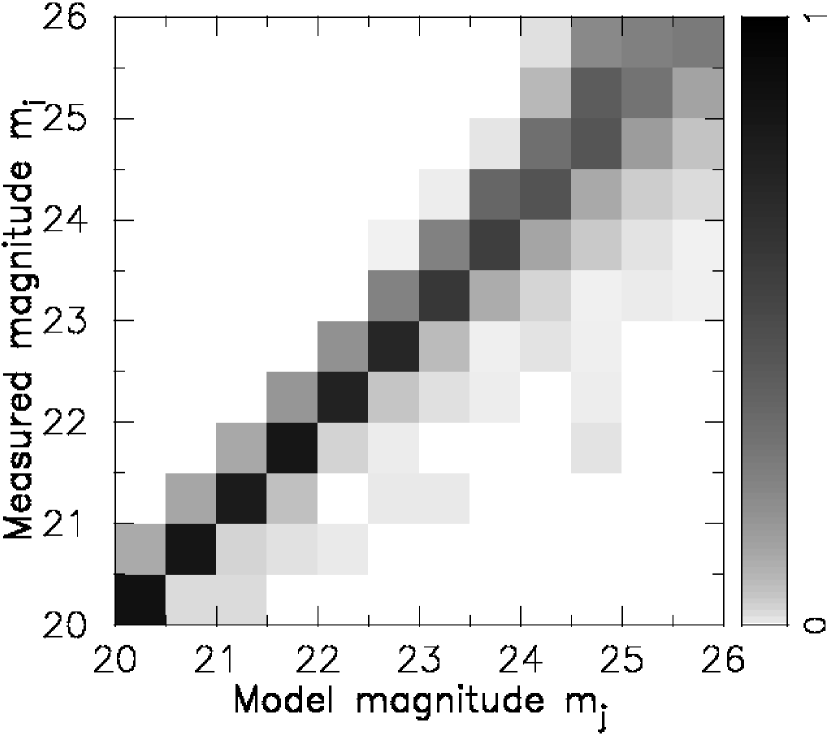
Figure 9.— The probability matrix for detected galaxies in the SSDF based on the simulation using the artificial point sources. Each element of the matrix gives the probability that a galaxy detected with $m_{i}$ actually has a model magnitude of $m_{j}$. The probability is color-coded according to the scale bar on the right of this figure.

We derived the differential galaxy number counts ($N^{cor}_{i}$) in the unit of number mag^-1 deg^-2 from the counts $n^{cor}$ after correcting for the detection completeness estimated for point source in §5.1 (Table 2). Figure 10 shows the plot of galaxy number counts with and without the completeness correction. At brighter magnitude ($K^{\prime}<22.0$), our differential number counts are not complete with less than 3$\sigma$ measurements (i.e. less than 9 raw counts) because of a small field of view (1′$\times$ 1′). At fainter magnitude, the detection completeness for point source becomes lower than 50% at $K^{\prime}>25$. Thus, the reliable magnitude range of our differential number counts is $22<K^{\prime}<25$.

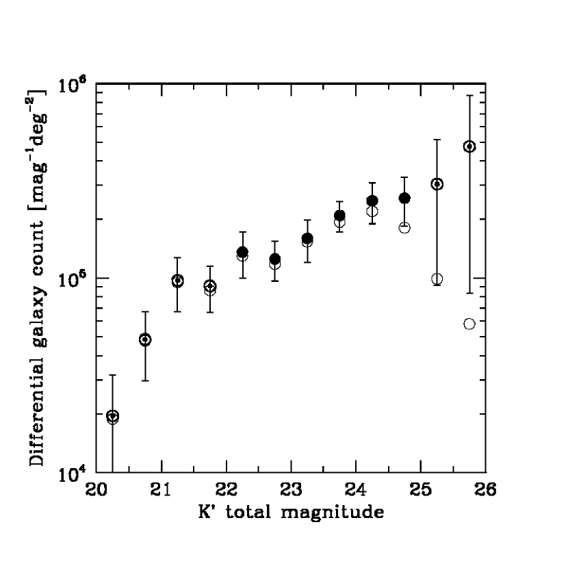
Figure 10.— Differential $K^{\prime}$-band number counts of galaxies estimated from the galaxy counts in the SSDF. Filled circles show the galaxy counts in a reliable magnitude range of $22<K^{\prime}<25$, where the signal-to-noise ratio for raw counts is greater than 3 and the detection completeness for point source is higher than 50%. Circled dots show the less reliable galaxy counts. These galaxy counts are corrected for the detection completeness and the scatter due to the photometric uncertainty. Open circles show the galaxy counts without completeness correction. The completeness correction becomes significant at $K^{\prime}>25$. Error bars show the uncertainties due to the poisson statistics.

5.4. Field-to-field variations of galaxy number counts

Clustering of galaxies could lead to the systematic uncertainties in the number counts. We estimated the field-to-field variations of the counts due to the clustering from an angular correlation function. Considering an angular area of $\Omega$, with a mean count of $\langle N\rangle$ galaxies, the variance in the number of detected galaxies is

$$\mu_{2}=\langle N\rangle+\frac{\langle N\rangle^{2}}{\Omega^{2}}\int\int\omega(\theta_{12})\,d\Omega_{1}d\Omega_{2}\ ,$$ (3)

where $\omega(\theta)$ is the angular correlation function of galaxies and $\theta_{12}$ is the angle between the solid-angle elements $d\Omega_{1}$ and $d\Omega_{2}$ (Groth & Peebles, 1977). In this formula, first term comes from poisson statistics and second term comes from the clustering. The angular correlation function for faint galaxies has been measured in the $K$ band in a number of literatures (e.g., Baugh et al. 1996; Carlberg et al. 1997; Roche et al. 1999), and it is described in a form of $\omega(\theta)=A\theta^{-0.8}$. The amplitude $A$ at fixed $\theta$ is a decreasing function of $K$ magnitude, while there is an evidence that the amplitude becomes relatively flat at $K>20$ with a value of $A\sim 1.1\times 10^{-3}$ when $\theta$ is measured in degree (Roche et al., 1999). In this paper, we assume the amplitude-magnitude relation does not turn over at $K>20$, which is theoretically reasonable (e.g., Roche & Eales 1999), to set the upper limit on the uncertainty of the counts coming from the clustering of galaxies. For the 0.9 arcmin² area of the SSDF, the variance becomes $\langle N\rangle+61.3A\langle N\rangle^{2}$. The estimated uncertainties of the galaxy counts coming from poisson statistics and clustering at each magnitude bin are summarized in Table 2. The uncertainties due to poisson statistics and clustering are not much larger than that only due to poisson statistics.

In order to check the validity of the variation estimated from the angular correlation function, we also estimated the field-to-field variations of the counts using the SDF data (Maihara et al., 2001), which has almost four times larger area (1$\farcm$97 $\times$ 1$\farcm$9) than that of the SSDF. We derived the counts from four discrete 0.9 arcmin² areas in the SDF at $20<K^{\prime}<23$ where the detection completeness is higher than 90% for both of the SDF and the SSDF. The galaxy counts of the SSDF are plotted in Figure 11 with the uncertainties estimated from equation (3). The galaxy counts for four discrete areas in the SDF are also plotted. It is found that the uncertainties due to the poisson statistics and the clustering of galaxies are almost consistent with the variations of the galaxy counts from four areas in the SDF.

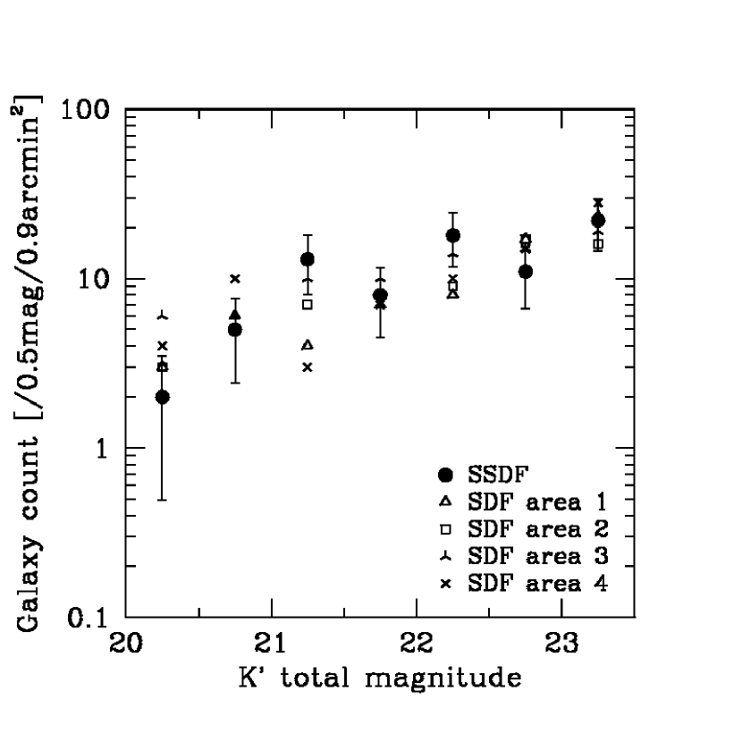
Figure 11.— The galaxy counts in the SSDF with the uncertainties due to the poisson statistics and the clustering of galaxies estimated from the angular correlation function for the 0.9 arcmin² area of the SSDF (filled circles). The galaxy counts for four discrete 0.9 arcmin² areas in the SDF are also plotted (open circles). The estimated uncertainties of the SSDF due to a poisson statistics and a clustering are almost consistent with the variance of the galaxy counts for four areas in the SDF.

6. Performance of AO deep imaging

6.1. Comparison with seeing-limited observation

To estimate the performance of our AO deep imaging, we compared the quality of our AO image of the SSDF to that of the seeing-limited image of the SDF (Maihara et al., 2001). The SDF data were obtained by the Subaru/CISCO under the FWHM$\sim$0$\farcs$45 seeing condition with the total integration time of 9.7 hours. Because a part of the SDF field of view is included in the SSDF (see Figure 1), we can make a direct comparison between AO and seeing-limited data.

Figure 12 shows the encircled flux plot of the point sources detected in the SSDF and the SDF. The 50% of the total flux is contained within a radius of 0$\farcs$18 for the SSDF, while 0$\farcs$27 for the SDF. The higher flux concentration due to the AO correction resulted in much higher sensitivity. To estimate the sensitivity gain for our AO observation against seeing-limited observation, we derived the 5$\sigma$ limiting magnitude for point sources in the SSDF and in the SDF with the same method as described in §4. The 5$\sigma$ limiting magnitude is about 22.9 (0$\farcs$2 aperture) for the SSDF and 22.4 (0$\farcs$4 aperture) for the SDF with an hour integration time. Thus, the sensitivity gain due to AO correction is about 0.5 mag in the $K^{\prime}$ band.

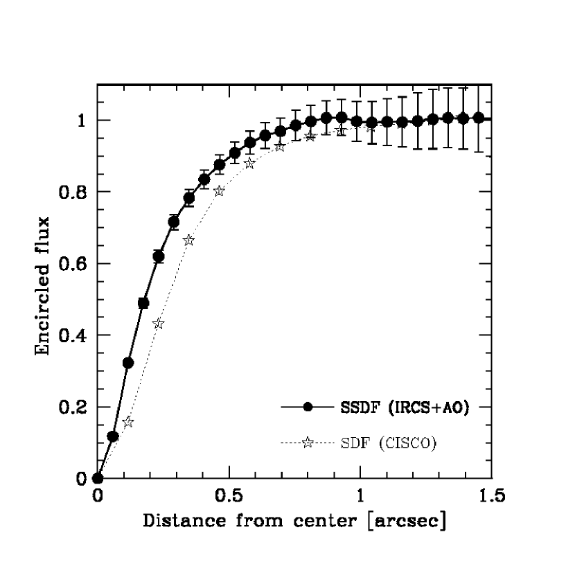
Figure 12.— Encircled flux of the point-like source “S” in the SSDF (filled circles) as a function of distance from the center of the stellar image. For a comparison, encircled flux of a point source in the SDF (stars, Maihara et al., 2001) is also shown. Since there is no point source in the overlapped region between the SSDF and the SDF, a different point source is used for the SDF. Total flux was normalized to unity for both point sources. Vertical error bars show the photometric uncertainties in each aperture. Because the point-like source “S” in the SSDF is much fainter than the point source used for the SDF, the photometric uncertainties for the SSDF data are much larger than that for the SDF data. Much higher concentration of flux was attained in the SSDF compared to the SDF.

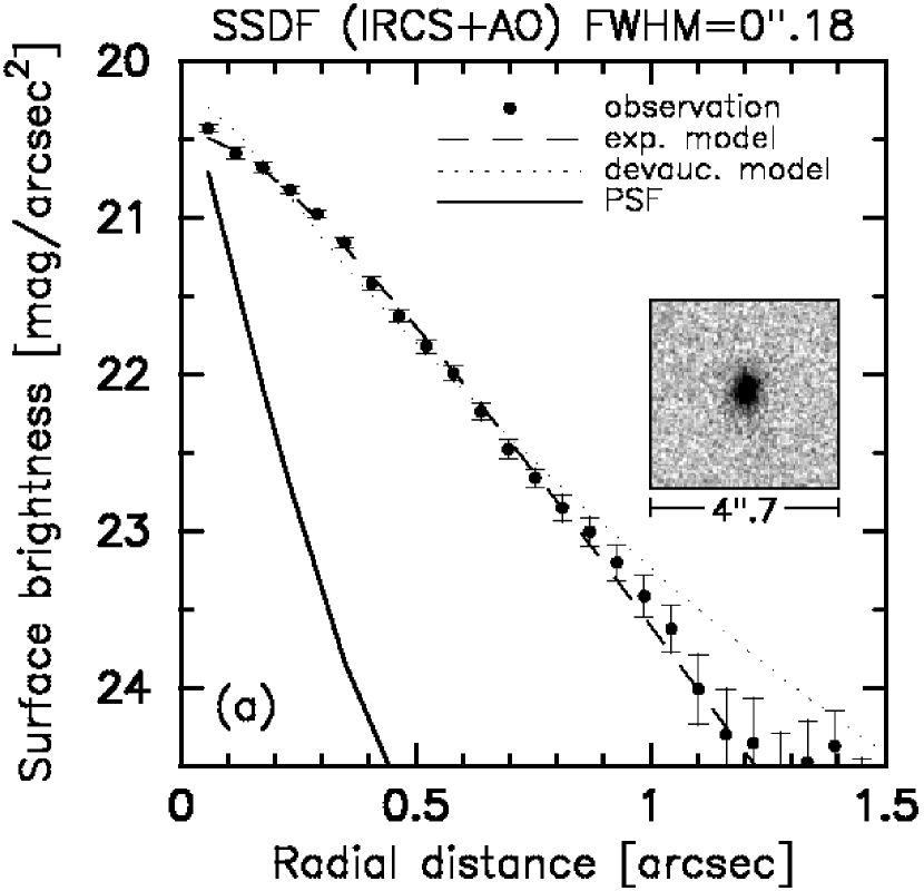
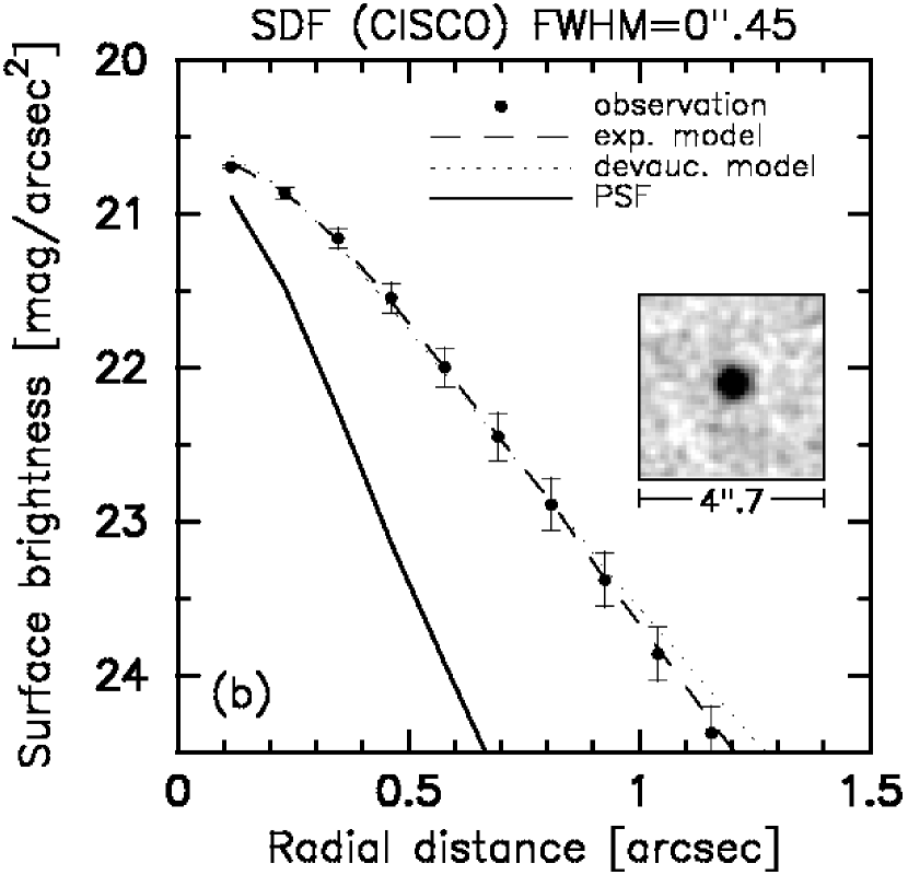
Figure 13.— Radial profile fitting to a $K^{\prime}\sim 21.3$ galaxy at $z\sim 1.46$ (“G2” in Figure 3) in (a) the SSDF with IRCS+AO and (b) the SDF with CISCO (Maihara et al., 2001). Filled circles show the observed data in both figures. The PSF-convolved de Vaucouleurs (dotted line) and exponential (dashed line) profiles were used to model a galaxy dominated by bulge and disk, respectively. Solid lines show the PSF profile in both figures. The high-resolution (FWHM = 0$\farcs$18) image of the SSDF clearly shows that the best fitted model is the exponential (disk dominated) profile, while it is difficult to distinguish the two models with the seeing-limited image of the SDF because of the large FWHM (= 0$\farcs$45).

The improvement of spatial resolution with AO is also significant. Figure 13 shows a model fit to the surface brightness profile of a $K^{\prime}\sim 21.3$ galaxy at $z\sim 1.46$ (“G2” in Figure 3), using a PSF-convolved de Vaucouleurs profile (de Vaucouleurs, 1948) for a bulge-dominated galaxy and an exponential profile (Freeman, 1970) for a disk-dominated galaxy. While it was difficult to distinguish these model profiles for the seeing-limited SDF data, this galaxy is evidently a disk dominated galaxy for our SSDF data. Effective radii of local galaxies, except for compact dwarf galaxies, range from $\sim$1.0 kpc to $\sim$ 10 kpc depending on their luminosity (Bender et al., 1992; Impey et al., 1996). Since our spatial resolution of 0$\farcs$18 corresponds to about 1.4 kpc at $z\sim 1$, we can determine the size as well as the morphological type even at $z>1$. Thus, our AO morphology data should enable systematic and quantitative study of rest-frame optical morphology of galaxies at $z>1$ (Minowa et al. 2005, in preparation).

6.2. Effect of partially corrected PSF

Typical AO system operated with a guide star of moderate brightness can only partially correct for turbulence-induced distortions. The partially corrected PSF consists of two components: a diffraction-limited core superimposed on a seeing halo. As the Strehl ratio becomes lower, which means a decrease of the degree of correction, a greater proportion of energy in the diffraction-limited core is scattered into the surrounding halo and the peak of the diffraction-limited core becomes lower. As a result, the seeing halo becomes the dominant component in the PSF. For the present SSDF data with the Strehl ratio of about 0.1, since about 90% of the energy is scattered into the surrounding halo, the FWHM of the observed PSF ($\sim 0\farcs 18$) is broader than the diffraction-limited core ($\sim 0\farcs 057$ in the $K$-band) and the wings extended out to the seeing size are seen around the edge of the PSF (see Figure 14).

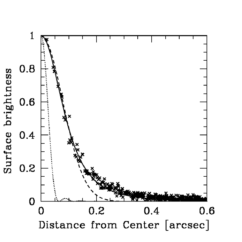
Figure 14.— Radial profile of the observed PSF in the SSDF. The peak surface brightness of the PSF is normalized to unity. The moffat profile (solid line) and the gaussian profile (dashed line) are fitted to the observed PSF. The moffat profile represents well the observed PSF, while the gaussian profile only represents the central part of the observed PSF and failed to represents the extended wings. The observed PSF has a broader FWHM than the Subaru diffraction-limited PSF (dotted line) because of the low Strehl ratio ($\sim$ 0.1).

The surface brightness profile of galaxies detected in the SSDF may be distorted by the extended wings of the observed PSF. To estimate the effect of the extended wings of the observed PSF on the flux and size measurement of the galaxies in the SSDF image, we conducted a simulation using artificial galaxies that were convolved with a model PSF profile. Figure 14 shows the radial profile of the observed PSF and the fitted lines with a moffat profile and a gaussian profile. These profiles are described as

$$I(r) = \left[1+(2^{1/\beta}-1)\left(2r/FWHM\right)^{2}\right]^{-\beta}\ \ (moffat),$$ (4a)

$$I(r) = \exp\left[-\ln(2)\left(2r/FWHM\right)^{2}\right]\ \ (gaussian),$$ (4b)

where $r$ is the distance from the center of the PSF, $FWHM$ is the full width at half maximum of the PSF and $\beta$ is the constant related to the shape of the profile. As $\beta$ decreases, the moffat profile deviates from the gaussian profile and comes to show more extended wings. For the observed PSF in the SSDF, best fit parameters of $FWHM$ and $\beta$ are 0$\farcs$18 and 1.73, respectively. We found that the moffat profile represents well the observed PSF, while the gaussian profile fails to represents the extended wings of the observed PSF (see Figure 14). Thus, we used the fitted moffat profile to convolve the artificial galaxies in the simulation. The artificial galaxies are created to have the typical size in the SSDF image. Figure 15 shows an isophotal area of the observed galaxies, that means the area where the surface brightness of the galaxies is brighter than the detection threshold of 23.64 mag/arcsec², as a function of the isophotal magnitude. We also plotted the isophotal areas of the simulated disk galaxies with $r_{e}=$ 0$\farcs$1, 0$\farcs$25, and 0$\farcs$5. Because the sizes of the observed galaxies are roughly distributed between the size distribution of the simulated disk galaxies with 0$\farcs$1 and 0$\farcs$5, we used the disk galaxy with the intermediate size of $r_{e}=0\farcs 25$ as the artificial galaxy that models the typical galaxies in the SSDF image. The size and morphological type of the artificial galaxies are same as the galaxy “G1”, which was used to estimate the limiting magnitude and the detection completeness for galaxies (see §4 and §5.1). After we placed the artificial galaxies at random positions in the SSDF image with varying their fluxes, we measured their magnitude and isophotal area with the same technique as used for the observed galaxies.

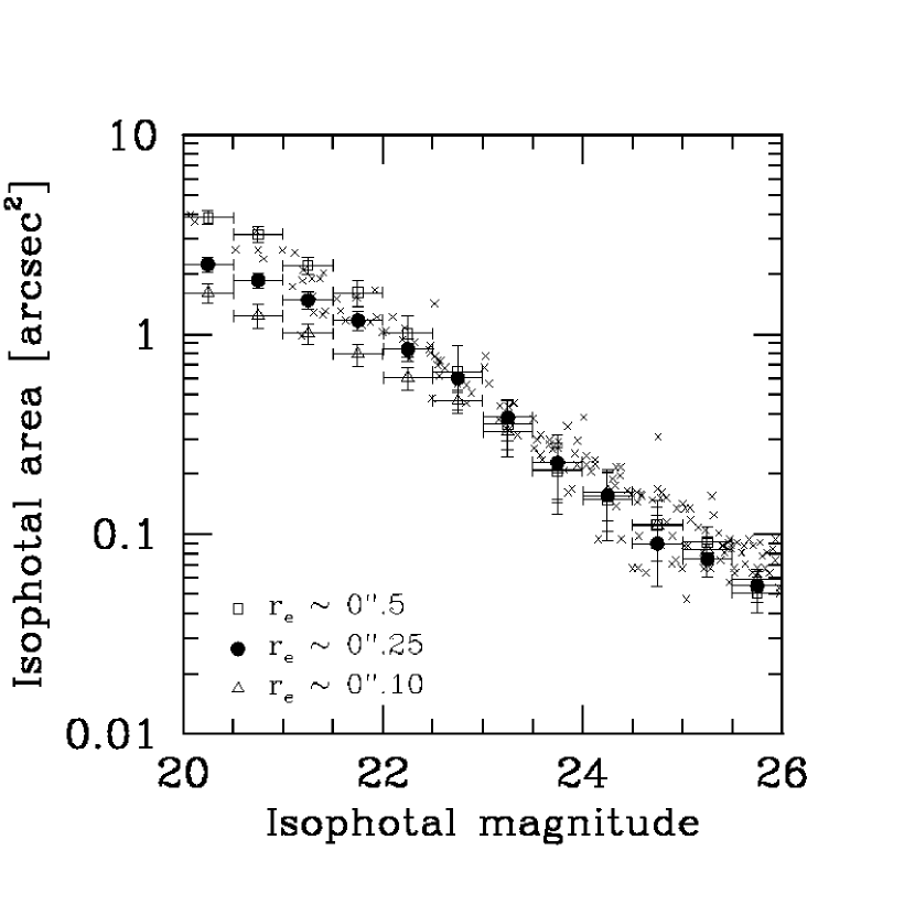
Figure 15.— The isophotal area versus isophotal magnitude diagram for the observed galaxies (crosses). We also plotted the mean isophotal area for the simulated disk galaxies with effective radius ($r_{e}$) of 0$\farcs$.1 (open triangles), 0$\farcs$25 (filled circles), and 0$\farcs$5 (open squares). The horizontal error bars show the bin size around the mean and the vertical error bars show the $1\sigma$ dispersion of the isophotal area of the simulated galaxies. The simulated disk galaxies are convolved with the observed PSF modeled by the moffat profile. The isophotal areas of the observed galaxies are roughly distributed between that of the simulated disk galaxies with $r_{e}=0\farcs 1$ and $0\farcs 5$. Thus, we used the disk galaxy with the intermediate size of $r_{e}=0\farcs 25$ as the artificial galaxy that models the typical galaxies in the SSDF image.

Figure 16 shows a comparison between the model magnitude and the measured magnitude (total and isophotal) of the artificial galaxies. The measured total and isophotal magnitudes are almost consistent with the model magnitude within the uncertainties, although the measured magnitude of the artificial galaxies at the faint end tend to be slightly fainter than the model magnitude. Thus, the extended wings of the observed PSF should not affect the measurement of the magnitude of the typical galaxies in the SSDF image.

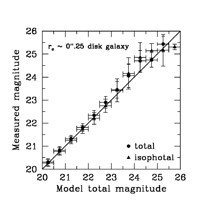
Figure 16.— Comparison between the model magnitude and the measured magnitude of the artificial galaxies that have the typical size in the SSDF image (see Figure 15). Filled circles show the total magnitude and filled triangles show the isophotal magnitude. Solid line shows where the model magnitude is equal to the measured magnitude. The measured total and isophotal magnitudes are almost equal to the model magnitude.

Figure 17(a) shows the isophotal area of the artificial galaxies with $r_{e}=0\farcs 25$ as a function of the isophotal magnitude. We also show the isophotal area versus isophotal magnitude diagram for small galaxies with $r_{e}=0\farcs 1$ in Figure 17(b) for a comparison. To estimate the effect of the extended wings of the observed PSF on the galaxy size measurement, we compared the isophotal area of the artificial galaxies convolved with the moffat profile and that convolved with the gaussian profile. Both of the profiles were fitted to the observed PSF. The moffat profile represents well the observed PSF that have extended wings, while the gaussian profile only represents the central part of the observed PSF (see Figure 14). The isophotal areas of the $r_{e}=0\farcs 25$ galaxies convolved with the moffat profile are almost consistent with those convolved with the gaussian profile at all magnitude range. On the other hand, the isophotal areas of the $r_{e}=0\farcs 1$ galaxies convolved with the moffat profile are larger than that convolved with the gaussian profile. These implies that the extended wings of the observed PSF should not affect the isophotal area of the typical galaxies in the SSDF image, while it may affect the isophotal area of small galaxies at the bright magnitude range.

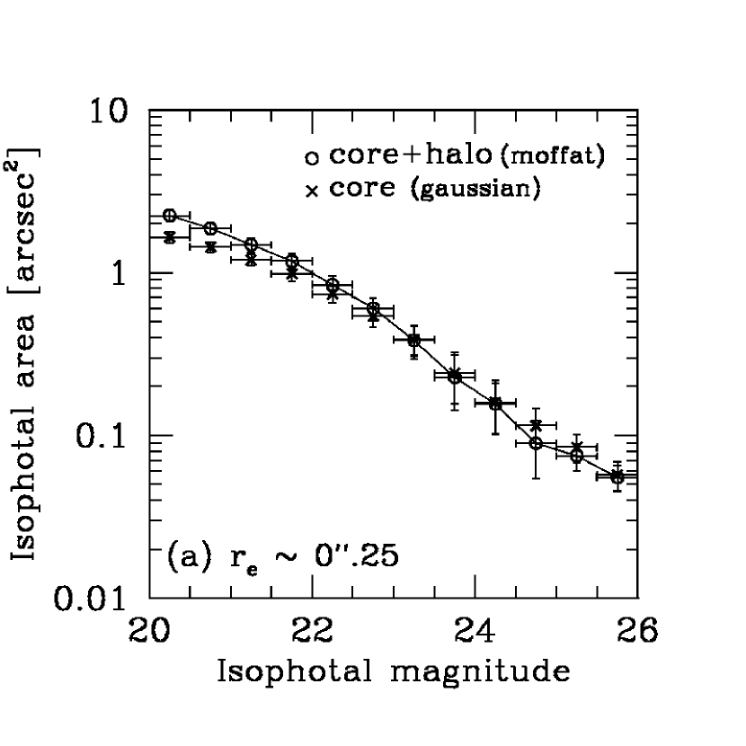
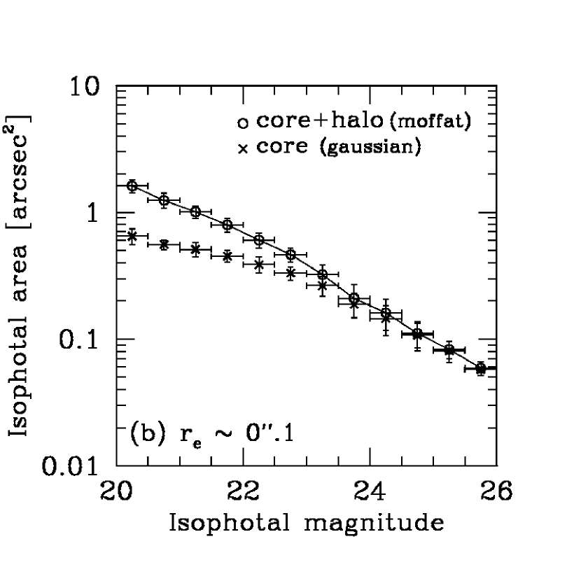
Figure 17.— The isophotal area of the artificial galaxies are shown as a function of their isophotal magnitude ($m_{iso}$). Left panel (a) shows the case for disk galaxies with effective radius ($r_{e}$) of 0$\farcs$25, which is the typical size in the SSDF. We also show the same diagram for smaller disk galaxies with $r_{e}=0\farcs 1$ in right panel (b) for a comparison. The artificial galaxies are convolved with a moffat profile (open circles) and a gaussian profile (crosses). The moffat profile represents well the observed PSF that have extended wings, while the gaussian profile only represents the central part of the observed PSF. The isophotal area of the $r_{e}=0\farcs 25$ galaxies convolved with the moffat profile is not much different from that convolved with the gaussian profile. On the other hand, the isophotal area of the $r_{e}=0\farcs 1$ galaxies convolved with moffat profile is larger than that convolved with the gaussian profile at $m_{iso}\leq 23$.

6.3. Effect of angular anisoplanatism

The performance of AO correction degrades gradually with increasing distance from a guide star. This is due to increased decorrelation of the turbulence-induced aberration away from the location of the guide star (angular anisoplanatism, e.g. Hardy 1998). Therefore, spatial resolution (thus sensitivity) is usually highest in the region close to the guide star and decreases gradually as we go farther away from it.

The angular anisoplanatism in our imaging data was evaluated from some snapshots of globular cluster M13 using AO, in which a number of stars are distributed uniformly in our 1′ $\times$ 1′ field of view. The snapshots were taken just after the deep imaging so that the observational condition does not change significantly (Table 1). The AO guide star for the snapshots was selected to have the same brightness as that of the deep imaging. Figure 18a shows the variation of the stellar FWHM (spatial resolution) with respect to the distance from the guide star. Similarly, Figure 18b shows the variation of the 5$\sigma$ limiting magnitude with an hour integration (sensitivity) in the field. The stellar FWHM and the limiting magnitude deteriorate with increasing distance from the guide star.

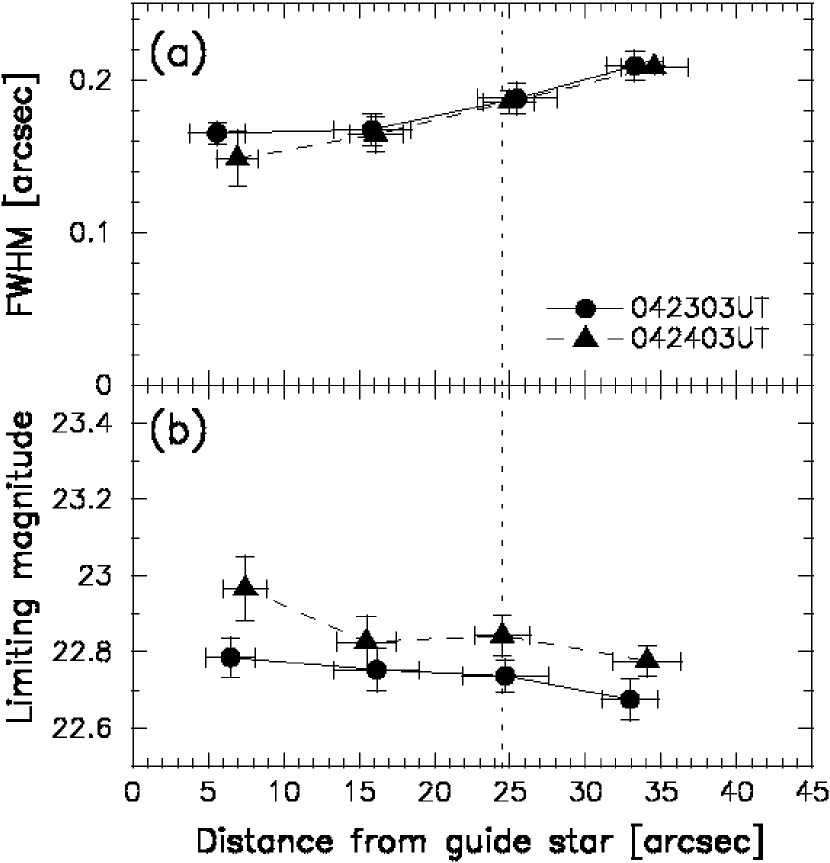
Figure 18.— Variation of (a) the FWHM of point sources (spatial resolution) and (b) the $5\sigma$ limiting magnitude with an hour integration. The results as a function of distance from a guide star were based on the snapshots of a globular cluster M13 which were taken just after the deep imaging on 2003 April 23 (filled circles) and 24 (filled triangles) in Universal Time. Vertical dotted line shows the location of the reference point-like source (“S” in Figure 3), from which the FWHM and $5\sigma$ limiting magnitude of the SSDF were derived (see §3). Most of detected galaxies in the SSDF are distributed in a range of distance from 10″ to 35″, and the effect of anisoplanatism should be negligible in this range.

The stellar FWHM and the 5$\sigma$ limiting magnitude in the SSDF are 0$\farcs$18 and $K^{\prime}\sim 22.9$ with an hour integration, respectively, for the point-like source located at the distance of 24″ from the guide star (dotted line in Figure 18). Since more than 90% of the detected galaxies in the SSDF are distributed in a range of distance from 10″ to 35″, the uncertainties in measurements of the stellar FWHM and the 5$\sigma$ limiting magnitude due to anisoplanatism are about $\pm$0$\farcs$03 and $\pm$0.1 mag, respectively, which should be negligible for the following discussions.

7. Discussion

7.1. Galaxy number counts

Figure 19 shows our differential number counts of galaxies in the reliable magnitude range of $22<K^{\prime}<25$, where the signal-to-noise ratio for raw counts is greater than 3 and the detection completeness for point source is more than 50%. The count slope $\alpha\equiv d\log N/dm$ is about 0.15 $\pm$ 0.08, where the uncertainty was defined as the uncertainty in the least-square fitting to the data. For a comparison, other $K$ and $K^{\prime}$ band number counts in the literatures are also shown in Figure 19 and summarized in Table 3. In this paper, we made no distinction between $K$ and $K^{\prime}$  because the magnitude difference is expected to be $\langle K^{\prime}-K\rangle\lesssim 0.03$ (Minezaki et al., 1998a), which is negligible.

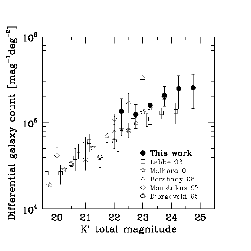
Figure 19.— Differential $K^{\prime}$-band number counts of galaxies estimated from the SSDF galaxy counts in the reliable magnitude range (filled circles) where the signal-to-noise ratio for raw counts is more than 3 and the detection completeness for point source is more than 50%. Error bars for this work show the uncertainties due to a poisson statistics and a clustering of galaxies estimated from an angular correlation function. For a purpose of comparison, the counts in the literatures are also plotted. Their magnitude ranges are limited by the same reliability criteria as ours.

Table 3The comparison of the SSDF with other deep surveys in the $K$ band.

Survey	Instrument	Integration time	Area	$m_{50}$	$\alpha$	mag range
		[hours]	[arcmin2]
This work (SSDF)	Subaru/IRCS+AO	26.8	1.00	25.0	0.15	22$-$25
Labbe et al. 2003 (FIRES)	VLT/ISAAC	35.6	6.25	24.4	0.15	22$-$24
Maihara et al. 2001 (SDF)	Subaru/CISCO	9.7	4.00	24.4	0.23	20$-$24
Bershady et al. 1998	Keck/NIRC	4.9	1.50	24.0	0.36	19.5$-$22.5
Moustakas et al. 1997	Keck/NIRC	1.7	2.41	22.7	0.23	18$-$23
Djorgovski et al. 1995	Keck/NIRC	5.6	0.44	23.5	0.32	20$-$24

Our counts at $23<K^{\prime}<24.5$ are in good agreement with those of the SDF (Maihara et al., 2001), although these counts at $22<K^{\prime}<23$ differ by a factor of 1.2$-$1.6. Earlier results of the $K$-band deep imaging by the Keck telescope reported the slope of 0.23 (Moustakas et al., 1997), 0.32 (Djorgovski et al., 1995), and 0.36 (Bershady et al., 1998) at $20<K^{\prime}<23$, respectively. The discrepancy of the faint-end slopes could be originated from the difference in the adopted technique of incompleteness correction. The HDF-S deep imaging (FIRES, Labbe et al., 2003) shows that the count slope changes from $\alpha\,\simeq\,0.25$ at $20<K^{\prime}<22$ to $\alpha\,\simeq\,0.15$ at $22<K^{\prime}<24$. The break of the count slope at the faint end had not been seen in other deep $K$-band imaging surveys. Although our counts are larger by a factor of about 1.5 than those of the HDF-S, our count slope at $22<K^{\prime}<25$ is consistent with the HDF-S slope at $22<K^{\prime}<24$, supporting the flatter slope of $\alpha\,\simeq\,0.15$ at $K^{\prime}>22$. The break of the count slope at the faint end have also been seen in the $H$-band galaxy counts in the northern HDF (HDF-N) (Thompson, 2003) that extend to even fainter magnitude than ours. Assuming the average $H-K$ color of the galaxies equals to 1, the $H$-band counts in the HDF-N show the break at the same magnitude as the $K$-band counts.

Some theoretical models predicted further increase of number counts beyond $K\sim 23$. For example, Babul & Ferguson (1996) claimed that a large number of faint blue dwarf galaxies forming at high redshift should become observable at this $K$-magnitude. Moreover, Tomita (1995) claimed that the cosmic density at high redshift should be larger than that in the nearby universe, suggesting an excessive population of distant galaxies in the faint end. However, our number count slope is as flat as $\alpha\sim 0.15$ down to $K^{\prime}\sim 25$, suggesting that such extreme scenarios of high-redshift galaxy formation are unlikely.

7.2. Extragalactic background light

Extragalactic background light (EBL) in the optical and NIR wavelengths is an indicator of the total luminosity in the universe, which is believed to be dominated by the integration of all stellar light (Bond et al., 1986; Yoshii & Takahara, 1988). Thereby, it provides a quantitative estimate of the baryonic mass that is a fundamental quantity for galaxy formation and cosmology. If all stellar light is emitted from galactic systems, the EBL can be resolved into discrete galaxies by deep imaging survey. The faint-end slope $\alpha$ of the HDF galaxy counts (Williams et al., 1996) is flatter than the critical slope of 0.4, with which the contributed flux from galaxies to the EBL is constant against magnitude. Therefore, the light from the faint-end galaxies does not significantly increase the EBL, suggesting that the galaxies that contribute to the EBL have already been resolved into discrete galaxies (Madau & Pozzetti, 2000). Although there is a considerable scatter in the faint-end counts, the situation is the same for the NIR bands. However, the measurements of diffuse EBL in the optical and NIR bands suggest that the diffuse EBL flux is consistently higher than the integrated flux of galaxies. For instance, the $K^{\prime}$-band integrated flux of galaxies was estimated at 7$-$8 nWm^-2sr^-1 (Madau & Pozzetti, 2000; Maihara et al., 2001), while the $K$-band diffuse EBL was estimated at 20$-$29 nWm^-2sr^-1 (Gorjian et al., 2000; Wright, 2001; Matsumoto et al., 2001; Cambrésy et al., 2001). This discrepancy could be caused by various selection effects or incompleteness of source detection. Totani et al. (2001b) theoretically estimated the number of missed galaxies in the SDF (Maihara et al., 2001) due to selection effects or incompleteness of the detection of galaxies. They reported that the $K$-band EBL from the detected galaxies is estimated at 7.8$-$10.2 nWm^-2sr^-1 and concluded that more than 90% of the galaxies contributed to the EBL has already been resolved into discrete galaxies and the flux from missed galaxies cannot reconcile the discrepancy between the integrated flux of galaxies and the diffuse EBL. However, since there could be some inevitable uncertainties in theories, even deeper observation is essential to reveal the origin of this discrepancy.

In this context, we derived the integrated flux of galaxies contributed to the EBL from our $K^{\prime}$-band number counts, which is the deepest and less affected by the incompleteness of the source detection. Figure 20 shows the count slopes in the separate magnitude ranges. At brighter magnitude, we used the slope of $\alpha=0.59\pm 0.01$ at $K^{\prime}<17.5$ and $\alpha=0.29\pm 0.01$ at $17.5<K^{\prime}<22$, which were derived from the previous data with the signal-to-noise ratio of more than 3 and with the detection completeness for point source of more than 50%. At fainter magnitude of $22<K^{\prime}<25$, we used our result of $\alpha=0.15\pm 0.08$, which is most reliable among the existing faint-end data. Figure 21 shows the contributed flux of galaxies in each $K^{\prime}$-magnitude bin to the EBL. The total contribution was calculated to be 9.26 $\pm$ 0.14 nWm^-2sr^-1 using the slopes in the above three magnitude ranges, where the uncertainty in the flux was determined from the uncertainty in the slope at the faint end. Even flatter count slope than the previous results at the faint end suggests that the contributed flux of the faint-end galaxies to the EBL is less significant. If the count slope does not change at $K^{\prime}>25$, the total contribution is expected to be about 9.41 nWm^-2sr^-1, suggesting that more than 98% of the galaxies contributed to the EBL has already been resolved as discrete galaxies in our data at $K^{\prime}<25$.

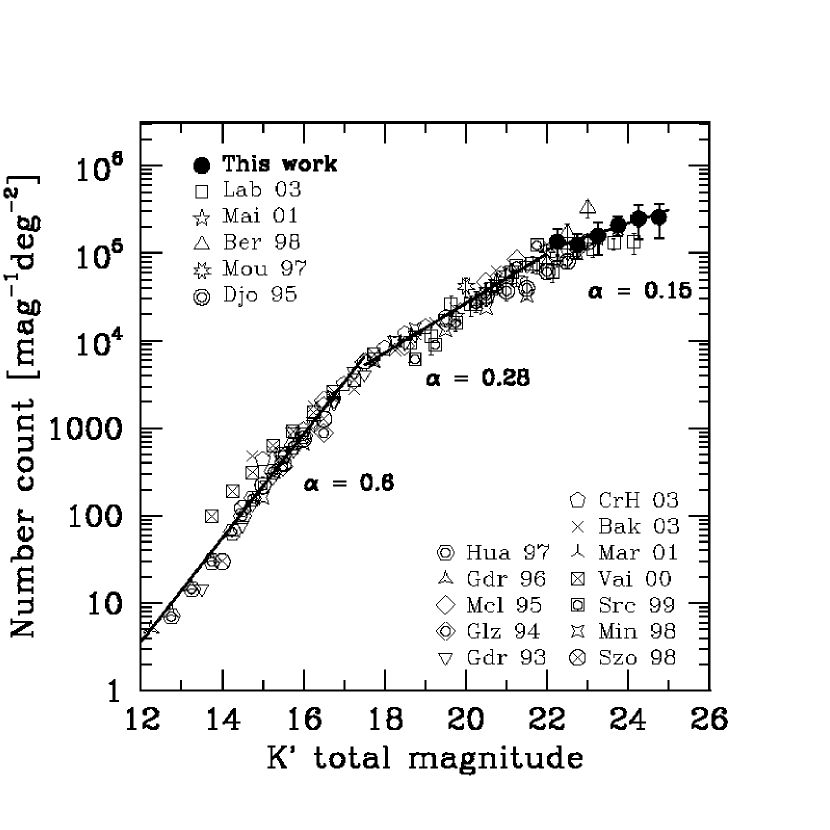
Figure 20.— Three power-law curves were fitted to the differential number counts of galaxies at $12<K^{\prime}<25$ based on the combined data of ours and those in the literatures. The count slope $\alpha=d\log N/dm$ is $0.59\pm 0.01$ at $K^{\prime}<17.5$, $0.29\pm 0.01$ at $17.5<K^{\prime}<22$, and $0.15\pm 0.08$ at $22<K^{\prime}<25$.

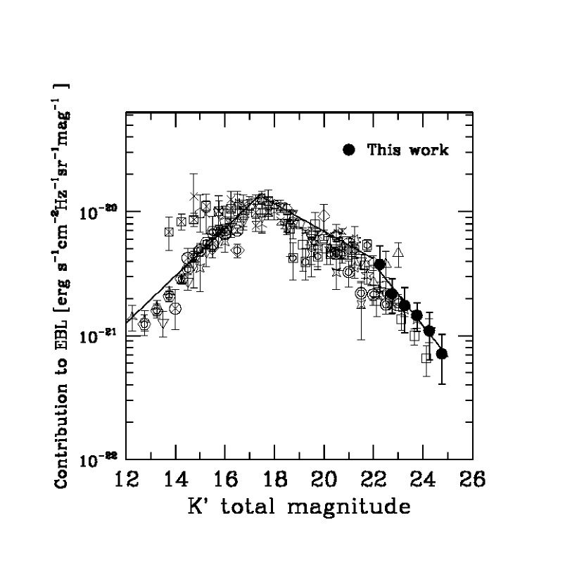
Figure 21.— Contributed flux of galaxies in each $K^{\prime}$-magnitude bin to the extragalactic background light (EBL). The data in the literatures are also shown using the same symbols as in Figure 20. Solid lines correspond to the fitted curves in Figure 20.

Based on our SSDF counts down to $K^{\prime}\sim 25$, which is 0.5 mag deeper than the SDF, we found that our estimated $K^{\prime}$-band EBL from galaxies is almost consistent with the theoretical estimation of Totani et al. (2001b). We also found that our estimated $K^{\prime}$-band EBL from galaxies is close to the $H$-band EBL from galaxies estimated from the HDF-N imaging (6$-$7 nWm^-2sr^-1, Thompson et al. 2001; Thompson 2003), which is comparable or even deeper than our $K^{\prime}$-band imaging. These results support the conclusion of Totani et al. (2001b) that the EBL from galaxies has been resolved almost completely into discrete sources of normal galaxies. Comparison of our estimated EBL from galaxies with the measurements of diffuse EBL in the $K$ band (20$-$29 nWm^-2sr^-1) shows that a population of galaxies accounts for only less than 50% of the diffuse EBL in the $K$ band. Unless the diffuse EBL measurements are contaminated by crucial systematic uncertainties, a population other than known galaxy populations at even fainter magnitude is necessary to explain such discrepancy. It has been pointed out that a hypothetical population might consist of population III stars at very high redshift, provided that a large amount of baryonic matter comparable to stars in galaxies should be used to form such exotic stars at extremely high rate (Santos et al., 2002; Salvaterra & Ferrara., 2003; Cooray & Yoshida, 2004).

7.3. Size distribution

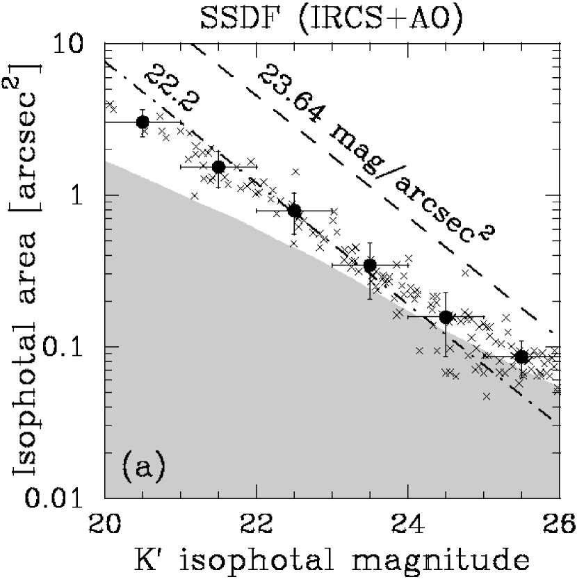
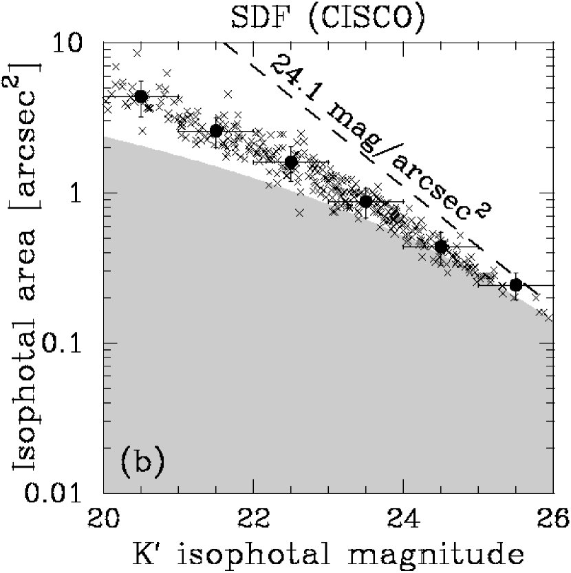
Figure 22.— Size distribution of the detected galaxies in the isophotal area versus isophotal magnitude diagram for (a) the SSDF and (b) the SDF. The SDF data were taken from Totani et al. (2001a). Crosses show the individual galaxies. Filled circles show the mean size in each one magnitude bin. The horizontal error bars show the bin size around the mean and the vertical error bars show the 1$\sigma$ dispersion of the isophotal area of the detected galaxies. The gray shaded region is where the isophotal area is less than the expected area of point source for each isophotal magnitude in the SSDF or the SDF. The dashed line shows the maximum isophotal area for each isophotal magnitude with the surface brightness (SB) threshold (23.64 mag/arcsec² for the SSDF, 24.1 mag/arcsec² for the SDF). Thanks to the high spatial resolution due to AO, we can resolve the galaxies having the area size of less than 0.1 arcsec² scale, which could not be done with the SDF image. The dot-dashed line in (a) shows the constant SB of 22.2 mag/arcsec². The constant SB line matches the observed size distribution within the uncertainty, although the observed size of the faint-end galaxies might be biased by the PSF. This suggests that the SB is not much different between high-redshift (faint) and low-redshift (bright) galaxies.

Figure 22 shows the size distribution of detected galaxies in the isophotal $K^{\prime}$-magnitude ($m_{iso}$) versus isophotal area ($A_{iso}$) diagram for the SSDF and the SDF. The observed mean size is shown by filled circles. The sizes of individual SDF galaxies (crosses in Figure 22b) are highly biased due to the large PSF size especially at faint magnitude of $K^{\prime}_{iso}>24$. However, because such bias is very small for the SSDF data thanks to the high spatial resolution with AO, the size of galaxies can be distinguished from that of PSF even in the faint end. The slope of $m_{iso}-A_{iso}$ relation in the SSDF seems to be constant at $20<K^{\prime}_{iso}<26$, yielding $d\log A_{iso}/dm_{iso}=-0.32\pm 0.12$. This slope is almost consistent with that of constant surface brightness ($d\log A_{iso}/dm_{iso}=-0.4$) within the uncertainties, while the slope in the SDF seems to be flatter in the faint end due to the large bias of the PSF. We note that the constant surface brightness of 22.2 mag/arcsec² (dot-dashed line in Figure 22a) matches the observed size distribution with the confidence level of 95%. This implies that the surface brightness is not much different between high-redshift (faint) and low-redshift (bright) galaxies.

Figure 23 compares the observed size distribution of galaxies to theoretical predictions from a standard model of pure luminosity evolution (PLE) of galaxies that assumes no number evolution or no merging of galaxies. We used the same model as Totani & Yoshii (2000) and Totani et al. (2001a), which is an updated version of Yoshii (1993). In this model, galaxies are divided into six morphological types (dE, gE, Sab, Sbc, Scd, Sdm) and their type-dependent luminosity evolutions are described by the model of Arimoto & Yoshii (1987) and Arimoto et al. (1992) in which the star formation history is determined to reproduce the present-day colors and chemical properties of galaxies. All galaxies are simply assumed to be formed at a single redshift of $z_{F}$=3. The surface brightness profiles of elliptical and spiral galaxies are modeled by the de Vaucouleurs and exponential profiles, respectively. These profiles are convolved with a moffat profile which nicely represents the observed PSF (see §6.2), and are used to calculate the isophotal area. The effective radius of galaxies is determined from the observed luminosity ($L$) versus effective radius ($r_{e}$) relation of local galaxies (Bender et al., 1992; Impey et al., 1996). Detailed descriptions of the model are given in Yoshii (1993), Totani & Yoshii (2000) and Totani et al. (2001a). The predicted $m_{iso}-A_{iso}$ relations for different types of galaxies are shown in Figure 23. We found that the predicted mean size for all types (thick solid line) is in good agreement with the observed mean size (filled circles).

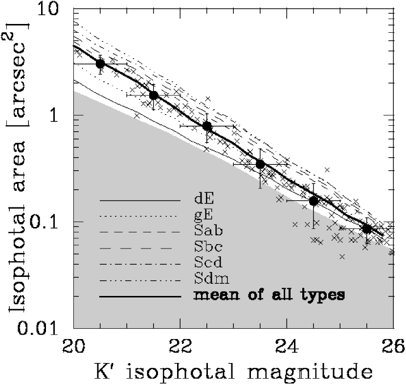
Figure 23.— Same figure in Figure 22(a), but with prediction of the PLE model with no size evolution described in the text. Thin lines show the predicted mean size for six morphological types of galaxies (dE, gE, Sab, Sbc, Scd, Sdm). The thick solid line shows the predicted mean size for all types of galaxies.

Figure 24 compares the observed size distribution to a PLE model that allows for intrinsic size evolution, in which galaxy size changes without changing the total luminosity (i.e. a size evolution is not driven by a number evolution). We here introduce a phenomenological parameter $\zeta$, and multiply an additional factor $(1+z)^{\zeta}$ to the size of PLE model galaxies used in Figure 23. It is seen from Figure 24 that the observed size distribution agrees with the model of $\zeta=0$, which favors no intrinsic size evolution, in agreement with the earlier claim by Yoshii (1993). This suggests that the $L-r_{e}$ relation of high-redshift galaxies is almost same as the local relation. Therefore, the result in Figure 22a that the surface brightness is not much different between high- and low-redshift galaxies is further strengthened.

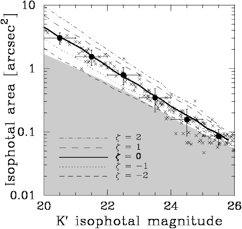
Figure 24.— Same figure as Figure 22(a), but with prediction of the PLE model which allows for size evolution, assuming that the effective radius of galaxies, $r_{e}$, evolves as $r_{e}\propto(1+z)^{\zeta}$. Solid line, which is identical to the thick solid line in Figure 23, shows the predicted mean size for all types of galaxies assuming no intrinsic size evolution ($\zeta=0$). The long-dashed, dot-dashed, dotted, and short-dashed lines show the models with size evolution of $\zeta$=1, 2, -1, and -2, respectively.

Totani et al. (2001a) performed the same analysis as ours using the SDF data taken by the Subaru/CISCO. They claimed that the size distribution of galaxies has the same trend as ours, although it was difficult to distinguish between the models of different types or different $\zeta$ based on their faint-end data at $K^{\prime}_{iso}\geq 24$, because the size of detected galaxies in the SDF was almost close to the size of PSF with FWHM $\sim$ 0$\farcs$45. For our SSDF data with AO, the PSF size is small enough to be separated from the galaxies at $K^{\prime}_{iso}\geq 24$, thereby confirming the claim by Totani et al. (2001a) unambiguously.

We note that a size evolution driven by a number evolution or merging is not necessarily ruled out if such process proceeds without changing the magnitude versus size relation in Figure 24. In fact, this relation is maintained if the typical surface brightness of galaxies is preserved by mergers. What we can conclude from our result is that the surface brightness of the faintest SSDF galaxies is not much different from that expected for a simple PLE model without size evolution. Therefore, our result places a strong constraint on the contemporary CDM-based structure formation theory (e.g., White & Rees 1978; Nagashima et al. 2002), in which galaxies are formed through merging of many smaller building blocks at different formation epochs. Further information can be obtained by the relation between redshift and effective radius of galaxies, which should be obtained from our SSDF data through the galaxy profile fitting (see Figure 13) and the photometric redshift technique (Minowa et al. 2005, in preparation).

8. Summary

We have presented the first result of deep $K^{\prime}$-band imaging of the SSDF with the Subaru AO. The achieved detection limit is $K^{\prime}\sim 24.7$ (5$\sigma$, 0$\farcs$2 aperture) for point source and $K^{\prime}\sim 23.5$ (5$\sigma$, 0$\farcs$6 aperture) for galaxies with the total integration time of 26.8 hours. The sensitivity gain due to the AO correction is about 0.5 mag. The achieved spatial resolution is 0$\farcs$18 in stellar FWHM on average. We found from the simulation that the extended wings of the observed AO PSF does not affect the measurement of the flux and size of the typical galaxies in the SSDF. Combination of high sensitivity and high spatial resolution by AO enables detailed morphological study of high-redshift galaxies with the profile fitting technique. From a similar AO observation of globular cluster M13, we confirmed that the variation of the spatial resolution and the sensitivity to the point source (anisoplanatism) is not significant within our 1′$\times$ 1′ field of view.

The slope of differential galaxy number counts ($\alpha\equiv d\log N/dm$) is about 0.15 at $22<K^{\prime}<25$. Our count slope is consistent with that of the HDF-S (FIRES, Labbe et al., 2003), in which the slope changes from $\alpha\simeq 0.25$ at $20<K^{\prime}<22$ to $\alpha\simeq 0.15$ at $22<K^{\prime}<24$. Thus, our data support the flatter slope of $\alpha\simeq 0.15$ at $K^{\prime}>22$ with the deepest image to date, while the other $K$-band deep surveys show the steeper slope at the faint-end. The discrepancies of faint-end counts between ours and other surveys might be caused by either field-to-field variation or different technique of incompleteness correction.

The contributed flux of galaxies to the EBL is about 9.43 nWm^-2sr^-1, and 98% of which appears to be resolved into discrete galaxies in the SSDF at $K^{\prime}<25$. However, our EBL estimate can account for only less than 50% of the total flux of diffuse EBL which was independently measured by satellites in the similar $K$ band. Our result further strengthens the previous claim by Totani et al. (2001b) that there must be an exotic population that significantly contributes to the EBL, unless the measurements of diffuse EBL are contaminated by crucial systematic uncertainties.

We examined the size distribution of galaxies in the isophotal magnitude versus isophotal area diagram. In this diagram, the size distribution of detected galaxies was obtained down to the area size of less than 0.1 arcsec², which is less than a half of that of the previous SDF galaxies. We found that the relation of observed mean size as a function of magnitude is nicely explained by a simple PLE model. We examined a possibility of intrinsic size evolution using a PLE model that allows for size evolution, and found that the model with no size evolution gives the best fit to the data. We conclude that the surface brightness of galaxies at high redshift is not much different from that expected from the size-luminosity relation of present-day galaxies. We cannot rule out a size evolution associated with a number evolution of galaxies if their surface brightness is preserved. In other words, our result of constant surface brightness should place a strong constraint on the merging process in a hierarchical structure formation theory.

References

- Arimoto & Yoshii (1987) Arimoto, N., & Yoshii, Y. 1987, A&A, 173, 23
- Arimoto et al. (1992) Arimoto, N., Yoshii, Y., & Takahara, F. 1992, A&A, 253, 21
- Babul & Ferguson (1996) Babul, A. & Ferguson, H. C. 1996, ApJ, 458, 100
- Baker et al. (2003) Baker, A. J. et al. 2003, A&A, 406, 593
- Baugh et al. (1996) Baugh, C. M., Gardner, J. P., Frenk, C. S., & Sharples, R. M. 1996, MNRAS, 283, L15
- Bernstein et al. (2002) Bernstein, R. A., Freedman, W. L., & Madore, B. F. 2002, ApJ, 571, 107
- Bershady et al. (1998) Bershady, M. A., Lowenthal, J. D., & Koo, D. C. 1998, ApJ, 505, 50
- Bender et al. (1992) Bender, R., Burstein, D., & Faber, S. M. 1992, ApJ, 399, 462
- Bertin & Arnouts (1996) Bertin, E & Arnouts, S 1996, A&AS, 117, 393
- Bond et al. (1986) Bond, J. R., Carr, B. J., & Hogan, C. J. 1986, ApJ, 306, 428
- Cambrésy et al. (2001) Cambrésy, L., Reach, W. T., Beichman, C. A., & Jarrett, T. H. 2001, ApJ, 555, 563
- Carlberg et al. (1997) Carlberg, R. G., Cowie, L. L., Songaila, A., & Hu, E. M. 1997, ApJ, 484, 538
- Cooray & Yoshida (2004) Cooray, A. & Yoshida, N. 2004, MNRAS, 351, 71
- Cristóbal-Hornillos et al. (2003) Cristóbal-Hornillos, D., Balcells, M., Prieto, M., Guzmán, R., Gallego, J., Cardiel, N., Serrano, Á., & Pelló, R. 2003, ApJ, 595, 71
- de Vaucouleurs (1948) de Vaucouleurs, G. 1948, Annales d’Astrophysique, 11, 247
- Djorgovski et al. (1995) Djorgovski, S. et al. 1995 ApJ, 438, 13
- Freeman (1970) Freeman, K. C. 1970, ApJ, 160, 811
- Fugal & Moody (2003) Fugal, J. P., & Moody, J. W. 2003, PASP, 115, 295
- Gardner et al. (1993) Gardner, J. P., Cowie, L. L., & Wainscoat, R. J. 1993, ApJ, 415, L9
- Gardner et al. (1996) Gardner, J. P., Sharples, R. M., Carrasco, B. E., & Frenk, C. S. 1996, MNRAS, 282, L1
- Gardner et al. (2000) Gardner, J. P., et al. 2000, AJ, 119, 486
- Glazebrook et al. (1994) Glazebrook, K., Peacock, J. A., Miller, L., & Collins, C. A. 1994, MNRAS, 266, 65
- Gorjian et al. (2000) Gorjian, V., Wright, E. L., Chary, R. R. 2000, ApJ, 536, 550
- Groth & Peebles (1977) Groth E. J., Peebles P. J. E. 1977, ApJ217, 38
- Hardy (1998) Hardy, J. W. 1998, Adaptive Optics for Astronomical Telescopes (New York: Oxford University Press)
- Huang et al. (1997) Huang, J. S., Cowie, L. L., Gardner, J. P., Hu, E. M., Songaila, A., & Wainscoat, R. J. 1997, ApJ, 476, 12
- Impey et al. (1996) Impey, C. D., Sprayberry, D., Irwin, M. J., & Bothun, G. D. 1996, ApJS, 105, 209
- Iye et al. (2004) Iye, M. et al. 2004, PASJ, 56, 381
- Kahikawa et al. (2004) Kashikawa, N. et al. 2004, PASJ, 56, 1011
- Kajisawa & Yamada (2001) Kajisawa, M. & Yamada, T. PASJ, 53, 833
- Kobayashi et al. (2000) Kobayashi, N. et al. 2000 Proc. SPIE, 4008, 1506
- Labbe et al. (2003) Labbe, I. et al. 2003 AJ, 125, 1107
- Madau & Pozzetti (2000) Madau, P. & Pozzetti, L. 2000, MNRAS, 312, L9
- Maihara et al. (2001) Maihara, T. et al. 2001 PASJ53, 25
- Martini (2001) Martini, P. 2001, AJ, 121, 598
- Matsumoto et al. (2001) Matsumoto, T., et al. 2001, in ISO Surveys of a Dusty Universe, ed. D. Lemke, M. Stickel, & K. Wilke (New York: Springer)
- Mcleod et al. (1995) McLeod, B. A., Bernstein, G. M., Rieke, M. J., Tollestrup, E. V., & Fazio, G. G. 1995, ApJS, 96, 117
- Minezaki et al. (1998a) Minezaki, T., Kobayashi, Y., Yoshii Y., & Peterson B. A. 1998 ApJ, 494, 111
- Minezaki et al. (1998b) Minezaki, T., Yoshii, Y., Cohen, M., Kobayashi, Y., Peterson, B. A. 1998, AJ, 115, 229
- Miyazaki et al. (2002) Miyazaki, S. et al. 2002 PASJ, 54, 833
- Motohara et al. (2002) Motohara, K. et al. 2002 PASJ, 54, 315
- Moustakas et al. (1997) Moustakas, L. A., Davis, M., Graham, J. R., Silk, J., Peterson, B. A., & Yoshii, Y. 1997, ApJ, 475, 445
- Nagashima et al. (2002) Nagashima, M., Yoshii, Y., Totani, T., & Gouda, N. 2002, ApJ, 578, 675
- Persson et al. (1998) Persson S. E., Murphy, D. C., Krzeminski, W., Roth, M., & Rieke, M. J. 1998, AJ, 116, 2475
- Roche & Eales (1999) Roche, N. & Eales, S. A. 1999, MNRAS, 307, 703
- Roche et al. (1999) Roche, N., Eales, S. A., Hippelein, H., & Willott, C. J. 1999, MNRAS, 306, 538
- Salvaterra & Ferrara. (2003) Salvaterra, R. & Ferrara, A. 2003, MNRAS, 339, 973
- Santos et al. (2002) Santos, M. R., Bromm, V., & Kamionkowski, M. 2002, MNRAS, 336, 1082
- Saracco et al. (1999) Saracco, P., D’Odorico, S., Moorwood, A., Buzzoni, A., Cuby, J.-G., & Lidman, C. 1999, A&A, 349
- Sheth et al. (2003) Sheth, K., Regan, M. W., Scoville, N. Z., & Strubbe, L. E. 2003, ApJ, 592, L13
- Smail et al. (1995) Smail, I., Hogg, D. W., Yan, L., & Cohen, J. G. 1995, ApJ, 449, 105
- Szokoly et al. (1998) Szokoly, G., Subbarao, M., Connoly, A., & Mobasher, B. 1998, ApJ, 492, 452
- Takami et al. (2004) Takami, H. et al. 2004 PASJ, 56, 225
- Thompson (2003) Thompson, R. I. 2003 ApJ, 596, 748
- Thompson et al. (2001) Thompson, R. I., Weymann, R. J., & Storrie-Lombardi, L. J. 2001, ApJ, 546, 694
- Tokunaga et al. (1998) Tokunaga, A. T. et al. 1998 Proc. SPIE, 3354, 512
- Tokunaga et al. (2002) Tokunaga, A. T., Simons, D. A., & Vacca, W. D. 2002, PASP, 114, 180
- Tomita (1995) Tomita, K. 1995, ApJ, 451, 1
- Totani & Yoshii (2000) Totani, T. and Yoshii, Y. 2000, ApJ, 540, 81
- Totani et al. (2001a) Totani, T., Yoshii, Y., Maihara, T., Iwamuro, F., & Motohara, K. 2001 ApJ, 559, 592
- Totani et al. (2001b) Totani, T., Yoshii, Y., Maihara, T., Iwamuro, F., & Motohara, K. 2001 ApJ, 550, 137
- Väisänen et al. (2000) Väisänen, P., Tollestrup, E. V., Willner, S. P., & Cohen, M. 2000, ApJ, 540, 593
- White & Rees (1978) White, S. D. M. & Rees, M. J. 1978, MNRAS, 183, 341
- Williams et al. (1996) Williams, R. T., et al. 1996, AJ, 112, 1335
- Williams et al. (2000) Williams, R. T., et al. 2000, AJ, 120, 2735
- Wright (2001) Wright, E. L. 2001, ApJ, 553, 538
- Yan et al. (1998) Yan, L., McCarthy, P. J., Storrie-Lombardi, L. J., & Weymann, R. J. 1998, ApJ, 503, 19
- Yoshii & Takahara (1988) Yoshii, Y. & Takahara, F. 1988, ApJ, 326, 1
- Yoshii (1993) Yoshii, Y. 1993, ApJ, 403, 552