astro-ph/0505339

TU-744

May 2005

Implications of the Curvaton on Inflationary Cosmology

Takeo Moroi^a and Tomo Takahashi^b

^aDepartment of Physics, Tohoku University
Sendai 980-8587, Japan

^bInstitute for Cosmic Ray Research, University of Tokyo
Kashiwa 277-8582, Japan

We study implications of the curvaton, a late-decaying light scalar field, on inflationary cosmology, paying particular attentions to modifications of observable quantities such as the scalar spectral index of the primordial power spectrum and the tensor-to-scalar ratio. We consider this issue from a general viewpoint and discuss how the observable quantities are affected by the existence of the curvaton. It is shown that the modification owing to the curvaton depends on class of inflation models. We also study the effects of the curvaton on inflation models generated by the inflationary flow equation.

1 Introduction

Recent precise observations of the cosmic microwave background (CMB) radiation [1] and the large scale structure [2] have provided deep insights into the origin of the cosmic density fluctuations. In particular, it has become clear that the primordial density fluctuation is almost scale invariant. As a mechanism to generate the scale invariant density fluctuation, inflation [3] is the most prominent candidate.

Even with inflation, however, it is not automatic to make the present density fluctuations to be consistent with the observational constraints. In the standard scenario, fluctuation of the inflaton field, whose potential energy is responsible for the energy density during the inflation, is generated during the inflation and it becomes the origin of the present density fluctuations. In this case, properties of the present density fluctuations are determined once the inflaton potential is fixed, and we obtain constraints on the individual inflation models.

If there exists some scalar field other than the inflaton, however, the mechanism of generating the cosmic density fluctuations may become more complicated. In particular, with a scalar field whose mass is much smaller than the expansion rate during the inflation, fluctuation is imprinted in the amplitude of such scalar field, which provides another potential source of the present density fluctuations. In this paper, we consider one of such examples, the curvaton [4]. In the curvaton scenario, there exists a late-decaying scalar condensation (the curvaton) which acquires amplitude fluctuation during the inflation. When the curvaton decays, fluctuation of the curvaton amplitude becomes the fluctuation of the radiation (and of other components in the universe). Thus, if the curvaton exists, properties of the present density fluctuations change compared to the standard scenario only with the inflaton. From the particle physics point of view, there are various well-motivated candidates of the curvaton [7].

Since the recent results from Wilkinson microwave background probe (WMAP) [1] provided severe constraints on the properties of the primordial density fluctuations, it is interesting to reconsider the observational constraints in the framework of the curvaton scenario. With the curvaton, it is expected that the constraints on the inflation models are changed (and possibly relaxed) compared with the case without the curvaton.

Indeed, in the past, it was pointed out that the constraints on the scale of the inflation is drastically relaxed with the curvaton [8]. Then, there have been subsequent works focusing on the low scale inflation in the curvaton scenario [9, 10, 11, 12]. Furthermore, in Ref. [13], the authors has shown that the quartic chaotic inflation model, which is marginally excluded by WMAP observations, becomes viable when the curvaton mechanism applies. In Ref. [14], several other inflation models were investigated such as chaotic inflation with several monomials, the natural inflation model and the new inflation model. The discussions made in Refs. [13, 14] are mainly based on the scalar spectral index and the tensor-to-scalar ratio. Importantly, although some inflation models can become viable with the curvaton even if they are excluded by current observations, there exist other class of models which cannot be liberated even with the curvaton. In particular, in Ref. [14], it was discussed how the liberation of inflation models depends on model parameters such as the initial amplitude, mass and decay rate of the curvaton field.

In this paper, we discuss the implication of the curvaton on inflation models from some general points of view. In the previous works, the analysis have been rather dependent on inflaton potentials. Of course, it is important to study individual inflation models motivated from, in particular, particle physics point of view. It is, however, also possible to adopt some other approach, parameterizing the inflation models by using the slow-roll parameters (at some epoch during the inflation). In this approach, one generates inflation models with some stochastic method such as using the inflationary flow equations [15, 16]. Such a method has been used in many studies including the one by the WMAP team and constraints on inflation models have been discussed [17, 18, 19, 20, 21, 22]. Although other approaches such as stochastic approaches or implementations of the flow equation are proposed [23], we discuss the implications of the curvaton on inflation models generated by the usual flow equation as an example.

The organization of this paper is as follows. In the next section, we start with briefly reviewing the formalism to study how observable quantities are affected in the system containing the inflaton and the curvaton. We discuss how the standard scenario is modified in terms of the background evolution and the perturbation. We also review the classification of single-field inflation models. After the preparation, in section 3, we go into how observational quantities are affected by introducing the curvaton and discuss it from some general viewpoints. In section 4, we consider the effects of the curvaton on inflation models generated by the inflationary flow equation. Then we conclude this note by summarizing the results in the final section.

2 Formalism

2.1 Background evolution

First we present the background evolution in the curvaton scenario comparing its counterpart of the standard case.

In the standard case, the potential energy of the inflaton drives the inflation. During inflation, the inflaton slowly rolls down the potential. However, at some point, the inflaton starts to roll fast down the potential hill, then the inflaton begins to oscillate around the minimum of the potential. When the potential of the inflaton can be approximated by the quadratic form as $V(\chi)\sim(1/2)m_{\chi}^{2}\chi^{2}$, the energy density of the inflaton behaves as matter component. Then the universe is dominated by the oscillating inflaton. We call this epoch “$\chi$ dominated” or “$\chi$D.” After some time, when the expansion rate of the universe, namely the Hubble parameter, becomes as the same as the decay rate of the inflaton, the inflaton decays into radiation. Then the universe becomes radiation dominated. This is, what we call, the standard thermal history of the universe.

When the curvaton exists, above picture is modified. First we consider the case where the initial amplitude of the curvaton is so small that the potential energy of the curvaton does not drive the (second) inflation. During inflation, the curvaton field stays at somewhere on the potential. If we adopt the potential of the curvaton to be of the form $V(\phi)\sim(1/2)m_{\phi}^{2}\phi^{2}$, the curvaton begins to oscillate around the minimum of the potential when the Hubble parameter becomes of the same order of the mass of the curvaton. During this epoch, the energy density of the curvaton behaves as ordinary matter. This event usually happens when the universe is dominated by radiation which comes from the decay of the inflaton. Since the energy density of matter decreases slower than that of radiation, at some point, the energy density of the curvaton becomes to dominate the universe. We call this epoch as $\phi$ dominated or $\phi$D. After some time, the curvaton also decays into radiation when the expansion rate of the universe becomes of the same order as the decay rate of the curvaton. Then the universe becomes radiation dominated again. We call this epoch as RD2 not to confuse with the radiation dominated epoch from the inflaton decay. (We call the first radiation dominated epoch as RD1.)

Next we discuss the case where the energy density of the curvaton can drive the second inflation after the first one induced by the inflaton. When the initial amplitude of the curvaton is large enough, the second inflation can happen after the $\chi$D or RD1 epoch before $\phi$ starts to oscillate. In this case, the universe experiences the inflation era driven by the inflaton, $\chi$D era, RD1 era and the second inflation driven by the curvaton potential energy, followed by the $\phi$D era and RD2 era. The second inflation can modify the observable quantities drastically in some cases. We discuss this point later.

2.2 Density perturbations: Standard case

Now we briefly review the issue of density perturbation in the standard case.

To discuss observational consequences, we have to set up the initial condition during radiation dominated era after the decay of the inflaton. For this purpose, we represent the primordial power spectrum with the (Bardeen’s) gravitational potential $\Phi$ which appears in the perturbed metric in the conformal Newtonian (or longitudinal) gauge as

$$ds^{2}=-a^{2}(1+2\Phi)d\tau^{2}+a^{2}(1-2\Psi)dx^{2},$$ (2.1)

with $\tau$ being the conformal time. The quantum fluctuation of the inflaton $\delta\chi$ during inflation generates the curvature perturbation as $\mathcal{R}=-(H/\dot{\chi})\delta\chi$. Since $\delta\chi\simeq H/2\pi$ and, $\Phi$ and $\mathcal{R}$ are related as $\Phi=-(2/3)\mathcal{R}$ during radiation-dominated era, the power spectrum of the curvature perturbation from the inflaton fluctuation is [24]

$$P_{\Phi}^{\rm(inf)}=\left[1-2(1+3C)\epsilon_{V}+2C\eta_{V}\right]\frac{1}{12\pi^{2}M_{\rm pl}^{6}}\frac{V_{\rm inf}^{3}}{V_{\rm inf}^{{}^{\prime}2}}\biggr{|}_{k=aH},$$ (2.2)

where the “prime” represents the derivative with respect to $\chi$ and $C=-2+\ln 2+\gamma$, with $\gamma\simeq 0.577$ being the Euler’s constant. Here, we used the “potential” slow-roll parameters. There are two ways to define the slow-roll parameters: one is the one using inflaton potential and the other is the one using the Hubble parameter. The “potential” slow-roll parameters are defined as

$$\epsilon_{V}\equiv\frac{1}{2}M_{\rm pl}^{2}\left(\frac{V_{\rm inf}^{\prime}}{V_{\rm inf}}\right)^{2},~{}~{}~{}\eta_{V}\equiv M_{\rm pl}^{2}\frac{V_{\rm inf}^{\prime\prime}}{V_{\rm inf}},~{}~{}~{}\xi^{2}_{V}\equiv M_{\rm pl}^{2}\frac{V^{\prime}_{\rm inf}{V^{{}^{\prime\prime\prime}}_{\rm inf}}}{V_{\rm inf}^{2}}.$$ (2.3)

where the third parameter $\xi^{2}_{V}$ is considered to be the second order in the slow-roll.

The “Hubble” slow-roll parameters are defined as

$$\epsilon_{H} \equiv 2M_{\rm pl}^{2}\left(\frac{H^{\prime}}{H}\right)^{2}=\epsilon_{V},$$

$$\eta_{H} \equiv 2M_{\rm pl}^{2}\frac{H^{{}^{\prime\prime}}}{H}=-\epsilon_{V}+\eta_{V},$$

$$\xi^{2}_{H} \equiv 2M_{\rm pl}^{4}\frac{H^{\prime}H^{{}^{\prime\prime\prime}}}{H^{2}}=\xi_{V}^{2}-3\epsilon_{V}\eta_{V}+3\epsilon_{V}^{2}$$ (2.4)

where we also write the relation between the Hubble and potential slow-roll parameters to the first order in slow-roll.

The scalar spectral index is defined as

$$n_{s}-1\equiv\frac{d\ln P_{\Phi}}{d\ln k}.$$ (2.5)

Using the slow-roll parameters, the spectral index can be written as

$$n_{s}^{\rm(inf)}-1=-6\epsilon_{V}+2\eta_{V}-2(7+12C)\epsilon_{V}^{2}+2(3+8C)\epsilon_{V}\eta_{V}-2C\xi_{V}^{2},$$ (2.6)

where “(inf) ” represents that the expression of $n_{s}$ is for the case where primordial fluctuation comes from the fluctuation of the inflaton.

In the second order, we have the running of the scalar spectral index which is

$$\frac{d\ln n^{\rm(inf)}_{s}}{d\ln k}=-24\epsilon_{V}^{2}+16\epsilon_{V}\eta_{V}-2\xi_{V}^{2}.$$ (2.7)

During inflation, the gravity wave can also be generated. The primordial gravity wave (tensor) power spectrum is given by

$$P_{T}^{\rm(inf)}=\frac{2V_{\rm inf}}{3\pi^{2}M_{\rm pl}^{4}}.$$ (2.8)

With this expression, the tensor-to-scalar ratio $r$ is defined and given by

$$r^{\rm(inf)}\equiv\frac{P_{T}^{\rm(inf)}}{P_{\mathcal{R}}^{\rm(inf)}}=\frac{4}{9}\frac{P_{T}^{\rm(inf)}}{P_{\Phi}^{\rm(inf)}}=16\epsilon_{V}\left(1+4C\epsilon_{V}-2C\eta_{V}\right).$$ (2.9)

2.3 A classification of inflation models

Here we discuss one of possible classifications of single-field inflation models. In many literatures, the following classification has been used; single-field inflation models can be classified into the “small-field,” “ large-field” and “hybrid-type” models [25]. In this classification, the models are classified on the $n_{s}-r$ plane and distinguished by the value of the slow-roll parameters or the first and second derivatives of the inflaton potential. To the first order in the slow-roll parameters, the observational plane $(n_{s},r)$ is uniquely divided into the three classes. In this section, we consider the slow-roll approximation in the first order.

The “small-field” models are identified with the condition $V^{\prime\prime}(\chi)<0$ and $(V^{\prime}/V)^{2}>V^{\prime\prime}/V$, which also means $2\epsilon_{V}>0>\eta_{V}$. This category includes, for example, the new and natural inflations. The generic potential of this type is

$$V(\chi)=\lambda v^{4}\left[1-\left(\frac{\chi}{v}\right)^{p}\right].$$ (2.10)

The scalar spectral index and the tensor-to-scalar ratio of this type of model can be written with the slow-roll parameter defined in Eq. (2.3) and the number of $e$-foldings during inflation which is defined as $N_{e}\equiv\ln(a_{\rm end}/a_{*})$ where $a_{\rm end}$ and $a_{*}$ are the scale factor at the end of inflation and the time of horizon crossing. Using the slow-roll approximation, $N_{e}$ is given by

$$N_{e}=\frac{1}{M_{\rm pl}^{2}}\int_{\chi_{\rm end}}^{\chi_{*}}\frac{V_{\rm inf}}{V^{\prime}_{\rm inf}}d\chi.$$ (2.11)

Using the $e$-folding number $N_{e}$, the slow-roll parameters for this type of model are given by, for $p>2$,

$$\epsilon_{V} = \frac{p^{2}}{2}\left(\frac{M_{\rm pl}}{v}\right)^{2}\left[\frac{1}{p(p-1)N_{e}}\left(\frac{v}{M_{\rm pl}}\right)^{2}\right]^{\frac{2(p-1)}{p-2}},$$ (2.12)

$$\eta_{V} = -\frac{p-1}{p-2}\frac{1}{N_{e}}$$ (2.13)

For $v<M_{\rm pl}$, the $\epsilon$ parameter becomes very small, thus the spectral index is given by

$$n_{s}^{\rm(inf)}-1=-2\frac{p-1}{p-2}\frac{1}{N_{e}}$$ (2.14)

The “large-field models” are identified with the condition $V^{\prime\prime}(\chi)>0$ and $(V^{\prime}/V)^{2}>V^{\prime\prime}/V$, which also means $2\epsilon_{V}>\eta_{V}>0$. This category includes, for example, the chaotic inflation. The generic potential of this type is

$$V(\chi)=\lambda M_{\rm pl}^{4}\left(\frac{\chi}{M_{\rm pl}}\right)^{\alpha}.$$ (2.15)

The $n_{s}$ and $r$ are obtained as similarly as the case with the small-field models as

$$n_{s}^{\rm(inf)}-1 = -\frac{\alpha+2}{2N_{e}},$$ (2.16)

$$r^{\rm(inf)} = \frac{4\alpha}{N_{e}}.$$ (2.17)

Thus inflation models in this category predict red-tilted scalar primordial spectrum and relatively large tensor-to-scalar ratio.

The final one, “hybrid-type” models are identified with the condition $V^{\prime\prime}(\chi)>0$ and $(V^{\prime}/V)^{2}<V^{\prime\prime}/V$, which implies $2\epsilon_{V}<\eta_{V}$. This category includes, the hybrid inflation model as the name tells. Only models of this category can give blue-tilted spectrum.

2.4 Effects of the curvaton fluctuation

Here we briefly review the effects of the fluctuation of the curvaton on the observable quantities such as $n_{s}$ and $r$. (For details, see [13, 14, 26].) For the case where the fluctuations of the inflaton and the curvaton both affect the cosmic density perturbation today, the gravitational potential during RD2 era is given by

$$\Phi_{\rm RD2}=-\left[1-(1+3C)\epsilon_{V}+C\eta_{V}\right]\frac{2}{3M_{\rm pl}^{2}}\frac{V_{\rm inf}}{V_{\rm inf}^{\prime}}\delta\chi_{\rm init}-f(X)\frac{\delta\phi_{\rm init}}{M_{\rm pl}},$$ (2.18)

where $\delta\phi_{\rm init}$ is the primordial fluctuation of the curvaton, and

$$X=\frac{\phi_{\rm init}}{M_{\rm pl}}.$$ (2.19)

The function $f(X)$ represents the size of the contribution from the fluctuation of the curvaton. $f(X)$ can be calculated using the linear perturbation theory [13]. Assuming that the curvaton dominates the universe once in the course of the history of the universe, $f(X)$ can be given, for small and large $X$, by

$$f(X)\simeq\left\{\begin{array}[]{ll}\displaystyle{\frac{4}{9X}}&~{}~{}~{}:~{}~{}~{}\phi_{\rm init}\ll M_{\rm pl}\\ \\ \displaystyle{\frac{1}{3}X}&~{}~{}~{}:~{}~{}~{}\phi_{\rm init}\gg M_{\rm pl}\end{array}\right..$$ (2.23)

Using Eq. (2.18), the scalar spectral index can be written as

$$P_{\Phi}=\left[1+\tilde{f}^{2}(X)\epsilon_{V}-2(1+3C)\epsilon_{V}+2C\eta_{V}\right]\frac{V_{\rm inf}}{54\pi^{2}M_{\rm pl}^{4}\epsilon_{V}},$$ (2.24)

where $\tilde{f}=(3/\sqrt{2})f$. Thus the scalar spectral index is given by using Eq. (2.6)

$$n_{s}-1=-2\epsilon_{V}+\frac{2\eta_{V}-4\epsilon_{V}}{1+\tilde{f}^{2}\epsilon_{V}}-2(7+12C)\epsilon_{V}^{2}+2(3+8C)\epsilon_{V}\eta_{V}-2C\xi^{2}_{V}$$ (2.25)

The running of the scalar spectral index is given by

$$\frac{d\ln n_{s}}{d\ln k}=4\epsilon_{V}(\eta_{V}-2\epsilon_{V})-\frac{16\epsilon^{2}_{V}-12\epsilon_{V}\eta_{V}+2\xi_{V}^{2}}{1+\tilde{f}^{2}\epsilon_{V}}+\frac{4\tilde{f}^{2}\epsilon_{V}(\eta_{V}-2\epsilon_{V})^{2}}{(1+\tilde{f}^{2}\epsilon_{V})^{2}}.$$ (2.26)

The tensor power spectrum is not modified even with the curvaton. However, since the scalar perturbation spectrum is modified, the tensor-to-scalar ratio becomes

$$r=\frac{16\epsilon}{1+\tilde{f}^{2}\epsilon}(1+4C\epsilon_{V}-2C\eta_{V}).$$ (2.27)

2.5 Effects of modification of the background evolution

Here we discuss effects of the modification of the background evolution due to the curvaton. Generally, the observable quantities such as the scalar spectral index and the tensor-to-scalar ratio depends on the field value of the inflaton at the time of horizon crossing which can usually be expressed with the number of $e$-foldings during inflation. The fluctuation which corresponds to some reference scale $k_{\rm ref}$ at present epoch can be approximately given, in the standard case, as [27]

$$\frac{k_{\rm ref}}{a_{0}H_{0}}=\frac{a_{k}H_{k}}{a_{0}H_{0}}=e^{-N_{e}(k)}\frac{a_{\rm end}}{a_{\rm reh}}\frac{a_{\rm reh}}{a_{0}}\frac{H_{k}}{H_{0}}$$ (2.28)

where “end” and “reh” denote the time when the inflation ends and the reheating epoch, i.e., the beginning of RD epoch. Thus the $e$-folding number during inflation is given by

$$N_{e}(k)^{\rm(standard)}\simeq-\ln\frac{k}{a_{0}H_{0}}-\frac{n+2}{6n}\ln\frac{\rho_{\rm end}}{\rho_{\rm reh}}+\frac{1}{3}\ln\frac{s_{0}}{s_{\rm reh}}+\ln\frac{H_{\rm inf}}{H_{0}}$$ (2.29)

where we assumed that the energy density of the oscillating inflaton behaves as $\rho_{\chi}\propto a^{-6n/(n+2)}$ which corresponds to the case with inflaton potential $V_{\rm inf}\propto\chi^{n}$. $s_{\rm reh}$ and $s_{0}$ are the entropy density at present time and time of reheating, respectively. In the last term, we assumed that the Hubble parameter is almost constant during inflation, thus we replaced $H_{k}$ with $H_{\rm inf}$. Notice that the decay rate of the inflaton $\Gamma_{\chi}$ and parameters in the potential are needed to determine $N_{e}$ exactly. Depending on $\Gamma_{\chi}$ and the parameters in the potential, the number of $e$-folding can be changed as

$$N_{e}\simeq\frac{4-\alpha}{6\alpha}\ln\Gamma_{\chi}+\cdots$$ (2.30)

Now we discuss the $e$-folding number in the curvaton scenario. When the curvaton is introduced, Eq. (2.28) is modified as

$$\frac{k_{\rm ref}}{a_{0}H_{0}}=e^{-N_{e}(k)^{\rm(curvaton)}}\frac{a_{\rm end}}{a_{\rm reh1}}\frac{a_{\rm reh1}}{a_{\rm inf2}}\frac{a_{\rm inf2}}{a_{\phi\rm D}}\frac{a_{\phi\rm D}}{a_{\rm reh2}}\frac{a_{\rm reh2}}{a_{0}}\frac{H_{k}}{H_{0}}$$ (2.31)

where “reh1,” “inf2,” “$\phi$D2,” and “reh2” denote the time when the first radiation dominated epoch begins, the second inflation begins, the oscillating curvaton dominated begins and the second radiation dominated epoch begins, respectively. When the initial amplitude of the curvaton is small ($\phi_{\rm init}\ll M_{\rm pl}$), there is no second inflation. In that case, $(a_{\rm reh1}/a_{\rm inf2})(a_{\rm inf2}/a_{\phi\rm D})$ should be replaced with $(a_{\rm reh1}/a_{\phi\rm D})$.

Assuming that the curvaton field does not dominate the energy density of the universe when the curvaton begins to oscillate, namely the case with no second inflation driven by the curvaton, we get [28].

$$N_{e}(k)^{\rm(curvaton)} \simeq N_{e}(k)^{\rm(standard)}-\frac{1}{12}\ln\frac{\rho_{\phi\rm D}}{\rho_{\rm reh2}}$$ (2.32)

$$\simeq N_{e}(k)^{\rm(standard)}-\frac{1}{6}\ln\frac{m_{\phi}}{\Gamma_{\phi}}-\frac{2}{3}\ln\frac{\phi_{\rm init}}{M_{\rm pl}}$$

In Fig. 1, we plot contours of constant $\Delta N_{e}\equiv N_{e}^{\rm(curvaton)}-N_{e}^{\rm(standard)}$ in the $m_{\phi}/\Gamma_{\phi}$ vs. $X$ plane. Requiring that the curvaton dominates the energy density of the universe after the first radiation dominated epoch, i.e., $\rho_{\phi}>\rho_{\rm rad}$ at the time when the curvaton decays into radiation, we have the relation among the mass, the decay rate and the initial amplitude of the curvaton as

$$\frac{m_{\phi}}{\Gamma_{\phi}}>\frac{1}{9}X^{4}.$$ (2.33)

In Fig. 1, the region where the above inequality is not satisfied is represented with small circles.

Figure 1: Contours of constant $\Delta N_{e}$ in the $m_{\phi}/\Gamma_{\phi}$ vs. $X$ plane. The region where the curvaton does not dominate the universe is represented with small circles.

As seen from Eqs. (2.14) and (2.16), the scalar spectral index in the small-field and large-field models are inversely proportional to $N_{e}$. Thus slight change of $N_{e}$ affects $n_{s}^{\rm(inf)}$ as $|\Delta n_{s}^{\rm(inf)}|\sim\Delta N_{e}/N_{e}^{2}$. This implies that, requiring $|\Delta n_{s}^{\rm(inf)}|<0.001$, $\Delta N_{e}<4-5$ for $N_{e}=50-60.$ Notice that the uncertainty of the $e$-folding number $N_{e}$ also comes from the inflaton sector through the decay rate of the inflaton and the form of the potential, in particular around the minimum (i.e., the potential which the inflaton feels when the inflaton oscillates.)

When the second inflation occurs, the number of $e$-foldings can be written as

$$N_{e}(k)^{\rm(curvaton)} \simeq N_{e}(k)^{\rm(standard)}-N_{2}-\frac{1}{12}\ln\frac{\rho_{\phi\rm D}}{\rho_{\rm reh2}}$$ (2.34)

$$\simeq N_{e}(k)^{\rm(standard)}-N_{2}-\frac{1}{6}\ln\frac{m_{\phi}}{\Gamma_{\phi}}-\frac{1}{6}\ln\frac{\phi_{\rm init}}{M_{\rm pl}}$$

where $N_{2}$ represents the $e$-folding number during the second inflation which can be $20-30$ [14]. Thus, in this case, $N_{e}$ drastically reduced due to the second inflation driven by the curvaton, which significantly affects the observational quantities.

3 Effects on the Observable Quantities

Now we discuss how the curvaton affects the quantities such as $n_{s}$ and $r$. In this section, we assume that the initial amplitude of the curvaton is small compared with the Planck mass and the change of the number of $e$-foldings is also small. Furthermore, we denote the scalar spectral index for the standard case (i.e., the case with the inflaton fluctuation only) as $n_{s}^{\rm(inf)}$ and that for the case with the inflaton and the curvaton as $n_{s}$. In this section, we consider the slow-roll in the first order.

First, we discuss to what extent the scalar spectral index is modified when the curvaton comes into play. For this purpose, we show contours of constant $n_{s}-n_{s}^{\rm(inf)}$ in the $n_{s}^{\rm(inf)}-1$ vs. $r^{\rm(inf)}$ plane in Fig. 2. In the figure, we fix contribution from the fluctuation of the curvaton as $\tilde{f}=5$ which corresponds to the case with $\phi_{\rm init}\sim 0.1M_{\rm pl}$. Interestingly, in the “hybrid-type” models, the scalar spectral index always decreases, on the other hand, in the “small-filed” and “large-field” models, $n_{s}$ increases. This is easily understood from Eq. (2.25). When $2\eta_{V}-4\epsilon_{V}$ is positive, which is the boundary of the “hybrid-type” and “large-field” models, the contribution from the curvaton always suppresses the second term in Eq. (2.25). Thus $n_{s}$ becomes smaller. When $2\eta_{V}-4\epsilon_{V}$ is negative, which is the case for “small-field” and “large-field” models, the opposite happens, namely $n_{s}$ becomes larger. In addition, as seen from Eq. (2.25), the contribution from the curvaton fluctuation comes in the combination of $\epsilon_{V}\tilde{f}^{2}$. Thus models with small $\epsilon_{V}$ cannot be affected by the curvaton fluctuation much. The “small-field” model mostly covers a region where the $\epsilon_{V}$ parameter is small. Thus, as for the scalar spectral index, we can observe the following feature for each class of inflation models: In the hybrid-type inflation models, the spectral index always decreases. In the large-field inflation models, the scalar spectral index always increases. In the small-field inflation models, the scalar spectral index increases very slightly, and this class of models are not significantly affected by the existence of the curvaton much.

Figure 2: Contours of constant $n_{s}-n_{s}^{\rm(inf)}$ in the $n_{s}^{\rm(inf.)}-1$ vs. $r^{\rm(inf)}$ plane. For reference, boundaries of “small-field,” “large-field” and “hybrid-type” models are also shown. Notice that the boundary between the “large-field” model and “hybrid-type” model coincides with the contour of $n_{s}-n_{s}^{\rm(inf)}=0$. We fixed the size of the contribution from the curvaton fluctuation as $\tilde{f}=5$.

Next we discuss $\tilde{f}$ dependence of the scalar spectral index. In Figs. 4 and 4, the changes of $n_{s}-1$ are shown as a function of $\tilde{f}$. In Fig. 4, the case with the “small-field” model ($r^{\rm(inf)}=0.01$) and the “large-field” case ($r^{\rm(inf)}=0.2$ and $0.4$) are shown. As seen from the figure, for “small-field” model, (i.e., the case with small $r^{\rm(inf)}$), the change of $n_{s}$ is small compared to the case with the “large-field” models. In Fig. 4, the case with the “hybrid-type” are shown. We can see from these figure that cases with small $r^{\rm(inf)}$ (or $\epsilon$) shows slow response to the increase in $f$ as mentioned above.

Figure 3: $n_{s}-1$ as a function of $\tilde{f}$ for $n_{s}^{\rm(inf)}-1=-0.06$. Here, we take $r^{\rm(inf)}=0.4$ (solid line), $0.2$ (dashed line) and $0.01$ (dotted line).

Figure 4: Same as Fig. 4, except for $n_{s}^{\rm(inf)}-1=0.02$.

Next we consider how the tensor-to-scalar ratio is affected by the existence of the curvaton. For this purpose, in Fig. 5, we plot $r/r^{\rm(inf)}$ as a function of $r^{\rm(inf)}$ for several values of $\tilde{f}$. As easily seen from Eq. (2.27), the effects of the curvaton always suppress the tensor-to-scalar ratio. Furthermore, its effect is larger when the $\epsilon_{V}$ parameter (i.e., $r^{\rm(inf)}$) is large since the contribution from the curvaton comes in the form of $\epsilon_{V}\tilde{f}^{2}$ as discussed above.

Figure 5: The ratio $r/r^{\rm(inf)}$ as a function of $r^{\rm(inf)}$. Here, we take $\tilde{f}=5$, $10$, and $50$.

Here we comment on the consistency relation of the inflationary quantities. In the standard single inflaton case, we have the consistency relation which is

$$r^{\rm(inf)}=-8n_{T}.$$ (3.35)

In the curvaton scenario, this equation is modified as [13]

$$r=\frac{-8n_{T}}{1-{\tilde{f}}^{2}n_{T}/2}.$$ (3.36)

Thus the consistency relation is also modified. This can be used to differentiate between the standard and curvaton scenarios. It is also important to notice that Eq. (3.36) can be used to obtain $\tilde{f}$, in other words, the initial amplitude of the curvaton since $\tilde{f}$ is determined once $n_{T}$ and $r$ are observationally determined.

4 Analysis with the Flow Equation

In this section, we discuss the effects of the curvaton on inflation models using the flow equation approach [15], which is widely accepted to study some aspects of generic inflation models [16, 17, 18, 19, 20, 21, 22, 23]. Before we consider the effects of the curvaton, first we briefly review this approach, following Ref. [16].

4.1 Flow equation

In this section, we make use of the Hubble slow-roll parameters which are defined in Eqs. (2.4). We can extend the Hubble slow-roll parameters up to an arbitrary order as

$${{}^{l}\lambda_{H}}\equiv\left(2M_{\rm pl}^{2}\right)^{l}\frac{1}{H^{l}}\left(\frac{dH}{d\chi}\right)^{l-1}\frac{d^{(l+1)}H}{d\chi^{(l+1)}}~{};~{}~{}~{}l\geq 1.$$ (4.37)

In fact, ${{}^{1}\lambda_{H}}$ and ${{}^{2}\lambda_{H}}$ correspond to $\eta_{H}$ and $\xi_{H}$ respectively. Using the definitions of the Hubble slow-roll parameters and

$$\frac{d}{dN}=\sqrt{2}M_{\rm pl}\sqrt{\epsilon_{H}}\frac{d}{d\chi},$$ (4.38)

we can obtain differential equations which are called “inflationary flow” equation as

$$\frac{d\epsilon_{H}}{dN} = 2\epsilon_{H}(\eta_{H}-\epsilon_{H}),$$

$$\frac{d\sigma_{H}}{dN} = -5\epsilon_{H}\sigma_{H}-12\epsilon_{H}^{2}+\left({{}^{2}\lambda_{H}}\right)^{2},$$

$$\frac{d({{}^{l}\lambda_{H}})}{dN} = \left[\frac{l-1}{2}\sigma_{H}+(l-2)\epsilon_{H}\right]{{}^{l}\lambda_{H}}+{{}^{l+1}\lambda_{H}}~{};~{}~{}l\geq 2.$$ (4.39)

Here we defined $\sigma_{H}=2\eta_{H}-4\epsilon_{H}$ for convenience. It is known that there are two classes of fixed points in the system of the equations (4.39) [16]. The first class is the case with $\epsilon_{H}={{}^{l}\lambda_{H}}=0$ and $\sigma_{H}=$ constant. The second one is the case with $\sigma_{H}=-2\epsilon_{H}=$constant and ${{}^{2}\lambda_{H}}=\epsilon_{H}^{2}$, which corresponds to the case with the power-law inflation.

Using the flow equation, we computed 50000 realizations of inflation models following the method of Ref. [16]. We truncated the hierarchy at the fifth order to have a finite set of equations for numerical calculations by setting ${{}^{l}\lambda_{H}}=0$ for $l\geq 6$. To generate inflation models, we randomly choose the initial conditions for the slow-roll parameters as

$$0\leq\epsilon_{H}\leq 0.8,~{}~{}~{}-0.5\leq\sigma_{H}\leq 0.5,$$ (4.40)

and

$$-5\times 10^{-l}\leq{{}^{l}\lambda_{H}}\leq 5\times 10^{-l}~{}~{}~{}(l=2,3,4,5),$$ (4.41)

reducing the width of the range of the parameters by factor of ten for each higher order in slow roll. For $l\geq 6$, we approximate ${{}^{l}\lambda_{H}}=0$.

We also have to set the range of the number of $e$-folding during inflation to generate inflation models. In most analysis done so far [16, 18, 19, 20], the following range is used $40\leq N_{e}\leq 70$. However, since we are going to consider the effects of the curvaton on the models generated by this method and we have discussed that the $e$-folding number can be changed due to the existence of the curvaton in the previous section, we need to set this quantity taking the modification by the curvaton into account.

4.2 Effects of the curvaton

Now we discuss the effects of the curvaton on inflation models generated by this method. Since the fluctuation of the inflaton and the curvaton are independent, we can calculate the observational quantities according to Eqs. (2.25) and (2.27). As mentioned above, we have to set the range of the $e$-folding number taking into account the modification of the background evolution due to the curvaton. First we consider the case with small curvaton initial amplitude (i,e., $X\ll 1$). In this case, as discussed in the section 2.5, the modification of the background evolution is relatively small. Thus, in generating the inflation models, we adopt the original range of the $e$-folding number $40\leq N_{e}\leq 70$ even for the case with the curvaton.

In Fig. 7, we show how the distribution on the $n_{s}$ vs. $r$ plane is modified. In the figure, distribution for the standard case (without the curvaton) is shown in red color (or circles) while that in the curvaton scenario with $\tilde{f}=5$ is indicated in blue color (or triangles). We can see some clustering structures of generated models near the the second class of the fixed point for the standard case. Importantly, most of such clustering region is excluded by the WMAP data because of too small $n_{s}$ and/or too large $r$. With the curvaton, the clustering occurs at the region with smaller value of $r$. Since $r$ always decreases in the curvaton scenario, the cluster is shifted to lower $r$ region with curvaton. However, the change of the spectral index due to the curvaton is not significant enough and hence, if we take $40\leq N_{e}\leq 70$, the large class of generated inflation models are excluded falling into the clustering region.

In Fig. 7, we also show the distribution on the $n_{s}$ vs. $d\ln n_{s}/dk$ plane. As one can see, running of the index $d\ln n_{s}/dk$ is quite small even with the curvaton.

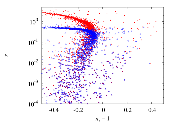
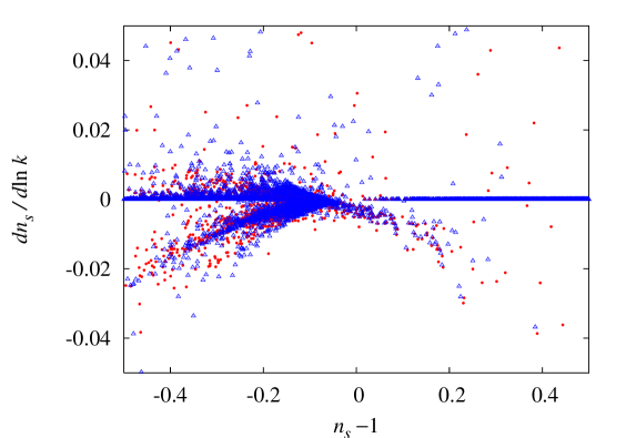
Figure 6: Inflation models generated by the flow equation in the $n_{s}-1$ vs. $r$ plane. Models in the standard scenario are shown in red (circles) while the curvaton cases with $\tilde{f}=5$ are shown in blue (triangles).

Figure 7: Inflation models generated by the flow equation in the $n_{s}-1$ vs. $d\ln n_{s}/dk$ plane. Models in the standard and curvaton scenarios are shown in red (circles) and blue (triangles) respectively.

It is notable that the clustering structure shows up because of relatively large value of $N_{e}$. If a second inflation occurs with the energy density of the curvaton, however, this result may be changed. With the second inflation, significant expansion after the first inflation is possible and hence $N_{e}$ may drastically decrease. When the initial amplitude of the curvaton becomes as large as $M_{\rm pl}$, this can be the case. Then, $N_{e}$ much smaller than $40-70$ may be realized. For some inflation models, reduced value of $N_{e}$ is too small to make the point $(n_{s}-1,r)$ into the clustering region and, consequently, the resulting distribution on the $n_{s}$ vs. $r$ plane becomes more scattered than the previous case. This fact has some importance for models with $-4\epsilon_{H}+2\eta_{H}>1$ (which means that, for some scale, the primordial spectrum is blue-tilted) because the fixed point locates in the region where $n_{s}-1<0$. For models where the initial values of the slow-roll parameters satisfy the relation $-4\epsilon_{H}+2\eta_{H}>1$, the value of $-4\epsilon_{H}+2\eta_{H}$ can be reduced to make $n_{s}-1\simeq 1$ in the course of approaching to the fixed point. As one can see, in the case with the curvaton, larger number of points fall into the region consistent with the WMAP data (i.e., $n_{s}\simeq 1$ with $r\mathop{}_{\textstyle\sim}^{\textstyle<}1$) in Fig. 9 than in Fig. 7.

To be more quantitative, we perform the numerical analysis with smaller values of $N_{e}$. The second inflation driven by the curvaton may decrease the number of $e$-folding $\Delta N_{e}=20-30$. Thus we take the range of the initial $e$-folding number as $10\leq N_{e}\leq 40$ assuming the second inflation due to the curvaton. (In fact, the present horizon scale has to exit the horizon during the first inflation, which gives an upper bound on the initial amplitude of the curvaton. Consequently, in the case with the second inflation, the $\tilde{f}$ parameter cannot be so large; see Eq. (2.23).) The results with the mild value $\tilde{f}=3$ are shown in Figs. 9 and 9 in the $n_{s}$ vs. $r$ and $n_{s}$ vs. $d\ln n_{s}/d\ln k$ planes, respectively. As one can see, compared to the case with $40\leq N_{e}\leq 70$, the distribution is more scattered for $10\leq N_{e}\leq 40$. In particular, sizable number of the inflation models are moved into the region with $n_{s}\simeq 1$, the allowed region from the WMAP data, which is not the case for the case without the second inflation. In fact, in the case with the second inflation, the change of the distribution is mostly from the reduction of the $e$-folding number in the first inflation. Thus, the effects of the curvaton fluctuation (i.e., the values of $\tilde{f}$) on the distribution of models in the $n_{s}$ vs. $r$ plane is not so significant compared with the case with small curvaton initial amplitude.

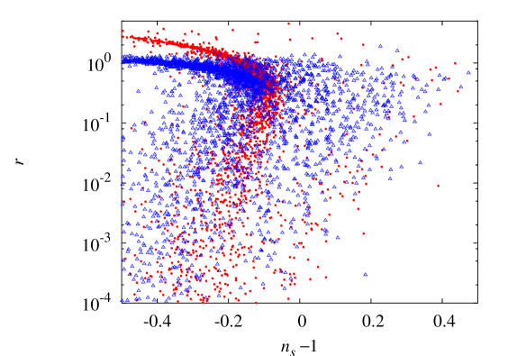
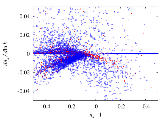
Figure 8: The same as Fig. 7 except that we take $10\leq N_{e}\leq 40$ and $\tilde{f}=3$ for the curvaton case in this figure. (Notice that the data points for the standard case without the curvaton are unchanged.)

Figure 9: The same as Fig. 7 except that we take $10\leq N_{e}\leq 40$ for the curvaton case in this figure.

5 Summary

In this paper, we discussed the effects of the curvaton on inflation models from some general points of view. For this purpose, first we classify inflation models in the $n_{s}$ vs. $r$ plane into three categories: the “small-field” models, “large-field” models and “hybrid-type” models.

For the case that the initial amplitude of the curvaton is small ($\phi_{\rm init}<M_{\rm pl}$) and that the change of $N_{e}$ being negligible, we have shown how the scalar spectral index and the tensor-to-scalar ratio are modified for each models. In the “small-field” models, both the spectral index and the tensor-to-scalar ratio are not affected by the curvaton much (although slight increase in $n_{s}$ can be seen). In the “large-field” models, the spectral index $n_{s}$ always increases and the tensor-to-scalar ratio is largely suppressed. In the “hybrid-type” models, the spectral index always decreases which is the opposite effect compared to the cases with the small-field and large-field models.

We also investigated the effects of the curvaton on inflation models generated by the inflationary flow equation. Since we gave a general argument how the observable quantities are affected by the curvaton, we can easily understand the modification of the structure of distribution of inflation models generated by the inflationary flow equation.

Acknowledgments: T.T. would like to thank the Japan Society for Promotion of Science for financial support. The work of T.M. is supported by the Grants-in Aid of the Ministry of Education, Science, Sports, and Culture of Japan No. 15540247.

References

- [1] C. L. Bennett et al., Astrophys. J. Suppl. 148, 1 (2003) [arXiv:astro-ph/0302207].
- [2] M. Tegmark et al. [SDSS Collaboration], Astrophys. J. 606, 702 (2004) [arXiv:astro-ph/0310725].
- [3] A. H. Guth, Phys. Rev. D 23, 347 (1981); K. Sato, Mon. Not. Roy. Astron. Soc. 195, 467 (1981).
- [4] K. Enqvist and M. S. Sloth, Nucl. Phys. B 626, 395 (2002) [arXiv:hep-ph/0109214]; D. H. Lyth and D. Wands, Phys. Lett. B 524, 5 (2002) [arXiv:hep-ph/0110002]; T. Moroi and T. Takahashi, Phys. Lett. B 522, 215 (2001) [Erratum-ibid. B 539, 303 (2002)] [arXiv:hep-ph/0110096].
- [5] G. Dvali, A. Gruzinov and M. Zaldarriaga, Phys. Rev. D 69, 023505 (2004) [arXiv:astro-ph/0303591].
- [6] L. Kofman, arXiv:astro-ph/0303614.
-
[7]
K. Dimopoulos, D. H. Lyth, A. Notari and A. Riotto,
JHEP 0307, 053 (2003)
[arXiv:hep-ph/0304050];
T. Moroi and H. Murayama, Phys. Lett. B 553, 126 (2003) [arXiv:hep-ph/0211019];
J. McDonald, Phys. Rev. D 68, 043505 (2003) [arXiv:hep-ph/0302222];
M. Postma and A. Mazumdar, JCAP 0401, 005 (2004) [arXiv:hep-ph/0304246];
K. Dimopoulos, G. Lazarides, D. Lyth and R. Ruiz de Austri, JHEP 0305, 057 (2003) [arXiv:hep-ph/0303154];
K. Enqvist, A. Jokinen, S. Kasuya and A. Mazumdar, Phys. Rev. D 68, 103507 (2003) [arXiv:hep-ph/0303165]. - [8] K. Dimopoulos and D. H. Lyth, Phys. Rev. D 69, 123509 (2004) [arXiv:hep-ph/0209180].
- [9] D. H. Lyth, Phys. Lett. B 579, 239 (2004) [arXiv:hep-th/0308110].
- [10] T. Matsuda, Class. Quant. Grav. 21, L11 (2004) [arXiv:hep-ph/0312058].
- [11] M. Postma, JCAP 0405, 002 (2004) [arXiv:astro-ph/0403213].
- [12] K. Dimopoulos, D. H. Lyth and Y. Rodriguez, JHEP 0502, 055 (2005) [arXiv:hep-ph/0411119].
- [13] D. Langlois and F. Vernizzi, Phys. Rev. D 70, 063522 (2004) [arXiv:astro-ph/0403258].
- [14] T. Moroi, T. Takahashi and Y. Toyoda, arXiv:hep-ph/0501007.
- [15] M. B. Hoffman and M. S. Turner, Phys. Rev. D 64, 023506 (2001) [arXiv:astro-ph/0006321].
- [16] W. H. Kinney, Phys. Rev. D 66, 083508 (2002) [arXiv:astro-ph/0206032].
- [17] S. H. Hansen and M. Kunz, Mon. Not. Roy. Astron. Soc. 336, 1007 (2002) [arXiv:hep-ph/0109252].
- [18] R. Easther and W. H. Kinney, Phys. Rev. D 67, 043511 (2003) [arXiv:astro-ph/0210345].
- [19] H. V. Peiris et al., Astrophys. J. Suppl. 148, 213 (2003) [arXiv:astro-ph/0302225].
- [20] W. H. Kinney, E. W. Kolb, A. Melchiorri and A. Riotto, Phys. Rev. D 69, 103516 (2004) [arXiv:hep-ph/0305130].
- [21] A. R. Liddle, Phys. Rev. D 68, 103504 (2003) [arXiv:astro-ph/0307286].
- [22] C. Y. Chen, B. Feng, X. L. Wang and Z. Y. Yang, Class. Quant. Grav. 21, 3223 (2004) [arXiv:astro-ph/0404419].
- [23] E. Ramirez and A. R. Liddle, arXiv:astro-ph/0502361.
- [24] E. D. Stewart and D. H. Lyth, Phys. Lett. B 302, 171 (1993) [arXiv:gr-qc/9302019].
- [25] S. Dodelson, W. H. Kinney and E. W. Kolb, Phys. Rev. D 56, 3207 (1997) [arXiv:astro-ph/9702166].
- [26] T. Moroi and T. Takahashi, Phys. Rev. D 66, 063501 (2002) [arXiv:hep-ph/0206026].
- [27] A. R. Liddle and D. H. Lyth, Cosmological Inflation and Large-Scale Structure (Cambridge University Press, 2000).
- [28] A. R. Liddle and S. M. Leach, Phys. Rev. D 68, 103503 (2003) [arXiv:astro-ph/0305263].