Scalar field models: from the Pioneer anomaly to astrophysical constraints

Abstract

In this work we study how scalar fields may affect solar observables, and use the constraint on the Sun’s central temperature to extract bounds on the parameters of relevant models. Also, a scalar field driven by a suitable potential is shown to produce an anomalous acceleration similar to the one found in the Pioneer anomaly.

1 Introduction

Scalar fields play a fundamental role in contemporary physics, with applications ranging from particle physics to cosmology and condensed matter. In cosmology, these include inflation[1], vacuum energy evolving and quintessence models, the Chaplygin gas dark energy-dark matter unification model and dark matter candidates (for a complete list, see $[2]$ and references within). A scalar field has recently been suggested as a possible explanation for the anomalous acceleration measured by the Pioneer spacecraft[3]. On an astrophysical context, a scalar field could be present as, for example, a mediating boson of an hypothetical fifth force. This can be modelled by a Yukawa potential, given by $V_{Y}(r)=Ae^{-mr}/r$, where $A$ is the coupling strength and $m$ is the mass of the field, setting the range of the interaction $\lambda_{Y}\equiv m^{-1}$. The bounds on parameters $A$ and $\lambda_{Y}\equiv m^{-1}$ can be found in Ref.[4] and references therein. In this work, a scalar field with an appropriate potential is shown to account for the anomalous Pioneer acceleration. Also, the effects of this and other scalar field models on stellar equilibrium is reported.

2 Scalar field induced Pioneer anomaly

The hypothesis that the Pioneer anomaly is due to new physics has been steadily gaining momentum. Fundamentally, this arises because is seems unfeasible that an engineering explanation, affecting spacecrafts with different trajectories and designs, could lead to similar effects. The lack of a simple explanation could hint that this anomalous acceleration is the manifestation of a new force.

Given the broad range of applicability of theories with scalar fields, it is possible that such an entity is responsible for the anomaly[3]. A natural candidate would be the radion, a scalar field present due to oscillations of inter-brane distance in braneworld models. However, this does not account for the phenomena[3]. Fortunately, one can put down a model with a scalar field that doesn’t stray away much from the already accepted theories arising from cosmology. Specifically, we assume a scalar field with dynamics ruled by a potential of the form $V(\phi)=-A^{2}\phi^{-2}$, where $A$ is a constant. The scalar field obeys the equation of motion

$$\phi^{\prime\prime}(r)+{2\over r}\phi^{\prime}(r)=2A^{2}\phi^{-3}~{}~{},$$ (1)

and admits the solution

$$\phi(r)=\left({8\over 3}\right)^{1\over 4}\sqrt{Ar}\equiv\beta^{-1}r^{1\over 2}~{}~{}.$$ (2)

The $0-0$ linearized Einstein’s equations reads

$$f^{\prime\prime}(r)+{2\over r}f^{\prime}(r)=2\kappa\left(1-{2C\over r}\right)A^{2}\beta^{2}r^{-1}$$ (3)

whose solution is

$$f(r)=\sqrt{3\over 2}{A\kappa r\over 2}-\sqrt{6}AC\kappa~{}log\left({r\over 1~{}m}\right)~{}~{}.$$ (4)

The resulting acceleration felt by a test body is given by

$$a_{r}=-{C\over r^{2}}-\sqrt{3\over 2}{A\kappa\over 4}+\sqrt{3\over 2}{AC\kappa\over r}~{}~{}.$$ (5)

The first term is the Newtonian contribution, and identifying the second with the anomalous acceleration $a_{A}=8.5\times 10^{-10}~{}ms^{-2}$, sets $A=3.26~{}a_{A}/\kappa=4.7\times 10^{42}~{}m^{-3}$. The last term is much smaller than the anomalous acceleration for $4C/r\ll 1$, that is, for $r\gg 6~{}km$; it is also much smaller than the Newtonian acceleration for $r\ll~{}2.9\times 10^{22}~{}km\approx 100~{}Mpc$. It has been shown[3] that the effect of this model on the Doppler effect used to calculate the acceleration of the spacecrafts is negligible, indicating that the anomaly is real, an not due to a misinterpreted light propagation.

3 Variable Mass Particle models

The variable mass particle (VAMP) proposal[5] assumes the presence of yet unknown fermions coupled to a dark-energy scalar field with dynamics ruled by a monotonically decreasing potential. Although this has no minima, the coupling of the scalar field $\phi$ to this exotic fermionic matter yields an effective potential of the form $V_{eff}(\phi)=V(\phi)+\lambda n_{\psi}\phi$, where $n_{\phi}$ is the number density of fermionic VAMPs and $\lambda$ is a Yukawa coupling. In the present work we approach a potential of the quintessence-type form, $V(\phi)=u_{0}\phi^{-p}$. As a result, the effective potential acquires a minimum and the related vacuum expectation value (vev) is responsible for the mass term of the exotic VAMP. Since the number density $n_{\psi}$ depends on the scale factor $a(t)$, this mass varies on a cosmological timescale. A noticeable shortcoming of VAMP models is the presence of weakly or unconstrained parameters: the relative density $\Omega_{\psi 0}$, the scalar field coupling constant and the potential strength.

One can attempt to overcome this drawback by assuming that all fermions couple to the quintessence scalar field. This coupling should not substitute the usual Higgs coupling, but merely add a small correction to the Higgs-mechanism induced mass. Since the effects of the quintessence scalar field coupling crucially depend on the particle number density $n_{\psi}$, one expects this variable mass term to play a more relevant role in a stellar environment than in the vacuum. This hints that VAMP model parameters could be constrained from stellar physics observables.

3.1 The polytropic gas stellar model

The polytropic gas model assumes an equation of state of the form $P=K\rho^{n+1/n}$, where $n$ is the polytropic index, defining intermediate processes between the isothermic and adiabatic thermodynamical cases, and $K$ is the polytropic constant, which depends on the star’s mass $M$ and radius $R$. This model leads to scaling laws for thermodynamical quantities, given by $\rho=\rho_{c}\theta^{n}(\xi)$, $T=T_{c}\theta(\xi)$ and $P=P_{c}\theta(\xi)^{n+1}$, where $\rho_{c}$, $T_{c}$ and $P_{c}$ is the density, temperature and pressure at the center of the star[6]. The dimensionless function $\theta(\xi)$ depends on the dimensionless variable $\xi$, related to the distance to the star’s center by $r=\alpha\xi$, where $\alpha$ also depends on the star’s mass $M$ and radius $R$. The hydrostatic equilibrium condition enables a differential equation ruling the behavior of the scaling function $\theta(\xi)$, the Lane-Emden equation:

$${1\over\xi^{2}}{\partial\over\partial\xi}\left(\xi^{2}{\partial\theta\over\partial\xi}\right)=-\theta^{n}~{}~{}.$$ (6)

Since the physical characteristics of a star appear only in the definitions of the constants $K$ and $\alpha$, its stability is independent of these quantities, and different polytropic indexes $n$ label different types of stars. This scale-independence can be related to the homology symmetry enclosed in the Lane-Emden equation. The boundary conditions of this differential equation are, from the definition $\rho=\rho_{c}\theta(\xi)$, $\theta(0)=1$; also, the hydrostatic equilibrium condition implies that $\left|{d\theta/d\xi}\right|_{\xi=0}=0$. The first solar model ever considered corresponds to a polytropic star with $n=3$ and was studied by Eddington in 1926. Although somewhat incomplete, this simplified model gives rise to relevant constraints on the physical quantities.

The following results are based on the luminosity constraint on the Sun’s central temperature, $\Delta T_{c}/T_{c}\leq 0.4\%$. The central temperature can be computed from $T_{c}=Y_{n}\mu GM/R$, where $k$ is the Boltzmann constant and $Y_{n}$ depends on the star’s mass $M$ and radius $R$, as well as on the dimensionless quantity $\xi_{1}$, which is defined through $\theta(\xi_{1})=0$ and signals the surface of the star.

3.2 Results

Assuming isotropy, a variable mass term leads to both a radial, anomalous acceleration $a_{A}=\phi^{\prime}/\phi<0$ plus a time-dependent drag force $a_{D}=-\dot{\phi}/\phi<0$[2]. The time-dependent component should vary on cosmological timescales, and can thus can be absorbed in the usual Higgs mass term. Hence, one considers only the perturbation to the Lane-Emden equation given by the radial force. We start by defining the dimensionless scalar field $\Phi\equiv\phi/\phi_{c}^{*}$, with $\phi_{c}^{*}=\rho_{crit}/2n_{V}$, where $\Omega_{V}$ is the energy density due to the potential driving $\phi$ and $\rho_{crit}\simeq 9.48\times 10^{-28}~{}g~{}cm^{-3}$ is the critical density. Assuming for simplicity a potential with $p=1$, we obtain a perturbed Lane-Emden equation

$${1\over\xi^{2}}{d\over d\xi}\left[\xi^{2}{d\theta\over d\xi}\right]=-\theta^{n}(\xi)-{C_{n}\over U}{1\over\Phi(\xi)}\left[\Phi^{\prime\prime}(\xi)+{2\over\xi}\Phi^{\prime}(\xi)-{\Phi^{\prime 2}(\xi)\over\Phi(\xi)}\right]~{}~{}.$$ (7)

where one has defined the dimensionless quantities

$$U\equiv{GM\over Rc^{2}}=2.12\times 10^{-6}~{}~{},~{}~{}C_{n}^{-1}\equiv(n+1)N_{n}^{n/(n+1)}W_{n}^{1/(n+1)}~{}~{},$$ (8)

with $W_{n}=[4\pi(n+1)\left({d\theta\over d\xi}\right)^{2}_{\xi_{1}}]^{-1}$.

Furthermore, one assumes that the scalar field is only weakly perturbed in relation to the cosmological vev of the effective potential. Denoting this small “astrophysical” contribution as $\Phi_{a}(\xi)$, one has $\Phi(\xi)=\Omega_{V}/\lambda+\Phi_{a}(\xi)$. Hence, the Klein-Gordon equation becomes

$$\Phi^{\prime\prime}_{a}(\xi)+{2\over\xi}\Phi^{\prime}_{a}(\xi)\approx{2\alpha^{2}\lambda n_{V}\over\rho_{crit}}{\rho_{c}\over\mu}\theta^{3}(\xi)-{{2\alpha^{2}\lambda^{2}n_{V}^{2}\over\rho_{crit}}}\left[1-{2\lambda\Phi_{a}(\xi)\over\Omega_{V}}\right]~{}~{},$$ (9)

inside the star, and

$$\Phi^{\prime\prime}_{a}(\xi)+{2\over\xi}\Phi^{\prime}_{a}(\xi)\approx{2\alpha^{2}\lambda n_{V}^{2}\over\rho_{crit}}-{{2\alpha^{2}\lambda^{2}n_{V}^{2}\over\rho_{crit}}}\left[1-{2\lambda\Phi_{a}(\xi)\over\Omega_{V}}\right]~{}~{},$$ (10)

in the outer region. In the above, $n_{\psi}\equiv n_{V}=3~{}m^{-3}$ is the number density of fermions in the vacuum. $\mu$ is the mean molecular weight of Hydrogen. The boundary conditions for the perturbed Lane-Emden are the same as in the unperturbed case. For the scalar field, we assume both $\Phi(\xi)$ and its derivative vanish beyond the Solar System (about $10^{5}~{}AU$). Following[2], one gets that the maximum deviation $\Delta T_{c}/T_{c}=2.82\times 10^{-8}$ occurs for $\Omega_{V}=0.7$, $\lambda=2.82\times 10^{-14}$. Hence, the luminosity constraint is always respected as long as one assumes the bound arising from the assumption that the “astrophysical” component of the scalar field is much smaller than its cosmological vev, $\lambda<10^{-14}$.

4 Yukawa potential induced perturbation

One now looks at the hydrostatic equilibrium equation with a Yukawa potential which, after a small algebraic manipulation, implies the perturbed Lane-Emden equation

$${1\over\xi^{2}}{d\over d\xi}{d\theta\over d\xi}=-\theta^{n}\left[1+Ae^{-\gamma\xi/\xi_{1}}\right]-\gamma AC_{n}{d\theta\over d\xi}e^{-\gamma\xi/\xi_{1}}~{}~{},$$ (11)

where we have defined the dimensionless quantities

$$C_{n}\equiv\left({n+1\over 4\pi}\right)^{1/2}N_{n}^{n/(n+1)}W_{n}^{(1-n)/2(n+1)}~{}~{},~{}~{}\gamma\equiv mR$$ (12)

and $\xi_{1}$ signals the surface of the star (more accurately, a surface of zero temperature, but the difference is negligible. It can be shown that the boundary conditions are unaffected by the perturbation[2].

One can study the variation of the central temperature as a function of $\lambda\equiv m^{-1}$ and $A$, and constraint these so that $\Delta T_{c}/T_{c}\leq 0.4\%$. The parameters were chosen for Yukawa interactions in the range $0.1R<\lambda_{Y}<10R$; the Yukawa coupling $A$ was chosen so that the variation of $T_{c}$ is of the same order $O(10^{-4})$) as the luminosity constraint. Numerical integration of Eq. 11 is then used to derive the exclusion plot of Figure 1, superimposed on the accepted bound[4]. Notice that the central temperature is not precisely known and it is clear that constraining its uncertainty below $10^{-4}$ would yield a larger exclusion region in the parameter space.

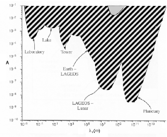
Figure 1: Exclusion plot for the relative deviation from unperturbed central temperature $T_{c}$, for $A$ ranging from $10^{-3}$ to $10^{-1}$, and $\gamma$ from $10^{-1}$ to $10$ (tip at the top), superimposed on the available bounds.

4.1 The Pioneer anomaly

Following a similar procedure to the one depicted in the above two sections, one can prove that a constant, anomalous acceleration $a_{A}$ inside the Sun yields a relative deviation of the central temperature which scales linearly with $a_{A}$ as $\delta T_{c}\sim a_{A}/a_{\odot}$, where $a_{\odot}=274~{}m.s^{-2}$[2]. Thus, the bound $\delta T_{c}<4\times 10^{-3}$ is satisfied for values of this constant anomalous acceleration up to $a_{Max}\sim 10^{-4}a_{\odot}$. The reported value is then well within the allowed region, and has a negligible impact on the astrophysics of the Sun.

5 Conclusion

In this work we have developed a study of the impact of some exotic physics models on stellar equilibrium, enabling the extraction of constraints on the relevant parameters of the theories. Also, a model exhibiting a scalar field with a attractive quintessence-like potential is discussed, which can account for the anomalous acceleration felt by the Pioneer 10/11, Ulysses and Galileo spacecrafts.

References

- [1] See e.g. A. Linde, hep-th/0402051 and K.A. Olive, Phys. Rev. 190 (1990) 307.
- [2] O. Bertolami, J. Páramos Phys. Rev. 71, (2005) 23521.
- [3] O. Bertolami, J. Páramos, Class. Quantum Gravity 21 (2004) 3309.
- [4] “The search for non-Newtonian gravity”, E. Fischbach, C.L. Talmadge (Springer, New York 1999).
- [5] G.W. Anderson, S.M. Carroll, astro-ph/9711288.
- [6] “Textbook of Astronomy and Astrophysics with Elements of Cosmology”, V.B. Bhatia (Narosa Publishing House, Delhi 2001).
- [7] “Theoretical Astrophysics: Stars and Stellar Systems”, T. Padmanabhan (Cambridge University Press, Cambridge 2001).
- [8] J.N. Bahcall, Phys. Rev. D33 (2000) 47.
- [9] J.D. Anderson, P.A. Laing, E.L. Lau, A.S. Liu, M.M. Nieto and S.G. Turyshev, Phys. Rev. D65 (2002) 082004, Phys. Rev. Lett. 81 (1998) 2858.