How to identify the youngest protostars

We study the transition from a prestellar core to a Class 0 protostar, using SPH to simulate the dynamical evolution, and a Monte Carlo radiative transfer code to generate the SED and isophotal maps. For a prestellar core illuminated by the standard interstellar radiation field, the luminosity is low and the SED peaks at $\sim\!190\,\mu{\rm m}$. Once a protostar has formed, the luminosity rises (due to a growing contribution from accretion onto the protostar) and the peak of the SED shifts to shorter wavelengths ($80\;{\rm to}\,100\,\mu{\rm m}$). However, by the end of the Class 0 phase, the accretion rate is falling, the luminosity has decreased, and the peak of the SED shifts back towards longer wavelengths ($90\;{\rm to}\,150\,\mu{\rm m}$). In our simulations, the density of material around the protostar remains sufficiently high well into the Class 0 phase that the protostar only becomes visible in the NIR if it is displaced from the centre dynamically. Raw submm/mm maps of Class 0 protostars tend to be much more centrally condensed than those of prestellar cores. However, when convolved with a typical telescope beam, the difference in central concentration is less marked, although the Class 0 protostars appear more circular. Our results suggest that, if a core is deemed to be prestellar on the basis of having no associated IRAS source, no cm radio emission, and no outflow, but it has a circular appearance and an SED which peaks at wavelengths below $\sim 170\,\mu{\rm m}$, it may well contain a very young Class 0 protostar.

1 Introduction

The details of how molecular clouds form, why they collapse, and how the collapse proceeds to form stars are not very well understood. Over the last two decades, observations of the different stages of this process have lead to an evolutionary scenario of star formation: starless core $\rightarrow$ prestellar core $\rightarrow$ class 0 object $\rightarrow$ class I object $\rightarrow$ class II object $\rightarrow$ class III object (see André et al. 2000).

Starless cores (e.g. Myers et al. 1983; Myers & Benson 1983) are dense cores in molecular clouds in which there is no evidence that star formation has occurred (i.e. no IRAS detection, Beichman et al. 1986). Some of these starless cores are thought to be close to collapse or already collapsing, and they are labelled prestellar cores (Ward-Thompson et al. 1994, 1999); for the rest, it is not always clear whether they are in hydrostatic equilibrium (e.g. Alves et al. 2001 or transient structures within a turbulent cloud (e.g. Ballesteros-Paredes et al. 2003). Prestellar cores have been observed both in relative isolation (e.g. L1544, L63; Ward-Thompson et al. 1999) and in protoclusters (e.g. $\rho$ Oph, Motte et al. 1998; NGC 2068/2071, Motte et al. 2001). They have typical sizes $(1-20)\times 10^{3}$ AU and masses from $0.05$ to $35\,{\rm M}_{\sun}$. From statistical arguments (e.g. André et al. 2000) it is inferred that prestellar cores live only a few million years.

Class 0 objects represent the stage when a protostar has just been formed in the centre of the core, but the protostar is still less massive than its surrounding envelope (André et al. 1993). The protostar is deeply embedded in the core and cannot be observed directly, but its presence can often be inferred from bipolar molecular outflows or compact centimetre radio emission. The Class 0 phase last for a few $10^{4}\,{\rm years}$ and is characterised by a large accretion rate ($\ga 10^{-5}\,{\rm M}_{\sun}$/yr). Most of the mass of the protostar is delivered during this phase (e.g. Whitworth & Ward-Thompson 2001).

Once the protostar becomes more massive than its surrounding envelope, the core enters the Class I phase. Accretion onto the central protostar, or onto the disc around the protostar, continues, but at a lower rate ($\la 10^{-6}\,{\rm M}_{\sun}$/yr). This phase lasts for a few $10^{5}\,{\rm years}$, and delivers most of the rest of the mass of the protostar.

Finally, Class II and Class III objects correspond to even later stages of star formation, when most of the envelope has disappeared, and the star is visible in the optical. Class I objects are classical T Tauri stars (CTTSs), with ongoing accretion (but at much lower levels than before, $\la 10^{-8}\,{\rm M}_{\sun}$/yr) and well defined discs. Class III objects are weak-line T Tauri stars (WTTs) with little sign of accretion and no inner disc.

In their quest to identify the youngest protostars, André et al. (1993, 2000) set 3 criteria for classifying an object as Class 0: (i) the presence of a central luminosity source, as indicated by the detection of a compact centimetre radio source, or a bipolar molecular outflow, or internal heating; (ii) centrally peaked but extended submillimetre continuum emission, indicating the presence of an envelope around the central source; and (iii) a high ratio ($>0.005$) of submillimetre to bolometric luminosity, where the submillimetre is defined as $\lambda\ga 350\,\mu{\rm m}$. Criteria (ii) and (iii) are used to distinguish between Class 0 and Class I objects, whereas criterion (i) is used to distinguish between Class 0 objects and prestellar cores. However, criterion (i) may be inadequate to distinguish between the youngest Class 0 objects and the oldest prestellar cores: (a) the cm emission may be be too weak to be observed, especially in the earliest stages of protostar formation; (b) the region may be too complex for the molecular outflows to be detectable; and (c) internal heating may be difficult to establish, if the protostar is deeply embedded in the core.

The origin of radio emission from Class 0 objects is uncertain (cf. Gibb 1999). Theoretical models show that once a protostar forms at the centre of a collapsing core, the infalling gas accelerates to supersonic velocities and an accretion shock develops on the surface of the protostar and/or on the surface of the disc that surrounds the protostar (Winkler & Newman 1980, Cassen & Moosman 1981). The heating provided by the shock ionises the surrounding gas, which then emits free-free radio radiation (e.g. Bertout 1983; Neufeld & Hollenbach 1994, 1996). The radio luminosity depends on the mass of the protostar, the accretion rate and the observer’s viewing angle. For a low-mass protostar, $\la{\rm M}_{\sun}$, the predicted flux is below detection limits (Neufeld & Hollenbach 1996), unless the accretion rate is high, $\ga 10^{-5}\,{\rm M}_{\sun}$/yr. Another possibility is that the radio emission is produced by an ionised disc wind (e.g. Martin 1996), or from a partially ionised jet that emanates from the protostar and propagates into the collapsing envelope producing shocks (Curiel et al. 1987). The detection of radio emission from many Class 0 protostars, using the VLA (e.g. Bontemps et al. 1995), points toward the latter two explanations.

Recently Young et al. (2004), using the Spitzer space telescope, detected NIR radiation from L1014, a dense core that was previously classified as prestellar. The detection of NIR radiation strongly suggests that this is a young Class 0 object, and supports the view that even younger Class 0 objects may not be detectable in the NIR, with IRAS, or even with Spitzer.

The goal of this paper is to study the transition from prestellar cores to Class 0 objects, and to seek new criteria for distinguishing between these two stages, in particular criteria which can be used before the standard signatures of protostar birth, such as compact radio emission and/or bipolar molecular outflows, become detectable. We use SPH to simulate to the dynamics of a collapsing molecular core, and a Monte Carlo code to treat the transfer of radiation within the core. The radiative transfer is treated fully in 3D, which is important for the correct interpretation of the observations (cf. Boss & Yorke 1990; Whitney et al. 2003a, 2003b; Steinacker et al. 2004). We use a newly developed method for performing Monte Carlo radiative transfer simulations on SPH density fields, which constructs radiative transfer cells using the SPH tree structure (Stamatellos 2003; Stamatellos & Whitworth 2005, hereafter Paper I).

In Section 2 we describe the SPH simulation of the collapse of a turbulent molecular core. In Section 3 we describe the radiative transfer method, focusing on how we construct radiative transfer cells. We also discuss the radiation sources and the properties of the dust used in our model. In Section 4 we present our results for the dust temperature fields, SEDs and isophotal maps of prestellar cores and young Class 0 protostars. In Section 5 we discuss how SEDs and isophotal maps at submm and mm wavelengths might be used to distinguish between late-phase prestellar cores and early-phase Class 0 objects. In Section 6 we summarise our results.

2 The SPH simulation

We use the Smoothed Particle Hydrodynamics code dragon (Goodwin et al. 2004a) to simulate the collapse of a turbulent molecular core and the resulting star formation. Here, we briefly describe the main elements of the model. For a more detailed discussion we refer to Goodwin et al. (2004b).

The initial conditions in the core, before the start of collapse, are dictated by observations of prestellar cores (e.g. Ward-Thompson et al. 1999, Alves et al. 2001). Prestellar cores appear to have approximately uniform density in their central regions, and the density then falls off in the envelope. If the density in the envelope is fitted with a power law, $n(r)\propto r^{-\eta}\,$, then $\eta\sim 2\,{\rm to}\,4\,$. Here $\eta\sim 2$ is characteristic of more extended prestellar cores in dispersed star formation regions (e.g. L1544, L63 and L43), whereas $\eta\sim 4$ is characteristic of more compact cores in protoclusters (e.g. $\rho$ Oph and NGC2068/2071). These features can be represented by a Plummer-like density profile (Plummer 1915),

$$\rho=\frac{\rho_{{}_{0}}}{\left(1+(r/r_{{}_{0}})^{2}\right)^{2}}\,,\;\;\;\;r<r_{{}_{\rm B}}$$ (1)

The density profile is almost flat for $r<r_{{}_{0}}$, and falls off as $r^{-4}$ in the outer envelope ($r>r_{{}_{0}}$). We set $\rho_{{}_{0}}=3\times 10^{-18}\,{\rm g\,cm}^{-3}$, $r_{{}_{0}}=5,000\,{\rm AU}$, and $r_{{}_{\rm B}}=50,000\,{\rm AU}$. The core mass is then 5.4 M_☉. The core is initially isothermal at 10 K, hence the thermal virial ratio is $\alpha_{{}_{\rm THERM}}\equiv E_{{}_{\rm THERM}}/|E_{{}_{\rm GRAV}}|=0.45$. Observations of star forming cores (e.g. Jijina et al. 1999) show that their line widths have a non-thermal contribution, which may be due to turbulence. We impose a low level of turbulence ($\alpha_{{}_{\rm TURB}}\equiv E_{{}_{\rm TURB}}/|E_{{}_{\rm GRAV}}|=0.05$) with a power spectrum $P(k)\propto k^{-4}$ so as to mimic the observed scaling relation between linear size and internal velocity dispersion (Larson 1981).

Collapse of the turbulent core leads to the formation of a single star surrounded by a disc, and the material in the disc then slowly accretes onto the star. A sink particle, representing the star and the inner part of the disc, is created where the density first exceeds $\rho_{{}_{\rm CRIT}}=10^{-11}\,{\rm g\,cm}^{-3}$, and incorporating all the matter within $R_{{}_{\rm INIT}}=5\,{\rm AU}$ of this point (Bate et al. 1995). (The values of $\rho_{{}_{\rm CRIT}}$ and $R_{{}_{\rm INIT}}$ are dictated by computational constraints. If $\rho_{{}_{\rm CRIT}}$ is increased, $R_{{}_{\rm INIT}}$ must be reduced, and more computational time is needed.)

We use a newly developed type of sink called a smartie, which is a rotating oblate spheroid with radius $R_{{}_{\rm S}}$ and half-thickness $Z_{{}_{\rm S}}$ (Fig. 1). The star is a point mass $M_{{}_{\star}}$ at the centre of the smartie, and the spheroid represents the inner part of the accretion disc surrounding the star. $R_{{}_{\rm S}}$ and $Z_{{}_{\rm S}}$ are calculated by assuming that the inner part of the accretion disc (the part inside the spheroid) has uniform density, temperature and angular speed, and that its internal energy and spin angular momentum balance its self-gravity and the gravity of the central star.

The SPH particles which enter the smartie during a timestep, $(t,t+\Delta t)$, are assimilated by it at the end of the timestep, $t+\Delta t$, and their mass is initially added to the mass of the smartie, $M_{{}_{\rm S}}$, i.e. to the mass of the inner disc,

$$M_{{}_{\rm S}}^{\prime}\;=\;{M}_{{}_{\rm S}}\,+\,\sum_{i}\left\{m_{i}\right\}\,.$$ (2)

At the same time, the centre of mass, ${\bf R}_{{}_{\rm S}}$, and velocity, ${\bf V}_{{}_{\rm S}}$, of the smartie are adjusted to conserve linear momentum,

$${\bf R}_{{}_{\rm S}}^{\prime} = \frac{M_{{}_{\rm S}}{\bf R}_{{}_{\rm S}}\,+\,\sum_{i}\left\{m_{i}{\bf r}_{i}\right\}}{M_{{}_{\rm S}}^{\prime}}\,,$$ (3)

$${\bf V}_{{}_{\rm S}}^{\prime} = \frac{M_{{}_{\rm S}}{\bf V}_{{}_{\rm S}}\,+\,\sum_{i}\left\{m_{i}{\bf v}_{i}\right\}}{M_{{}_{\rm S}}^{\prime}}\,,$$ (4)

and the intrinsic angular momentum (spin) of the smartie is adjusted to conserve angular momentum,

$${\bf H}_{{}_{\rm S}}^{\prime} = {\bf H}_{{}_{\rm S}}\,+\,M_{{}_{\rm S}}\left({\bf R}_{{}_{\rm S}}-{\bf R}_{{}_{\rm S}}^{\prime}\right)\otimes\left({\bf V}_{{}_{\rm S}}-{\bf V}_{{}_{\rm S}}^{\prime}\right)$$ (5)

$$\hskip 5.69046pt\,+\,\sum_{i}\left\{m_{i}\left({\bf r}_{i}-{\bf R}_{{}_{\rm S}}^{\prime}\right)\otimes\left({\bf v}_{i}-{\bf V}_{{}_{\rm S}}^{\prime}\right)\right\}\,.$$

In Eqns, 2 through 5, primed variables ($M_{{}_{\rm S}}^{\prime}$, ${\bf R}_{{}_{\rm S}}^{\prime}$, ${\bf V}_{{}_{\rm S}}^{\prime}$, ${\bf H}_{{}_{\rm S}}^{\prime}$) are used to denote sink parameters adjusted for the addition of assimilated SPH particles.

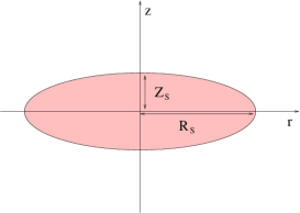
Figure 1: We use an oblate spheroidal sink particle, called a smartie, which contains a central star and a disc, and launches a bipolar outflow.

The smartie mass evolves according to

$$\frac{dM_{{}_{\rm S}}}{dt}\;=\;\left.\frac{dM}{dt}\right|_{{}_{\rm IN}}\,-\,\frac{dM_{{}_{\star}}}{dt}\,-\,\left.\frac{dM}{dt}\right|_{{}_{\rm OUT}}\,,$$ (6)

where the first term on the right of Eqn. 6 represents SPH particles assimilated by the smartie, as discussed in the preceding paragraph.

The second term on the right of Eqn. 6 represents accretion onto the central star, and is given by

$$\frac{dM_{{}_{\star}}}{dt} = -\,\frac{0.9M_{{}_{\rm S}}}{t_{{}_{\rm VISC}}}\,,$$ (7)

$$t_{{}_{\rm VISC}} = \frac{\left[G(M_{{}_{\star}}+M_{{}_{\rm S}})R_{{}_{\rm S}}\right]^{1/2}}{\alpha_{{}_{\rm SS}}\,a_{{}_{\rm S}}^{2}}\,\left\{1\,+\,\frac{GM_{{}_{\rm S}}^{2}}{(M_{{}_{\star}}+M_{{}_{\rm S}})R_{{}_{\rm S}}a_{{}_{\rm S}}^{2}}\right\}^{-1}\,,$$ (8)

where $\alpha_{{}_{\rm SS}}$ is the standard Shakura & Sunyaev (1973) turbulent viscosity parameter and $a_{{}_{\rm S}}$ is the mean sound speed in the smartie. The leading term represents turbulent viscosity, and the term in braces adjusts this for angular momentum transport by gravitational torques in a Toomre-unstable disc (cf. Lin & Pringle 1990).

The third term on the right of Eqn. 6 represents mass loss from the smartie, which can occur in two ways. (i) SPH particles are created at rate $0.1M_{{}_{\rm S}}/t_{{}_{\rm VISC}}$ and launched along the rotation axis with speed $100\,{\rm km\,s}^{-1}$ to form a bipolar outflow. These jets push the surrounding material aside and create hourglass cavities about the rotation axis. (ii) In the present model the outflow does not remove any angular momentum. Therefore the redistribution of angular momentum which drives accretion onto the central star causes the residual inner disc (which has to carry all the angular momentum assimilated by the smartie) to expand. When this happens, the smartie is allowed to expand until $R_{{}_{\rm S}}=16\,{\rm AU}$. Thereafter, $R_{{}_{\rm S}}$ is held constant by excreting SPH particles – and with them angular momentum – just outside the equator of the smartie.

The luminosity of the star is given by

$$L_{{}_{\star}}\;=\;{\rm L}_{{}_{\odot}}\left(\frac{M_{{}_{\star}}}{{\rm M}_{{}_{\odot}}}\right)^{3}\,+\,\frac{GM_{{}_{\star}}}{R_{{}_{\star}}}\frac{dM_{{}_{\star}}}{dt}\,,$$ (9)

where $M_{{}_{\star}}$ and $R_{{}_{\star}}$ are the mass and radius of the star, and we set $R_{{}_{\star}}=3{\rm R}_{{}_{\odot}}$ (Stahler 1988).

The mean smartie temperature, and hence also the mean smartie sound speed, are determined by the balance between radiative cooling, heating by radiation from the star and from the background radiation field, and viscous dissipation in the inspiralling gas of the smartie. A full description of the implementation of smarties is given in Boyd (2003), and the consequences of feedback from bipolar outflows are explored in detail in Boyd et al. (in preparation).

3 The radiative transfer simulation

For the radiative transfer simulations, we use a version of phaethon, a Monte Carlo radiative transfer code which we have developed (Stamatellos & Whitworth 2003) and optimised for radiative transfer simulations on SPH density fields (Paper I). The main developments of the optimised version are (i) that it uses the tree structure inherent within the SPH code to construct a grid of cubic radiative transfer (RT) cells, spanning the entire computational domain, the global grid; and (ii) that in addition it constructs a local grid of concentric spherical RT cells around each star, a star grid, to capture the steep temperature gradients that are expected in the vicinity of a star. The code reemits luminosity packets are soon as they are absorbed (Lucy 1999) and uses the frequency distribution adjustment technique developed by Bjorkman & Wood (2000).

3.1 Construction of the global radiative transfer grid

To construct RT cells for a given time-frame from an SPH simulation, we take advantage of the fact that SPH uses an octal tree structure (to group particles together when calculating gravity forces and also to find neighbours; for details see Paper I). The SPH tree is a recursive hierarchical division of the computational domain into cubic cells within cubic cells (Barnes & Hut 1986). When the SPH tree is being built, we record information about the size of each cell and the number of SPH particles it contains. The RT cells of the global grid are then the largest SPH cells which contain $\leq N_{{}_{\rm MAX}}$ particles. This means that the RT cells automatically have comparable mass. We choose $N_{{}_{\rm MAX}}\sim 100\;{\rm to}\;150$, i.e. somewhat larger than the mean number of SPH neighbours, $N_{{}_{\rm NEIB}}\sim 50$. Consequently the size of the RT cells is on the order of the smoothing length, $h$, and so the temperature resolution is similar to the density resolution of the SPH simulation.

In order to increase the resolution of the radiative transfer simulation, we use particle splitting (Kitsionas & Whitworth 2002). This method replaces each SPH particle (parent particle) with a small group of 13 particles (children particles), each one having 1/13 of the mass of the parent particle. The children are placed on an hexagonal close-packed array, with one of them in the centre of the array and the other 12 equidistant from the first one. By doing this the smoothing length is decreased by a factor of $13^{-1/3}=0.425$, and the average size of the radiative transfer cells is reduced by the same factor.

3.2 Construction of the local radiative transfer grid around a star

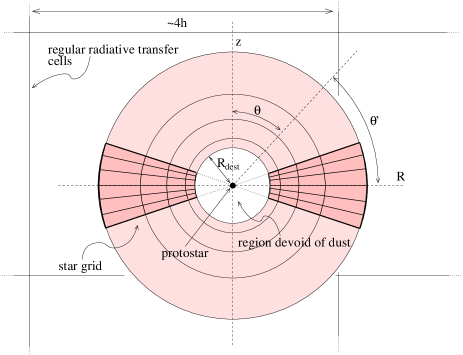
Figure 2: The star grid consists of concentric spherical surfaces centred on the star, with equal spacing in $\log(r)$, and conical surfaces symmetric about the angular momentum of the smartie, with equally spaced opening angle $\theta$. This grid takes account of the dust-free cavity in the immediate vicinity of the star, and resolves the disc inside the smartie.

In Paper I we discussed the need for a high-resolution grid of radiative transfer cells – a star grid – in order to capture the steep temperature gradients that are expected in the vicinity of a star. The star grid discussed there was developed for treating the unresolved region inside a spherically symmetric sink, and so a one-dimensional star grid consisting of concentric spherical cells centred on the star was sufficient.

In the case we examine here the sinks are smarties, i.e. oblate spheroids, and the unresolved region inside a smartie represents both the protostar and the inner protostellar disc. Thus a spherically symmetric one-dimensional star grid is inappropriate. Instead we adopt a similar approach to Kurosawa et al. (2004) and represent the unresolved region near the star with a flared disc (Fig. 2).

However, the properties of the inner disc are not imposed externally, as in Kurosawa et al. (2004), but are determined by the properties of the smartie, and therefore attempt to capture the physics of a protostellar disc accreting onto a newly-formed protostar (as outlined in Section 2). Specifically, we adopt an inner disc with inner radius $R_{{}_{\rm DEST}}$, outer radius $R_{{}_{\rm SG}}$, and constant ratio of thickness, $H$, to radius, $r$,

$$H(r)\;=\;\alpha\,r\,,\;\;\;\;{\rm where}\;\;\;\;\alpha\;=\;\frac{Z_{{}_{\rm S}}}{R_{{}_{\rm S}}}\,.$$ (10)

The dust destruction radius is given by

$$R_{{}_{\rm DEST}}\;=\;\frac{R_{{}_{\star}}}{2}\,\left(\frac{T_{{}_{\star}}}{T_{{}_{\rm DEST}}}\right)^{(4+\beta)/2}\,,$$ (11)

where $\beta$ is the dust emissivity index (see Paper I). There is no dust inside $R_{{}_{\rm DEST}}$.

We put $R_{\rm SG}=16\,{\rm AU}$, since this is the maximum size of a smartie, and it is comparable with the size of the local global RT cells (the cubic cells constructed from the SPH tree).

For $z<4\alpha r$ and $R_{{}_{\rm DEST}}<r<R_{{}_{\rm SG}}$, the density of the inner disc is given by

$$\rho(z,r)=\rho_{{}_{\rm DEST}}\,\left(\frac{r}{R_{{}_{\rm DEST}}}\right)^{-2}\,\exp\left[-\,\frac{1}{2}\left(\frac{z}{\alpha r}\right)^{2}\right]\,,$$ (12)

(cf. Wood et al. 2002a, 2002b). $\rho_{{}_{\rm DEST}}$ is fixed by equating the mass of this inner disc to the mass of the disc inside the smartie. For $z>4\alpha r$ and $R_{{}_{\rm DEST}}<r<R_{{}_{\rm SG}}$, the density is set equal to the average density of the local global RT cells.

The inner disc is then divided into RT cells by spherical and conical surfaces (see Fig. 2). The spherical surfaces are evenly spaced in logarithmic radius and there are typically 20 of them. The conical surfaces are evenly spaced in polar angle and there are typically 30 of them.

3.3 Radiation sources

Figure 3: Dotted line: The external illumination field (BISRF + emission from PAHs). Solid line: The radiation scattered by the molecular cloud. This is similar for all the time-frames and viewing angles, for the models we examine here.

Table 1: Model parameters

id	time (yr)	$M_{\star}({\rm M}_{\sun})$	$R_{\rm S}$ (AU)	$Z_{\rm S}$ (AU)	$M_{\rm S}({\rm M}_{\sun})$	$\dot{M}_{\star}({\rm M}_{\sun}$/yr)	$L_{\rm TOT}({\rm L}_{\sun})$	$T_{\star}$ (K)	description
t0	0	-	-	-	-	-	-	-	initial conditions
t1	$5.3\times 10^{4}$	-	-	-	-	-	-	-	before sink formation
t2	$5.3\times 10^{4}$	0.01	4.0	3.4	0.04	$5\times 10^{-5}$	5.7	5150	a protostar has formed
t3	$6.0\times 10^{4}$	0.20	4.0	0.4	0.09	$1\times 10^{-5}$	27.2	7650
t4	$6.8\times 10^{4}$	0.49	4.0	0.4	0.05	$2\times 10^{-6}$	12.3	6250
t5	$6.9\times 10^{4}$	0.53	4.0	0.4	0.01	$4\times 10^{-7}$	2.5	4200	protostar is off centre

$Z_{\rm S}$, $R_{\rm S}$: Smartie dimensions (Fig. 1)	$M_{\rm\star}$: Stellar mass	$T_{\star}$: Star temperature
$M_{\rm S}$: Smartie mass	$\dot{M}_{\star}$: Accretion rate onto the central star	$L_{\rm TOT}$: Total star luminosity (intrinsic +accretion)

The core is illuminated externally by the interstellar radiation field and internally by the newly formed protostar (once it has formed).

For the external radiation field we adopt a revised version of the Black (1994) interstellar radiation field (BISRF). The BISRF consists of radiation from giant stars and dwarfs, thermal emission from dust grains, cosmic background radiation, and mid-infrared emission from transiently heated small PAH grains (André et al. 2003), as illustrated on Fig. 3. Typically the BISRF is represented by $10^{9}-10^{10}$ $L$-packets (see Paper I).

The protostar luminosity, $L_{{}_{\star}}$, and effective temperature, $T_{{}_{\star}}$ are given by Eqn. 9; a blackbody spectrum at $T_{{}_{\star}}$ is assumed. For the systems examined here, the accretion contribution to the luminosity dominates, because the mass of the protostar is small ($<0.6\,{\rm M}_{\sun}$) and the accretion rate is high ($>10^{-7}\,{\rm M}_{\sun}$/yr). Typically the protostar is represented by $10^{6}\;{\rm to}\;10^{8}$ $L$-packets.

3.4 Dust opacity

Like other studies of prestellar cores (e.g. Evans et al. 2001, Young et al. 2004) we use the Ossenkopf & Henning (1994) opacity for a standard MRN interstellar grain mixture (53% silicate and 47% graphite) which has coagulated and accreted thin ice mantles over a period of $10^{5}$ yr at a density of $10^{6}\;{\rm cm}^{-3}$. However, we emphasize that the opacity of the dust in cores is very uncertain (e.g. Bianchi et al. 2003).

4 The evolution of the dust temperature field, SED and isophotal maps in a star-forming core

We perform radiative transfer simulations on 6 time-frames during the collapse of a star-forming core. We focus our attention just before and just after the formation of the first protostar in the core. The characteristics of each time-frame are listed in Table 1. The simulations are 3-dimensional and provide dust temperature fields, SEDs and isophotal maps.

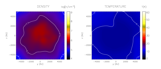
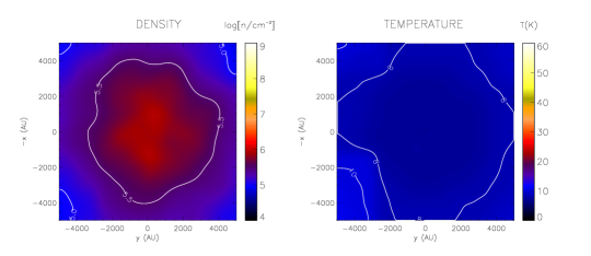
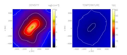
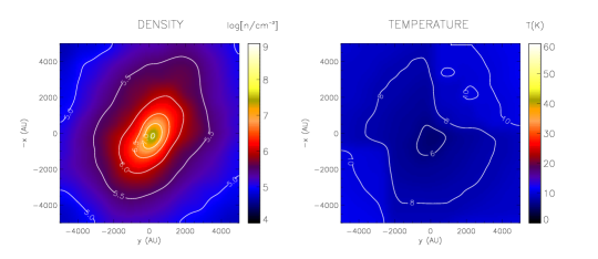
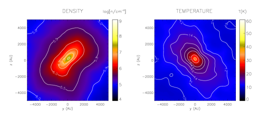
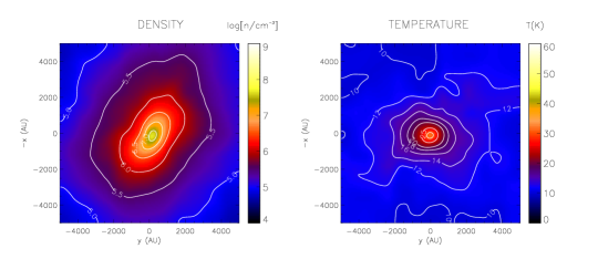
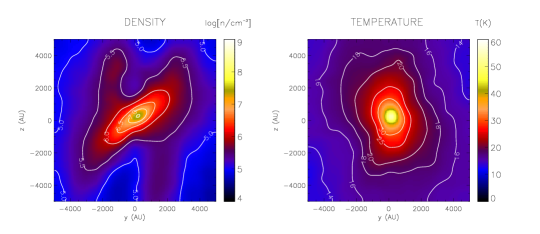
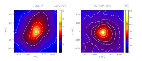
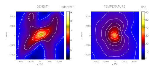
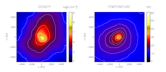
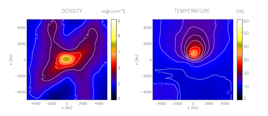
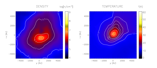
Figure 4: Cross sections of density and dust temperature on a plane parallel to the $x=0$ plane (left two columns) and parallel to the $z=0$ plane (right two columns). Each row corresponds to a different time frame from Table 1, top to bottom t0 to t5. The planes are chosen so as to include the maximum density region (t0 and t1) or the protostar (t2 to t5).

4.1 Dust temperature fields in prestellar cores and young protostars

In Fig. 4 we present the density fields and dust-temperature fields for the 6 time-frames in Table 1. We plot the density and the temperature on 2 cuts through the computational domain, one parallel to the $x=0$ plane and one parallel to the $z=0$ plane. Each of these planes passes through the protostar, or, if there is no protostar (as in the first 2 time-frames), through the densest part of the core. The plots show only the central region of the core ($5000\,{\rm AU}\times 5000\,{\rm AU}$). Additionally, on Fig. 5, we plot the density and the temperature of each RT cell versus distance $r$ from the centre of coordinates, on a logarithmic scale, in order to depict better the regions very close to the protostar.

Our results for the temperature are broadly similar to those of previous 1D and 2D studies of prestellar cores and Class 0 objects. Before the collapse, the precollapse prestellar core is quite cold ($10\;{\rm to}\,20\,{\rm K}$) and it becomes even colder ($5\;{\rm to}\,20\,{\rm K}$) as the collapse proceeds and the central regions become very dense and opaque. As soon as a protostar forms, the region around it becomes very hot (up to the dust destruction temperature), but the temperature still drops below $\sim\!20\,{\rm K}$ beyond a few $1000\,{\rm AU}$ from the protostar, because of the high optical depth in the dense accretion flow onto the protostar. The luminosity of the protostar is dominated by the contribution from accretion. Initially the accretion luminosity increases due to the increasing mass of the protostar, but then it falls as the accretion rate declines.

4.2 SEDs of prestellar cores and young protostars

The SEDs of the 6 time-frames in Table 1 are presented in Fig. 6. These SEDs have been calculated assuming that the core is at $140\,{\rm pc}$. SEDs are plotted for 6 different viewing angles, i.e. 3 polar angles ($\theta=0\degr$, $45\degr$, $90\degr$) and 2 azimuthal angles ($\phi=0\degr$, $90\degr$). Hence on each graph there are 6 curves. However, in several cases the SED is so weakly dependent on viewing angle that the curves overlap. We plot only the thermal emission from the core, i.e. we neglect both the long-wavelength background radiation that just passes through the cloud, and the short-wavelength radiation that is scattered by the outer layers of the cloud.

The effective temperature of the core, as inferred from the peak of the SED, rises and falls with the accretion luminosity of the protostar. For a prestellar core, the SED peaks at $\sim 190\,\mu{\rm m}$, implying $T_{{}_{\rm EFF}}\sim 13\,{\rm K}$. Once the protostar has formed and inputs energy into the system, the peak moves steadily to shorter wavelengths, reaching $\sim 80\,\mu{\rm m}$ ($T_{{}_{\rm EFF}}\sim 31\,{\rm K}$) as the accretion luminosity reaches its maximum, and then moving back to longer wavelengths again as the accretion luminosity declines. By the final frame it has reached $\sim 150\,\mu{\rm m}$ ($T_{{}_{\rm EFF}}\sim 17\,{\rm K}$).

The peak of the SED of a prestellar core is independent of viewing angle, since the core is optically thin to the radiation it emits. In contrast, the peak of the SED of a Class 0 object does depend on viewing angle, albeit weakly, because of the presence of an optically thick disc around the protostar. However, even allowing for variations in the viewing angle, the SED of a Class 0 object does not peak at the wavelengths characteristic of prestellar cores ($\sim 190\,\mu{\rm m}$).

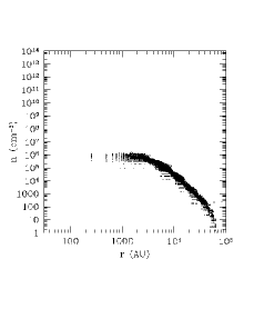
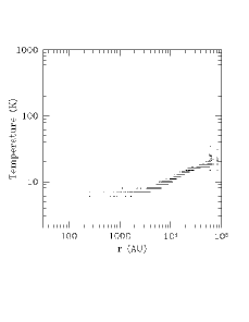
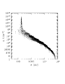
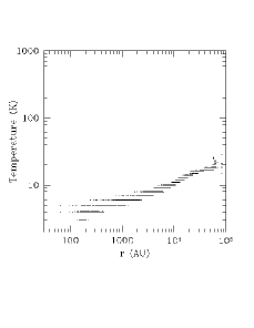
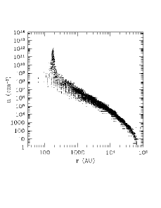
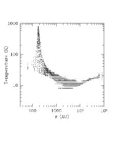
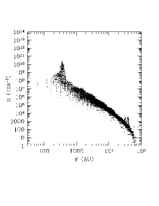
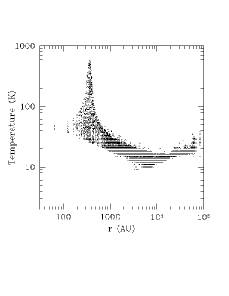
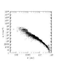
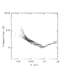
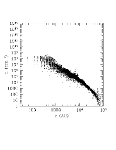
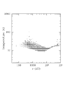
Figure 5: Log-log plot of density (left column) and dust temperature (right column) versus distance from the centre of coordinates, in a collapsing core which forms a protostar; from top to bottom, time-frames t0 to t5 (see Table 1).

4.3 Is a young Class 0 observable in the NIR?

Our model predicts that a young protostar embedded in a core is not observable in the NIR, unless the protostar is displaced from the central high-density region. This contradicts the recent results of Whitney et al. (2003b) and Young et al. (2004). We attribute the difference between our model and that of Young et al. to the density they use for the region around the protostar ($\sim 10^{5}\,{\rm cm}^{-3}$), which may be too low for a Class 0 objects and more appropriate for a prestellar core. Whitney et al. use a higher density in the central region ($\sim 10^{10}\,{\rm cm}^{-3}$), but it is still more than one order of magnitude lower than the density produced by our SPH simulation ($\sim 3\times 10^{12}\,{\rm cm}^{-3}$). Additionally, they use different dust properties for the different regions in their configuration (cloud, disc mid-plane, disc atmosphere, outflow); in particular, the opacity of their dust in the disc midplane is smaller than the opacity in our model, at wavelengths shorter than $10\,\mu{\rm m}$. There are also some differences in the properties of the discs used in the different models, but these are less relevant to the escape of NIR radiation.

The models reported by Shirley et al. (2002) use central densities and dust opacities similar to our models, but they confine their study to the FIR/mm region of the spectrum, so a comparison is not possible.

Ultimately, the density distribution within $500\,{\rm AU}$ of the centre of a core or protostar is not well constrained by observations, and therefore radiative transfer calculations have to rely on theoretical models of core collapse. Dust opacities are also poorly constrained (e.g. Bianchi et al. 2003). Comparison of our model with those of Whitney et al. (2003b) and Young et al. (2004) suggests that the presence or absence of NIR emission from a confirmed Class 0 object might be used to constrain the density profile within a few $100\,{\rm AU}$ of the protostar and/or the opacity of the dust in the same region.

Figure 6: SEDs of the 6 time-frames in Table 1, from 3 polar angles ($\theta=0\degr$, $45\degr$, $90\degr$) and 2 azimuthal angles ($\phi=0\degr$, $90\degr$); in several cases the SEDs from different viewing angles overlap. (a) t0 - precollapse prestellar core. The SED peaks at $\sim 190\,\mu{\rm m}$, which implies an effective temperature $T_{{}_{\rm EFF}}\sim 13\,{\rm K}$. (b) t1 - collapsing prestellar core. The SED appears the same as in (a) although the collapse has started and the cloud is denser and colder at its centre. (c) t2 - Class 0 object. The emission of the system peaks at $\lambda\sim 100\;{\rm to}\,135\,\mu{\rm m}$ (depending on the observer’s viewing angle), which implies $T_{{}_{\rm EFF}}\sim 18\,{\rm to}\,25\,{\rm K}$. The total luminosity of the system is higher than in (b). (d) t3 - Class 0 object. Similar to (c), but the luminosity is even higher, and the SED peaks at $\lambda\sim 80\;{\rm to}\,100\,\mu{\rm m}$, implying $T_{{}_{\rm EFF}}\sim 25\;{\rm to}\,31\,{\rm K}$. (e) t4 - Class 0 object. Similar to (d), but the luminosity has started to decrease due to the falling accretion rate, and the SED peaks at $\lambda\sim 90\;{\rm to}\,135\,\mu{\rm m}$, implying $T_{{}_{\rm EFF}}\sim 18\;{\rm to}\,28\,{\rm K}$. (f) t5 - Class 0 object. The protostar has moved out of the central region by $\sim 100\,{\rm AU}$, and the attenuated stellar emission can be seen at short wavelengths ($1\;{\rm to}\,50\,\mu{\rm m}$). The peak of the cloud emission is at $\lambda\sim 150\,\mu{\rm m}$, implying $T_{{}_{\rm EFF}}\sim 17\,{\rm K}$.

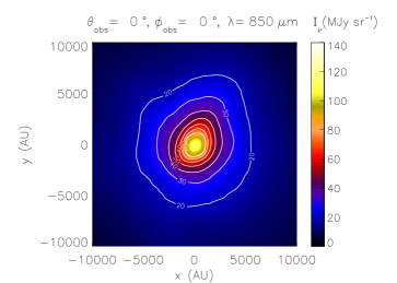
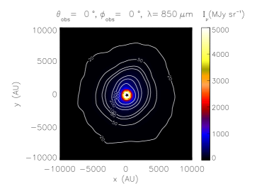
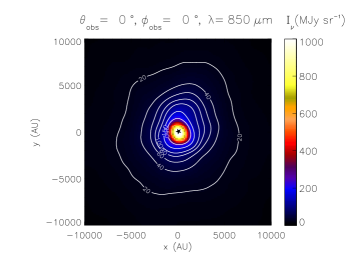
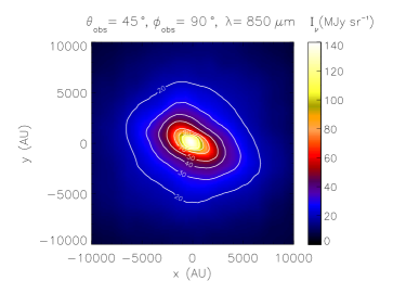
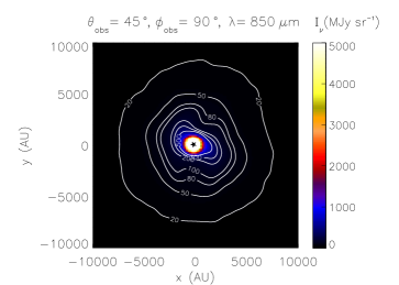
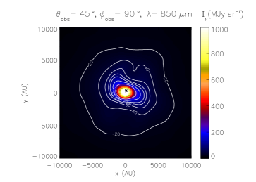
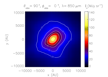
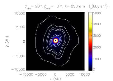
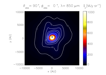
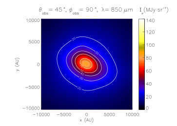
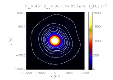
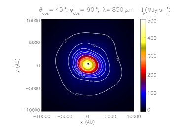
Figure 7: 850 $\mu{\rm m}$ isophotal maps of 3 different time-frames (first column: t1 - collapsing prestellar core;  second column: t3 - Class 0 object;  third column: t5 - Class 0 object), and from three different viewing angles (first row: $\theta_{\rm obs}=0\degr,\;\phi_{\rm obs}=0\degr$;  second row: $\theta_{\rm obs}=45\degr,\;\phi_{\rm obs}=90\degr$;  third row: $\theta_{\rm obs}=90\degr,\;\phi_{\rm obs}=0\degr$). Cores with protostars (second and third columns) are more centrally condensed than prestellar cores (first column). We note that the axes $(x,y)$ refer to the plane of sky as seen by the observer.

Figure 8: As Fig. 8, but after convolving with a Gaussian beam having ${\rm FWHM}=2300\,{\rm AU}$, (or equivalently $15\arcsec$ for a core at $150\,{\rm pc}$). Cores with protostars (middle frame, t3;  right-hand frame, t5) appear more circular, but otherwise similar to the prestellar core (left-hand frame, t1).

4.4 Isophotal maps of prestellar cores and young protostars

The shapes of prestellar cores and Class 0 objects depend on viewing angle. In Fig. 8 we present isophotal maps at $850\,\mu{\rm m}$, for 3 different time-frames (t1, t3, t5), and from 3 different viewing angles. At $850\,\mu{\rm m}$ the core is optically thin, and the temperature does not vary much ($\sim 10\;{\rm to}\,20\,{\rm K}$, apart from the region very close to the protostar in time-frames t3 and t5), so the maps are effectively column density maps. Class 0 objects are more centrally condensed than prestellar cores. They also show more structure, due to bipolar outflows, which clear low-density cavities (see images at $\theta=90\degr$ and $\phi=90\degr$ on Fig. 8).

In Fig. 8 we present a selection of isophotal maps after convolving them with a Gaussian beam having ${\rm FWHM}=2,300\,{\rm AU}$. Assuming the cloud is 150 pc away, this corresponds to an angular resolution of $15\arcsec$, which is similar to the beam size of current submm and mm telescopes (e.g. SCUBA, IRAM). On these maps, Class 0 objects look very similar to prestellar cores, apart from the fact that they tend to appear more circular and featureless (cf. Fig. 8).

The reason for this is that the emission from a core that contains a protostar is concentrated in the central few hundred AU, and so, when it is convolved with a $2,300\,{\rm AU}$ beam, it produces an image rather like the beam, i.e. round and smooth. In contrast, the emission from a prestellar cores has structure on scales of several thousand AU, much of which survives convolution with a $2,300\,{\rm AU}$ beam. Thus we should expect cores that contain protostars to appear rounder than prestellar cores, and indeed this is what is observed (Goodwin et al. 2002).

4.5 Individual time-frames

Time-frame t0, precollapse prestellar core. The core is heated exclusively by the ambient radiation field, and so the outer parts of the cloud are warmer ($\sim\!20\,{\rm K}$) than the interior. The temperature falls to $\sim 8\,{\rm K}$ in the central $\sim 5000\,{\rm AU}$ of the cloud, where the density is high, $\sim 10^{6}$ cm^-3 (cf. Evans et al. 2001, Zucconi et al. 2001, Stamatellos & Whitworth 2003, Gonçalves et al. 2004, Stamatellos et al. 2004). The cloud emission peaks at $\sim 190\,\mu{\rm m}$ which implies $T_{{}_{\rm EFF}}\sim 13\,{\rm K}$. The SED is fairly typical for a prestellar core (e.g. Ward-Thompson et al. 2002), except that $T_{{}_{\rm EFF}}$ is a little higher than for the majority of prestellar cores (where it is $\sim\!10\,{\rm K}$). This is because the SED plotted here includes the outer, warmer layers of the core, and this shifts the peak of the SED to shorter wavelengths.

Time-frame t1, collapsing prestellar core. The collapse of the core results in a flattened, disc-like region in the centre of the cloud. Heating is still provided only by the ambient radiation field. The temperature at the centre of cloud is even lower ($\sim 5\,{\rm K}$) than in time-frame t0, because the density – and hence the optical depth – is even higher ($>10^{8}\,{\rm cm}^{-3}$). The SED looks very similar to time-frame t0, even though the collapse has started and the cloud is denser and colder at its centre. Thus the SED does not distinguish between a precollapse prestellar core and a collapsing prestellar core.

Time-frame t2, Class 0 object. A protostar has formed at the centre of the core, and started heating the core. The protostar has low mass ($\sim 0.01\,{\rm M}_{\sun}$), but the accretion rate onto it is high ($\dot{M}_{\star}\sim 5\times 10^{-5}{\rm M}_{\sun}$/yr), and hence the accretion luminosity is also quite high, $L_{{}_{\star}}\sim 5.7\,{\rm L}_{\odot}$. The dust temperature increases very close to the protostar, but drops down below $20\,{\rm K}$ within a few $1000\,{\rm AU}$ from the protostar, and then rises towards the edge where the core is heated by the ambient radiation field (cf. Shirley et al. 2002). Thus, at this early stage, it is necessary to probe the inner $1000\,{\rm AU}$ to infer the presence of the protostar. The peak of the SED has moved to $\sim 100\,{\rm to}\,120\,\mu{\rm m}$ (depending on viewing angle), which implies an effective temperature $T_{{}_{\rm EFF}}\sim 21\;{\rm to}\,25\,{\rm K}$. The dependence of the SED on viewing angle is due to the disc around the protostar.

Time-frame t3, Class 0 object. The bipolar jets from the protostar have created hourglass cavities, as can be seen on the density plots of Fig. 4. As a consequence, the accretion rate onto the protostar decreases to $\dot{M}_{\star}\sim 10^{-5}{\rm M}_{\sun}$/yr, but its mass has increased (to $\sim 0.20\,{\rm M}_{\sun}$), and so the luminosity injected into the cloud increases (to $L_{{}_{\star}}\sim 27.2\,{\rm L}_{\sun}$). As a result, the temperature is $>25\,{\rm K}$ within $1000\;{\rm to}\;1500\,{\rm AU}$, and it does not fall below $20\,{\rm K}$ in the inner $5000\,{\rm AU}$. The SED peaks at $\sim 80\;{\rm to}\,100\,\mu{\rm m}$ (depending on viewing angle), which implies $T_{{}_{\rm EFF}}\sim 25\;{\rm to}\,31\,{\rm K}$.

Time-frame t4, Class 0 object. The total luminosity injected into the cloud is lower ($L_{{}_{\star}}\sim 12.3\,{\rm L}_{\sun}$) due to the reduced accretion rate onto the protostar ($\dot{M}_{\star}\sim 2\times 10^{-6}\,{\rm M}_{\sun}$/yr). The temperature distribution is similar to the previous time-frame (time-frame t2), but slightly cooler due to the reduced luminosity. The SED is also similar, but there is a slightly stronger dependence on viewing angle. The SED now peaks at $\sim 90\;{\rm to}\,135\,\mu{\rm m}$, implying $T_{{}_{\rm EFF}}\sim 18\,{\rm to}\,28\,{\rm K}$.

Time-frame t5, Class 0 object. Asymmetries in the pattern of accretion onto the protostar have given it a small peculiar velocity, $\sim 0.3\,{\rm km}\,{\rm s}^{-1}$, and by t5 it is displaced from the dense central region by $\sim\!100$ AU. Consequently the accretion rate onto the protostar is reduced (to $\dot{M}_{\star}\sim 4\times 10^{-7}\,{\rm M}_{\sun}$/yr) and with it the accretion luminosity (to $L_{{}_{\star}}\sim 2.5\,{\rm L}_{\sun}$). As illustrated in the temperature cross section parallel to the $x=0$ plane on Fig. 4, the upper half of the core is warmed to $>14\,{\rm K}$ by the displaced protostar. In contrast, the lower half of the core is not affected by the protostar, and the temperature here does not rise above $\sim 10\,{\rm K}$, apart from in the outer layers of the core, which are still heated by the ambient radiation field. As a consequence of the reduced accretion luminosity, the peak of the SED moves back to longer wavelengths ($\sim\!150\,\mu{\rm m}$) and cooler effective temperature ($\sim\!17\,{\rm K}$). The displacement of the protostar also means that it is now visible at shorter wavelengths ($1\;{\rm to}\,50\,\mu{\rm m}$), from viewing angles close to the rotation axis.

5 Summary

We have simulated the collapse of a turbulent molecular core using SPH, and performed 3-dimensional Monte Carlo radiative transfer simulations at different stages of this collapse, to predict dust temperature fields, SEDs and isophotal maps. We focus on the initial stages of protostar formation, i.e. just before and just after the formation of a protostar, and derive criteria for distinguishing between genuine prestellar cores and cores that contain very young protostars. As pointed out by Masunaga et al. (1998), very young protostars are difficult to observe directly, because they are deeply embedded, and may be wrongly classified as prestellar cores. Hence it is important to consider ways in which their presence might be inferred indirectly. The main results of this study are as follows.

(i) A starless core is heated only by the ambient interstellar radiation field. Hence its outer regions are warm ($\sim\leavevmode\nobreak\ 20\leavevmode\nobreak\ {\rm K}$) and the temperature drops towards the centre of the core (to $\sim 7\,{\rm K}$). As the core collapses the central region becomes denser and colder ($\sim 5\,{\rm K}$), because the optical depth to the centre increases. Thus, prestellar cores that are about to form a protostar tend to be colder than precollapse prestellar cores.

(ii) When a protostar first forms in a core, its luminosity vaporizes the dust in its immediate vicinity, and heats the dust that survives up to the dust destruction temperature ($\sim 1500\,{\rm to}\,2000\,{\rm K}$). Initially, only the region within $\sim 1000\,{\rm AU}$ of the protostar is hotter than $20\,{\rm K}$, but as the collapse proceeds the accretion luminosity of the protostar increases and the presence of the protostar affects the entire core. At this point, the heating of the core is mainly due to the accretion luminosity of the protostar, and the effect of the external radiation field is secondary.

(iii) The effective temperature of the SED follows the variation of the accretion luminosity, which initially increases due to the increase of the protostar mass but then decreases due to the decline in the mass accretion rate onto the protostar. Thus the SED of a prestellar core peaks at $\sim 190\,\mu{\rm m}$, corresponding to an effective temperature $T_{{}_{\rm EFF}}\sim 13\,{\rm K}$, but after a protostar has formed in the core, the peak of the SED moves to shorter wavelengths ($\sim 80\,\mu{\rm m}$, corresponding to $T_{{}_{\rm EFF}}\sim 31\,{\rm K}$) as the accretion luminosity increases, and then back to longer wavelengths ($\sim 130\,\mu{\rm m}$, corresponding to $T_{{}_{\rm EFF}}\sim 19\,{\rm K}$) as the accretion luminosity decreases.

(iv) The peak of the SED of a Class 0 object depends only weakly on viewing angle. In general the peak is at longer wavelength when the Class 0 object is viewed in the plane of the surrounding accretion disc. It varies by at most $\pm 25\,\mu{\rm m}$, and is always $\leq\,150\,\mu{\rm m}$. Thus, it should be straightforward to distinguish Class 0 objects from prestellar cores, whose SEDs peak at $\sim 190\,\mu{\rm m}$.

(v) In our simulations, a newly-formed protostar cannot be observed in the NIR because it is too deeply embedded. This result reflects the high densities which our model predicts in the immediate surroundings of a newly-formed protostar. Additionally, it depends on the dust opacity there. Thus, the presence or absence of NIR emission from very young embedded protostars (confirmed by the presence of molecular outflows or compact cm radio emission), could be used to constrain the model.

(vi) At submm and mm wavelengths, isophotal maps of cores that contain protostars (Class 0 objects) tend to have more structure than maps of prestellar cores, but their emission also tends to be more strongly concentrated towards their centre. Consequently, after convolving with the beams of current telescopes, most of this central structure is lost and cores that contain protostars appear almost circular. In contrast, prestellar cores tend to have more extended emission and tend to maintain their shape after convolution.

Based on the above results we propose two criteria for identifying cores which – despite appearing to be prestellar – may harbour very young protostars:

(a) They are warm ($T>15\,{\rm K}$) as indicated by the peak of the SED of the core ($\lambda_{\rm peak}<170\,\mu{\rm m}$). This criterion requires that the peak of the SED can be measured to an accuracy of $\sim 30\,\mu{\rm m}$, which should be feasible with observations in the far-IR from ISO (e.g. Ward-Thompson et al. 2002) and the upcoming Herschel mission (André 2002), and in the mm/submm region from SCUBA (Kirk et al. 2005) and IRAM (Motte et al. 1998). We have presumed that the core is heated by the average interstellar radiation field, and the criterion would have to be modified for a core irradiated by a stronger or weaker radiation field.

(b) Their submm/mm isophotal maps are circular, at least in the central $2000\,{\rm to}\,4000\,{\rm AU}$.

Using the above criteria, it is relatively easy to identify cores that may contain young protostars. These warm, circular cores can then be probed by other means (e.g. deep radio observations with the VLA, or sensitive NIR observations with Spitzer), to ascertain whether they in fact contain very young protostars.