The cosmic shear three-point functions

We investigate the three-point functions of the weak lensing cosmic shear, using both analytic methods and numerical results from N-body simulations. The analytic model, an isolated dark matter halo with a power-law profile chosen to fit the effective index at the scale probed, can be used to understand the basic properties of the eight three-point functions observed in simulations. We use this model to construct a single three-point function estimator that “optimally” combines the eight three-point functions. This new estimator is an alternative to $M_{ap}$ statistics and provides up to a factor of two improvement in signal to noise compared to previously used combinations of cosmic shear three-point functions.

1 Introduction

The quality of recent and upcoming galaxy weak lensing surveys is rapidly improving and allows increasingly high signal to noise determination of second and third order cosmic shear correlation functions, which contain very interesting cosmological information. For example, the two point function constrains a combination of $\Omega_{m}$ and $\sigma_{8}$ Bernardeau et al. (1997) with some sensitivity to the shape of the primordial power spectrum Schneider et al. (2002) and the equation of state of the dark energy component Benabed & Van Waerbeke (2004). The three-point function, which we investigate in this paper, is particularly important for breaking degeneracies on two-point statistics, giving a strong constraint on $\Omega_{m}$ Bernardeau et al. (1997) with a small dependency on the dark energy component Benabed & Bernardeau (2001). Studies of three-point statistics have recently received a great deal of attention from the theoretical side Bernardeau et al. (2003); Schneider & Lombardi (2003); Takada & Jain (2003a, c, 2002); Zaldarriaga & Scoccimarro (2003); Schneider et al. (2005), inspired in part by the detection of an averaged cosmic shear three-point function Bernardeau et al. (2002).

Weak gravitational lensing detection is based on studying the alignment of background galaxies due to the lensing effect of the intervening mass Bartelmann & Schneider (2001), which provides a measure of the average shear $\gamma$. From this estimator, one could in principle obtain the projected mass $\kappa$, however this requires inverting a non-local relation (see Eq. (3) below), which is very sensitive to the boundary conditions and thus difficult in galaxy surveys with complicated geometries and masks due to bright stars, etc.

One possible alternative is to build statistics of the projected mass $\kappa$ without reconstruction of $\kappa$ itself, by finding a local operation on the shear that will give some filtered version of the projected mass. A well-known procedure of this type, the aperture mass statistic or $M_{ap}$ Schneider et al. (2002), corresponds to averaging the two-point function of $\kappa$ with a compensated (zero integrated volume) filter. In terms of the shear, it corresponds to convolving the shear two-point functions with a compact support filter. This statistic is not optimal in terms of signal to noise, and although it can be extended to the three-point correlation function Schneider & Lombardi (2003), it leads to a determination of the projected skewness with a rather poor signal to noise Jarvis et al. (2004); Pen et al. (2003). This can be solved partly by suitably designing the window involved in the $M_{ap}$ statistic, but at the price of more complicated equations Jarvis et al. (2004).

For these reasons one would like to use statistics of the shear field to constrain cosmological models. The difficulty with this approach is that the shear is a spin-2 field, and thus the geometrical properties of its correlation functions are much more complicated than for the scalar field $\kappa$, particularly when one goes beyond two-point statistics. For a general triangle configuration, there are eight non-vanishing three-point functions of the cosmic shear field Schneider et al. (2002); Takada & Jain (2003a).

In this work we study the main features of the cosmic shear three-point functions using numerical simulations (see Takada & Jain (2003a) for previous work), and compare these results to a simple analytic model (following the ideas in Zaldarriaga & Scoccimarro (2003)) to extract the main features for the purpose of defining an optimal linear combination of the eight three-point functions into a single object, which is easier to deal with. This generalizes the previous study in Bernardeau et al. (2003), where a particular linear combination was selected based on the pattern of the three-point functions under some conditions, tested empirically with numerical simulations. Here we pay particular attention to avoiding cancellations that can occur when doing such linear combinations, with the purpose of maximizing signal to noise.

This paper is organized as follows. In section 2 we discuss the basics of weak lensing cosmic shear, and present the geometrical properties of the shear two-point functions Kaiser (1992) and then extend the results to the three-point functions Schneider et al. (2002); Zaldarriaga & Scoccimarro (2003). In section 3 we present a simple analytic model based on a power-law profile, which allows us to extract the basic properties of the shear three-point functions. In section 4 we present the results of measurements in numerical simulations and compare to the analytic model. In particular, we show that in the range of scales between 1 and 3 arc minutes they agreement with an isothermal sphere is very good. In section 5 we use these results to construct an estimator that combines the eight three-point functions into a single object, and compare the signal to noise of this new statistic to the estimator previously used in the literature to detect a cosmic shear three-point function Bernardeau et al. (2002, 2003).

2 Weak lensing and three point function

2.1 The Convergence and Shear fields

To first order in the density perturbations, the weak lensing effect is determined completely by its convergence field $\kappa$ which is a simple projection of the matter density contrast along the line of sight Bartelmann & Schneider (2001); Bernardeau et al. (1997)

$$\kappa(\boldsymbol{\theta})=\int\frac{\mathrm{d}z}{H(z)}\,w(z)\,\delta(\boldsymbol{\theta},z),$$ (1)

where the weight $w$ is the lensing efficiency function which reads

$$w(z)=\frac{3}{2}\Omega_{0}\>\frac{\mathrm{D}(z)\mathrm{D}(z,z_{s})}{\mathrm{D}(z_{s})}\>(1+z),$$ (2)

in the case of a infinitely thin source plane at redshift $z_{s}$. Here $\mathrm{D}(z_{1},z_{2})$ is the angular distances between redshifts $z_{1}$ and $z_{2}$ and $\Omega_{m}$ the present dark matter density in units of the critical density. We will focus our analysis on the three-point function of the lensing shear $\boldsymbol{\gamma}$. Ignoring higher-order corrections perturbation theory, the shear field is simply related to the convergence field $\kappa$ by the non-local equations

$$\begin{array}[]{rcl}\gamma_{1}&=&\Delta^{-1}\left(\partial_{1}^{2}-\partial_{2}^{2}\right)\kappa,\\ \gamma_{2}&=&\Delta^{-1}2\,\partial_{1}\partial_{2}\,\kappa,\end{array}$$ (3)

where $\Delta^{-1}$ denotes the inverse Laplacian operator. With these equations, the information contained in the weak lensing effect is simple to understand. The convergence field is simply a projection along the line of sight of the matter density contrast. Thus its second and third moments are related, up to projection effects, to the two- and three-point functions of the density contrast. The shear and convergence field, being equivalent through Eq. (3), contain the same information.

The shear $\boldsymbol{\gamma}$ transforms as a spin-2 object. Equation (3) is the analogous to that defining the $E$ and $B$ components of the polarization in terms of the $Q$ and $U$ Stockes parameters. The convergence field plays here the role of the $E$ polarization, and there is no $B$ component to the weak lensing effect to this order. Such contribution can be produced by deviations of the Born approximation, and have been shown to be more than two orders of magnitude smaller than the dominant scalar mode Cooray & Hu (2002); Jain et al. (2000). In addition, in observations $B$ modes can arise due to systematic effects. Recent detections of the cosmic shear have measured different levels of $B$ modes (for a discussion see e.g. Refregier (2003)), whose dominant source appears to be errors in the PSF correction. Fortunately, recent improvements in this matter Hoekstra (2004); Jarvis & Jain (2004); Jarvis et al. (2005) result in a very low level of $B$ modes. Another potential systematics is the possible intrinsic alignment of neighboring galaxies Brown et al. (2002); Catelan et al. (2001); Crittenden et al. (2001, 2002), which can be ameliorated by using galaxies in different redshift bins Heymans & Heavens (2003); King & Schneider (2002), or in the specific case of shear three-point functions, by taking advantage of its geometrical properties Schneider (2003).

2.2 The shear two-point function

The naive computation of the two point function of the shear field, $\left\langle\gamma_{i}\gamma_{j}\right\rangle$, vanishes by symmetry reasons. This is because the pseudo-vector $\boldsymbol{\gamma}$ transforms under rotation as a spin-2 object, which means that,

$$\gamma=\gamma_{1}+\mathrm{i}\gamma_{2},\;R_{\phi}\left(\@vec{\gamma}\right)=\left(\gamma_{1}+\mathrm{i}\gamma_{2}\right)\mathrm{e}^{\mathrm{i}2\phi},$$ (4)

where $R_{\phi}$ represents a rotation by angle $\phi$. It is possible, however, to build combinations of $\gamma_{i}\gamma_{j}$ that do not average to zero. For example, the combination $\langle\gamma_{A}\gamma_{B}^{*}\rangle_{|AB|=\ell}$ is invariant under rotations, and thus non-zero upon averaging. More generally, the two quantities

$$\xi_{+}(\theta) = \frac{1}{2}\left\langle\gamma_{A}\gamma_{B}^{*}+\gamma_{A}^{*}\gamma_{B}\right\rangle_{\left|AB\right|=\theta}$$ (5)

$$\xi_{-}(\theta) = \frac{1}{2}\left\langle\gamma_{A}\gamma_{B}+\gamma_{A}^{*}\gamma_{B}^{*}\right\rangle_{\left|AB\right|=\theta},$$ (6)

are non-zero.

This property is easy to understand in terms of a tangential and cross decomposition of the two-point shear correlation function. If we call $\varphi$ the angle of the $AB$ vector relative to the $x$ axis, we can define, for our two point a tangential ($+$) and a cross ($\times$) shear by

$$\gamma_{+}+\mathrm{i}\gamma_{\times}=\left(\gamma_{1}+\mathrm{i}\gamma_{2}\right)\mathrm{e}^{-\mathrm{i}2\varphi},$$ (7)

where the cross shear is oriented toward the direction $\pi/4+\varphi$, to account for the transformation properties of the shear. In this language the geometrical properties of the component of the shear are easier to understand. The tangential component $\gamma_{+}$ is of positive parity, whereas $\gamma_{\times}$ of negative parity. We call parity transformation any reflexion, for example, the reflexion on the $x$ axis that transform $y$ into $-y$. The reflexion about the center of the segment $AB$ that exchange $A$ and $B$ is another example that we will use in the following. Under parity transformation, a $\gamma_{+}$ will transform into itself, whereas a $\gamma_{\times}$ will acquire a minus sign.

For the two-point function, a reflexion about the center of $AB$ is equal to a rotation by an angle $\pi$ due to the transformation properties of the shear pseudo vector under rotations. Therefore, for a parity negative two points function $D_{-}$, one would have, for a parity transformation $P$

$$P(D_{-}) = -D_{-}$$ (8)

$$= R_{\pi}(D_{-})$$

$$= D_{-}$$

$$= 0.$$

Only the positive parity combinations of $\gamma_{+,\times}$ will be non-zero. In other word, any non zero two-point function can be decomposed as a linear combinations of

$$\xi_{++}(\theta) = \left\langle\gamma_{+}\gamma_{+}\right\rangle_{\theta}$$ (9)

$$\xi_{\times\times}(\theta) = \left\langle\gamma_{\times}\gamma_{\times}\right\rangle_{\theta}.$$ (10)

In particular the correlation functions $\xi_{\pm}$ defined above read

$$\xi_{\pm}(\theta)=\xi_{++}\pm\xi_{\times\times}.$$ (11)

2.3 The shear three-point functions

Here we extend the approach in the previous section to the three-point functions. In order to do this, we first need to define how we describe triplets of points. For any triplet, we call the three vertices $\boldsymbol{\theta}_{i}$, with $i$ taken modulo $3$, so that the triangles $\boldsymbol{\theta}_{0}\boldsymbol{\theta}_{1}\boldsymbol{\theta}_{2}$ is always oriented. We define the sides $\boldsymbol{\ell}_{i}$ and the oriented angles at each vertex $\psi_{i}$ such that

$$\boldsymbol{\ell}_{i} \equiv \boldsymbol{\theta}_{i+1}-\boldsymbol{\theta}_{i+2}$$ (12)

$$\psi_{i} \equiv \left(\widehat{\boldsymbol{\ell}_{i+1},\boldsymbol{\ell}_{i+2}}\right).$$ (13)

Figure 1 summarize these definitions.

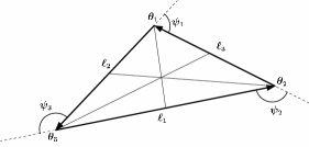
Figure 1: Definition and convention of triangle variables.

Because of translation invariance, the three-point functions depend only on the relative positions of the vertices, so we shall use the three lengths $\psi_{i}$ to specify our oriented triangles.

To define the shear three-point functions we decompose the shear into cross and tangential components in some basis relative to the triangle Zaldarriaga & Scoccimarro (2003); Schneider & Lombardi (2003). This is simpler than trying to find all possible combinations of the three pseudo-vectors $\boldsymbol{\gamma}$ that have non-zero three-point functions, but of course is equivalent. Choosing a basis was “natural” in the case of the two-point function (given by the line joining the two points), but less obvious for a triangle.

Since we are interested in the three-point functions, the knowledge of the position of the points is irrelevant; only their relative positions matters. Therefore, we will drop the vector notation for the vertices $\boldsymbol{\theta}_{i}$. Thus, any configuration is completely described by either the three points relative positions, the three angles or the three side length. Of course, since we have decided to only deal with oriented triangles, the length, and not the side vectors are enough.

A simple solution is to pick some “special” points of the triangle and to project the shear along the vector linking this point and the vertex we are interested in. Note that it is not, in fact, necessary to choose such a special point. Any set of three orientations defined by invariant properties of the configuration will do. In the following, we call this choice of orientation a projection convention. Any change of projection convention can be described by a rotation of each of the projection directions at each vertex of the triangle. Of course, each of these rotations can in principle depend on the shape of the triangle. We will call such change a rotation of the projection convention of angle $(\zeta_{1},\zeta_{2},\zeta_{3})$.

Once the projection convention is chosen, the shear field at the three vertices of the triangle can be decomposed in a tangential and a cross component, $\boldsymbol{\gamma}=(\gamma_{+},\gamma_{\times})$. As in the two point function case, these two components have, respectively, positive and negative parity. This decomposition leads to eight different three-point functions $\gamma_{\mu\nu\rho}$ , $\mu$, $\nu$ and $\rho$ being $+$ or $\times$ . Half of them, $\gamma_{+++}$ and $\gamma_{+\times\times}$ plus permutations are parity positive, whereas $\gamma_{\times\times\times}$ and $\gamma_{\times++}$ plus permutations are of negative parity. Since the three-point functions also depend upon the projection convention, we will sometimes denote them by $\gamma_{\mu\nu\rho}^{(\zeta_{1},\zeta_{2},\zeta_{3})}$, $(\zeta_{1},\zeta_{2},\zeta_{3})$ being a rotation to the reference frame.

We have seen that for the two-point function, parity properties reduce the number of independent functions from four to only two. One can wonder whether the parity properties will also reduce the number of non zero three-point functions. The parity negative two-point functions vanish because after a parity transformation, a simple rotation will bring back the points to the initial position [see Eq. (8)]. This is not the case for three-point functions, except in the special cases of equilateral triangles, and some isoceles configurations, where a rotation can mimic a parity transformation Schneider & Lombardi (2003). This is why in the general case parity-negative three-point functions are non-zero Schneider & Lombardi (2003); Takada & Jain (2003a). Formally a parity transformation of a parity negative three-point function for a configuration $\theta_{1}\theta_{2}\theta_{3}$ gives

$$P\left[\gamma_{\mu\nu\rho}^{(\zeta_{1},\zeta_{2},\zeta_{3})}(\ell_{1},\ell_{2},\ell_{3})\right] = -\gamma_{\mu\nu\rho}^{(\zeta_{1},\zeta_{2},\zeta_{3})}(\ell_{1},\ell_{2},\ell_{3})$$ (14)

$$= \gamma_{\mu\rho\nu}^{(\zeta_{1},\zeta_{3},\zeta_{2})}(\ell_{1},\ell_{3},\ell_{2}),$$

where we have assumed that the transformation exchange the last two vertices. Thus, only if $\ell_{3}=\ell_{2}$, $\zeta_{2}(\ell_{1},\ell_{2},\ell_{3})=\zeta_{3}(\ell_{1},\ell_{2},\ell_{3})$ and $\rho=\nu$, parity forces the three-point function to be zero. Note that for simple projection conventions, the property $\zeta_{2}(\ell_{1},\ell_{2},\ell_{3})=\zeta_{3}(\ell_{1},\ell_{2},\ell_{3})$ will usually be verified.

A free parameter that we overlooked in the case of two-point function is the choice of projection convention. Indeed, we picked the easiest projection where the angles from the reference frame were the same for the two points. If we now allow these two angles to be different, we break the property that the $\langle\gamma_{+}\gamma_{\times}\rangle$ are zero, since we cannot equate parity transformations and $\pi$ rotations, and we are then in similar situation to that of three-point functions. The choice of projection that seemed most natural for the two-point function has this extra property that its parity negative component is zero.

Is it possible to find an analogous “natural” projection convention that reduces the number of non-zero three-point functions? This problem has been partly investigated by Schneider & Lombardi (2003). Here we shall reproduce their results and extend them to answer the question of the preferred projection convention.

In the two-point function cases, as we discussed above, a rotation from the natural projection convention will induce non-zero parity negative part. One can show that the $\xi_{\pm}$ will transform as

$$\xi_{\pm}^{(\zeta_{1},\zeta_{2})}=e^{-i(\zeta_{1}\pm\zeta_{2})}\xi_{\pm}.$$ (15)

In other words, the $\xi_{\pm}$ only acquire a phase, their amplitude is invariant. One can build equivalent “rotational invariant” the three-point functions as described in details in Schneider & Lombardi (2003), where it is showed that any change of the projections axis of the three points will leave the following four complex quantities invariants up to a phase

$$\Gamma_{0}=\left\langle\gamma_{1}\gamma_{2}\gamma_{3}\right\rangle,\,\,\,\,\,\,\,\,\Gamma_{i}=\left\langle\gamma_{i}^{*}\prod_{j\neq i}\gamma_{j}\right\rangle,$$ (16)

with $i=1,2,3$, which can be written as,

$$\Gamma_{\mu}=A_{\mu\nu}\gamma_{\nu}^{\oplus}-i\,\,B_{\mu\nu}\gamma_{\nu}^{\otimes},$$ (17)

where $\mu,\nu=0,1,2,3$ and the matrices $A$ and $B$ have all elements equal to $\pm 1$, $B_{\mu\nu}\equiv 1-2\delta_{\mu\nu}$, $A_{\mu\nu}\equiv B_{\mu\nu}(1-2\delta_{\mu 0})$. In addition, $\gamma^{\oplus}$ and $\gamma^{\otimes}$ denote, respectively, the positive- and negative-parity three-point functions,

$$\gamma^{\oplus}=\left(\begin{array}[]{c}\gamma_{+++}\\ \gamma_{+\times\times}\\ \gamma_{\times+\times}\\ \gamma_{\times\times+}\end{array}\right),\,\,\,\,\,\,\,\,\,\,\gamma^{\otimes}=\left(\begin{array}[]{c}\gamma_{\times\times\times}\\ \gamma_{\times++}\\ \gamma_{+\times+}\\ \gamma_{++\times}\end{array}\right).$$ (18)

The transformation of the $\Gamma_{i}$ under the rotation of the projection directions are given by

$$\Gamma^{\prime}_{0} = \mathrm{e}^{2\mathrm{i}\left(\zeta_{1}+\zeta_{2}+\zeta_{3}\right)}\Gamma_{0}$$ (19)

$$\Gamma^{\prime}_{1} = \mathrm{e}^{2\mathrm{i}\left(-\zeta_{1}+\zeta_{2}+\zeta_{3}\right)}\Gamma_{1}$$ (20)

$$\Gamma^{\prime}_{2} = \mathrm{e}^{2\mathrm{i}\left(\zeta_{1}-\zeta_{2}+\zeta_{3}\right)}\Gamma_{2}$$ (21)

$$\Gamma^{\prime}_{3} = \mathrm{e}^{2\mathrm{i}\left(\zeta_{1}+\zeta_{2}-\zeta_{3}\right)}\Gamma_{3}.$$ (22)

This property has some interesting consequences. Indeed, Eqs. (19-22) show that projection convention rotations will not change the modulus of the $\Gamma_{i}$. At most, if a preferred projection exists (i.e. if the eight three-point functions are redundant), they can be reduced to four quantities. It might be possible that for a given triangle shape one can find a preferred convention projection for which all parity-negative three-point functions will be zero (one of course can always find a rotation that yield three vanishing three-point functions). Let us note $(\zeta_{1},\zeta_{2},\zeta_{3})$ the rotation that will transform a given projection convention into the projection we are looking for. Eqs (19-22) define a system of four equations that our $\zeta_{i}$ have to verify. This is possible if and only if $\Phi_{i}$, the phases of the $\Gamma_{i}$, verify the relation

$$\Phi_{0}=\Phi_{1}+\Phi_{2}+\Phi_{3}+k\pi\>k\epsilon\mathbb{Z}.$$ (23)

For isosceles triangles, this condition can be shown to be true. Indeed, the parity properties imply that for any isoceles configuration in $\theta_{1}$, the following relations hold

$$\Gamma_{2} = \Gamma_{3}^{*}$$ (24)

$$\Gamma_{1} = \Gamma_{1}^{*}$$ (25)

$$\Gamma_{0} = \Gamma_{0}^{*},$$ (26)

that is, $\Phi_{0}$ and $\Phi_{1}$ are zero (modulo $\pi$), whereas $\Phi_{2}=-\Phi_{1}$. The rotations that change a projection convention to one with the zero parity negative three-point functions are of the form $(0,-\Phi/4,\Phi/4)$, where $\Phi=\Phi_{2}=-\Phi_{3}$ is the phase in the first projection convention. Note that this result is of little use, since it just shows in a different language that only four quantities are needed to describe the isosceles configurations, which can be shown only from parity considerations. Moreover, the phase $\Phi$ has to be evaluated in order to find the preferred convention projection.

Neither parity properties, nor geometrical considerations allow us to prove or disprove the conditions in Eq. (23) in the general case. The answer to our question will have to come from the computation of the three-point functions that we will exhibit in the next section.

3 Analytical predictions for the three point functions

We now proceed to calculate the eight shear three-point functions. This can be done in terms of the eight $\gamma_{\mu\nu\rho}$ or four $\Gamma_{i}$ which are completely equivalent. In fact we will present results in both representations, although most of the time we deal with $\Gamma_{i}$.

To compute the three point functions of the shear, we will use a simple model that captures most of the features of a more detailed calculation. The reason for studying such a simplified model will become clear in section 4 when we discuss how to “optimally” combine the eight three-point functions into a single three-point function.

3.1 A single halo

Weak lensing surveys provide their best constraints at scales small enough (one to ten arc minutes) that are well into the non-linear regime. For example, for measurements on background galaxies at redshift around unity, the weak lensing efficiency is maximum at about $z=0.43$ for an $\Omega_{m}=0.3$, $\Omega_{\Lambda}=0.7$ cosmology, for which one arc minute corresponds to a distance of 0.3 Mpc/h. For such scales, contributions to lensing statistics come mainly from light deflection by single dark matter halos, and it is a good approximation to compute the light deflection ignoring coupling between different deflections Cooray & Hu (2002); Van Waerbeke et al. (2001). In the language of the so-called halo model Cooray & Sheth (2002), statistics are dominated by the “one-halo” contribution, and this has been verified for the shear three-point functions by comparison with measurements in numerical simulations Takada & Jain (2003a, c). Remarkably, as shown in Zaldarriaga & Scoccimarro (2003), for scales of about three arc minutes the full dependence of the shear three-point functions on the triangle shape for the halo model agree very well with a calculation based on a singular isothermal sphere up to an overall amplitude. Given these results, we will only slightly go beyond the singular isothermal model. We shall assume that the shear three-point functions can be calculated by the contribution from one spherical halo located at the maximum of the lensing efficiency window. The halo profile will be taken as a general power-law

$$\rho(r)\propto\frac{1}{r^{n}},$$ (27)

where $n=2$ corresponds to an isothermal sphere. In general, simulations suggest dark matter halos have $n\sim 1$ near the halo center and $n\sim$3 at large distances Navarro et al. (1997),

$$\rho\propto\frac{1}{r(r_{o}+r)^{2}},$$ (28)

where the effective profile index is $n_{\textrm{eff}}=2$ when $r=r_{o},$typically a tenth of the halo virial radius. Assuming a fixed $n$ (which can be determined by the angular scale probed and the halo mass of the dominant contribution to the three-point function) we loose cosmological information, but on the other hand the calculation can be done analytically and also the scaling properties of Eq. (27) allows us to ignore the halo profile normalization and the effects of projection which enter as an overall constant.

Computing lensing by a spherical halo is very simple. From Eqs. (1), (3) and (27) it follows that the shear pattern behaves as

$${\boldsymbol{\gamma}}=\left[\begin{array}[]{c}\cos(2\theta)\\ \sin(2\theta)\end{array}\right]\gamma(r),$$ (29)

with

$$\gamma(r)=r^{1-n}.$$ (30)

The contribution of such a halo to the three-point functions is therefore

$$\gamma_{\mu\nu\rho}(\ell_{1},\ell_{2},\ell_{3}) =$$

$$\int\mathrm{d}^{2}u\;\boldsymbol{P}_{\mu}\cdot\boldsymbol{\gamma}(\boldsymbol{\theta_{1}})\,\boldsymbol{P}_{\nu}\cdot\boldsymbol{\gamma}(\boldsymbol{\theta_{2}})\,\boldsymbol{P}_{\rho}\cdot\boldsymbol{\gamma}(\boldsymbol{\theta_{3}}),$$

where the symbols $\boldsymbol{P}_{\mu}$ stand for the projectors in the $+$ and $\times$ directions. The three points are taken at the positions $\boldsymbol{\theta}_{i}$, such that $\boldsymbol{\ell}_{i}=\boldsymbol{\theta}_{i+1}-\boldsymbol{\theta}_{i+2}$, and we use all our indices $i$ modulo 3. Note that we integrate out the position of the center of the halo, denoted by $\boldsymbol{u}$.

Equations (30) and (3.1) imply that in our simple model, the following scaling relationship holds,

$$\gamma_{\mu\nu\rho}(\lambda\,\ell_{1},\lambda\,\ell_{2},\lambda\,\ell_{3})=\lambda^{5-3n}\,\gamma_{\mu\nu\rho}(\ell_{1},\ell_{2},\ell_{3}).$$ (32)

Since all choices of projections are equally valid, we can choose here the projection operator to simplify the calculation as much as possible. Here we will take the projection direction at each vertex to be that of the opposite side. Note that this is equivalent, up to a sign, to projecting along the lines joining each vertex of the triangle to its orthocenter Schneider & Lombardi (2003). For simplicity, we shall refer to our projection as “orthocenter”. With this choice, the projected shear reads

$$\boldsymbol{P}_{\mu}\cdot\boldsymbol{\gamma}(\boldsymbol{\theta_{i}})=\frac{\mathrm{trig}_{\mu}(2\phi_{i})}{\left|\boldsymbol{\theta}_{i}-\boldsymbol{u}\right|^{n-1}},$$ (33)

where $\mathrm{trig}_{+}\equiv\cos$ and $\mathrm{trig}_{\times}\equiv\sin$. The angle $\phi_{i}$ is the angle defined by the line joining the vertex and the center of the halo and the opposite side of the vertex

$$\cos(\phi_{i})=\frac{\left(\boldsymbol{u}-\boldsymbol{\theta}_{i}\right)\cdot\boldsymbol{\ell}_{i}}{\left|\boldsymbol{u}-\boldsymbol{\theta}_{i}\right|\ell_{i}}.$$ (34)

Given our choice of projection, the trigonometric functions can be written in terms of the configuration $(\ell_{1},\ell_{2},\ell_{3})$, and the relevant integrals computed in terms of hypergeometric functions (see Zaldarriaga & Scoccimarro (2003) for description of the integration procedure). We refer the reader to Appendix A for details.

3.2 Results

Figures 2, 3 and 4 present our basic results for the isothermal profile case ($n=2$), for fixed ratios of sides ($\ell_{2}/\ell_{3}=1,2,3$), as a function of angle $\psi_{1}$ as defined in Fig. 1. Due to the scaling in Eq. (32) a choice of sides ratio completely describes other triangles with different overall scale up to a normalization constant. Figure 2 shows $\gamma_{\mu\nu\rho}$, whereas Figs. 3 and 4 show $\Gamma_{i}$. A comparison between different values of the power-law index $n$ is presented in Figs. 5 for $\Re(\Gamma_{0})$ and $\Im(\Gamma_{2})$ when $\ell_{2}=\ell_{3}$.

Figures 2 and 3 show results in two different projection conventions. To go from the orthocenter to the center of mass projection convention it is necessary to compute the angles $\eta_{i}$ between the line joining the center of mass with the $i^{\textrm{th}}$ vertex and the $\ell_{i}$ (see Fig. 1) and use the relations given by Eqs. (19-22). Comparing both projections is useful to disentangle geometrical properties from projection-dependent behavior. Comparing top and bottom panels in Figs. 2 and 3 we see that, qualitatively, the orthocenter projection leads to “wigglier” correlation functions.

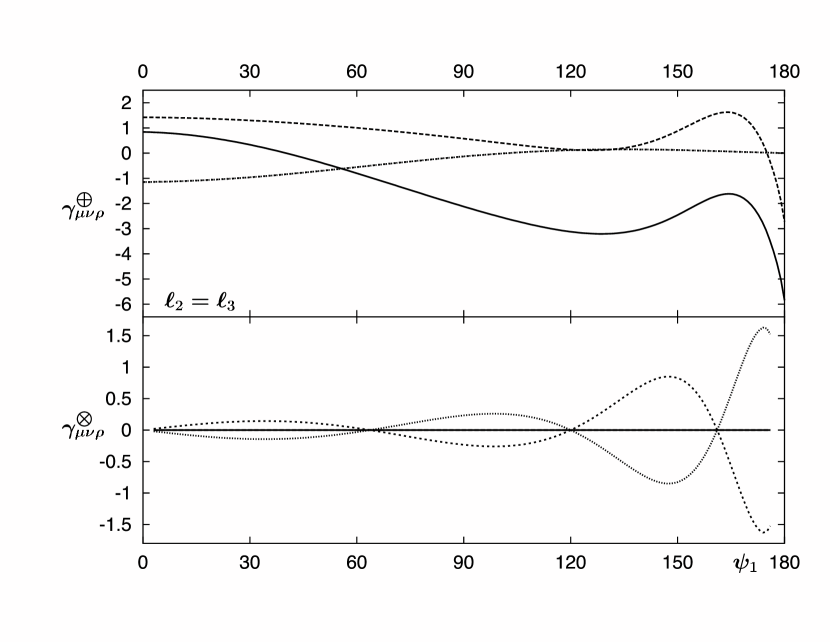
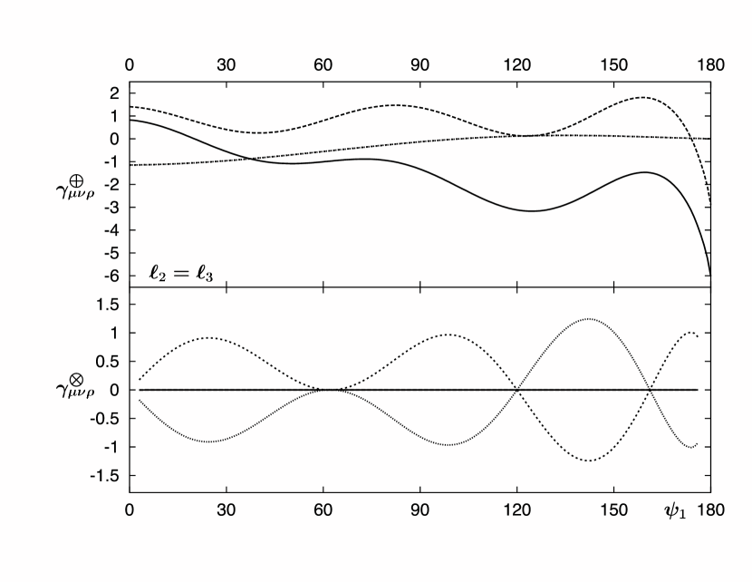
Figure 2: The top (bottom) panel shows the positive ($\gamma_{\mu\nu\rho}^{\oplus}$) and negative ($\gamma_{\mu\nu\rho}^{\otimes}$) parity three-point functions for the center of mass (orthocenter) projection convention. We have assumed an isothermal sphere profile ($n=2$) and a fixed ratio ($\ell_{2}/\ell_{3}=1$) and plotted as a function of the angle $\psi_{1}$ (see Fig. 1 for a definition).Line styles for parity positive three-point functions are $\gamma_{+++}$ (solid), $\gamma_{+\times\times}$(long-dashed), $\gamma_{\times+\times}$ (dotted) and $\gamma_{\times\times+}$ (dashed) whereas for negative parity $\gamma_{\times\times\times}$ (solid),$\gamma_{\times++}$ (long-dashed),$\gamma_{+\times+}$ (dotted) and $\gamma_{++\times}$ (dashed).

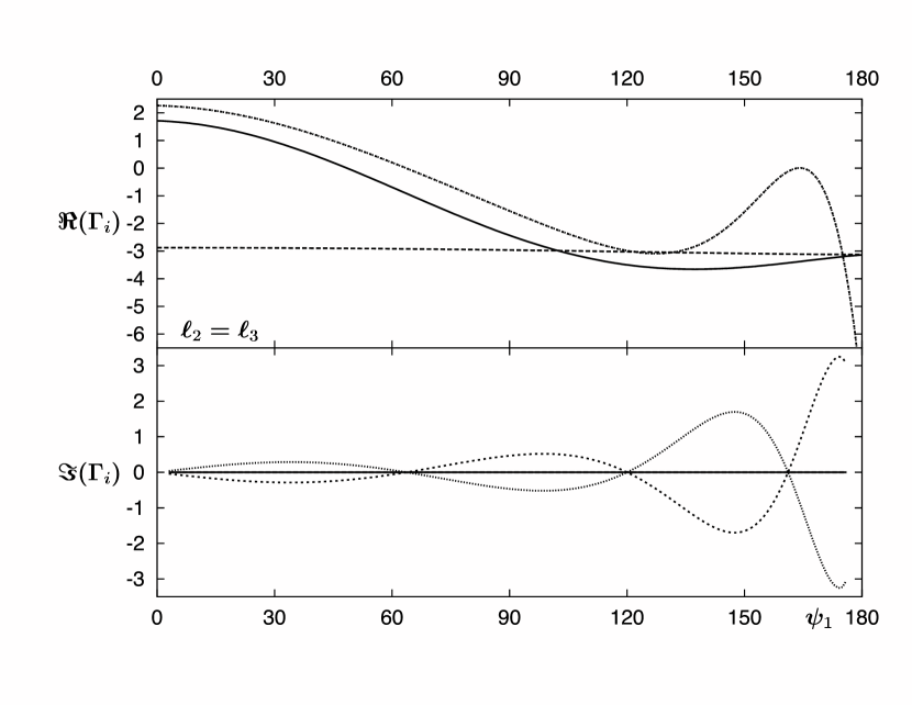
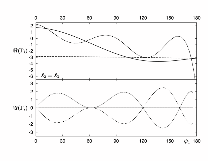
Figure 3: Same as Fig. 2 but for the real (positive-parity) and imaginary (negative parity) parts of $\Gamma_{i}$. Line styles are as follows: $\Gamma_{0}$ (solid), $\Gamma_{1}$ (long-dashed), $\Gamma_{2}$ (dotted), $\Gamma_{3}$ (dashed).

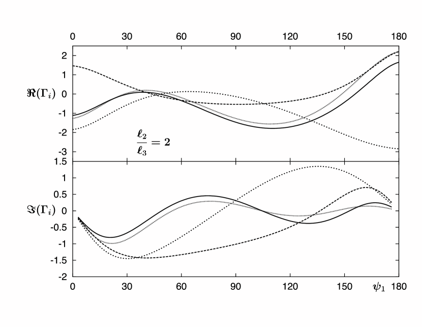
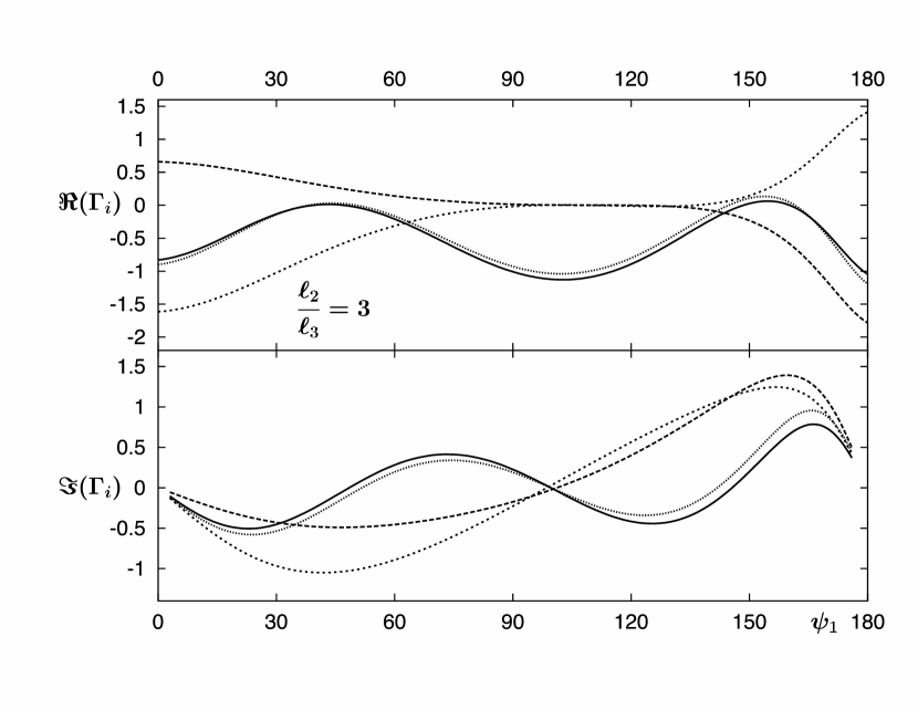
Figure 4: Same as Fig. 3 but only in the center of mass projection, for sides ratio $\ell_{2}/\ell_{3}=2$ (top panel) and $\ell_{2}/\ell_{3}=3$ (bottom panel).

Parity related features in the three-point functions for isoceles triangles are evident: $\gamma_{\times+\times}=\gamma_{\times\times+}$ , $\gamma_{++\times}=-\gamma_{+\times+}$ and $\gamma_{\times\times\times}=\gamma_{\times++}=0$ in fig 2 and $\Gamma_{2}=\Gamma_{3}^{*}$ and $\Im(\Gamma_{0})=\Im(\Gamma_{1})=0$ in fig 3. Furthermore, for equilateral triangles $\gamma_{+\times\times}=\gamma_{\times+\times}=\gamma_{\times++}$ and $\gamma_{\times++}=\gamma_{+\times+}=\gamma_{++\times}=0$. Other features that these figures show appear more difficult to predict; for example, the local extrema of $\gamma_{+++}$ for configurations close to equilateral triangles are not exactly located at $2\pi/3$ and depend on the projection convention (after all, the average over the position of the halo does depend on projection convention). In addition, points where some $\gamma_{\mu\nu\rho}$ are equal to each other change location (and can disappear or appear) as projection convention is changed.

Figure 4 shows what happens as we consider triangles other than isosceles. Note that now all the parity-negative three-point functions are non-zero. The fact that $\Gamma_{1}\sim-\Gamma_{2}^{*}$ (and accordingly that $\Gamma_{0}\sim\Gamma_{3}$) can be understood as follows. Indeed, when $\cos(\pi-\psi_{1})=1/4$ ($1/6$ for bottom panel) the configuration is isoceles in $\theta_{3}$, thus ensuring that $\Gamma_{1}=\Gamma_{2}^{*}$ by parity. Around this angle, it follows from parity that $\Gamma_{2}(\psi_{1}+\epsilon,\ell_{2},\ell_{3})\sim\Gamma_{1}^{*}(\psi_{1}-\epsilon,\ell_{2},\ell_{3})$ for $\epsilon\ll\ell_{2}/\ell_{3}$. In addition, as $\ell_{2}/\ell_{3}$ increases, the product $\gamma_{1}\gamma_{2}$ will start to dominate the three-point function, and thus parity properties become essentially those of the two-point function, insuring that $\Gamma_{1}\sim-\Gamma_{2}^{*}$. These arguments explain why as $\ell_{2}/\ell_{3}$ increases (compare top and bottom panels in Fig. 4) $\Gamma_{1}$ gets closer to $-\Gamma_{2}^{*}$ and $\Gamma_{0}$ to $\Gamma_{3}$.

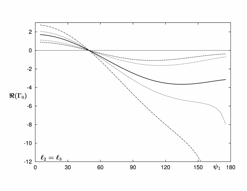
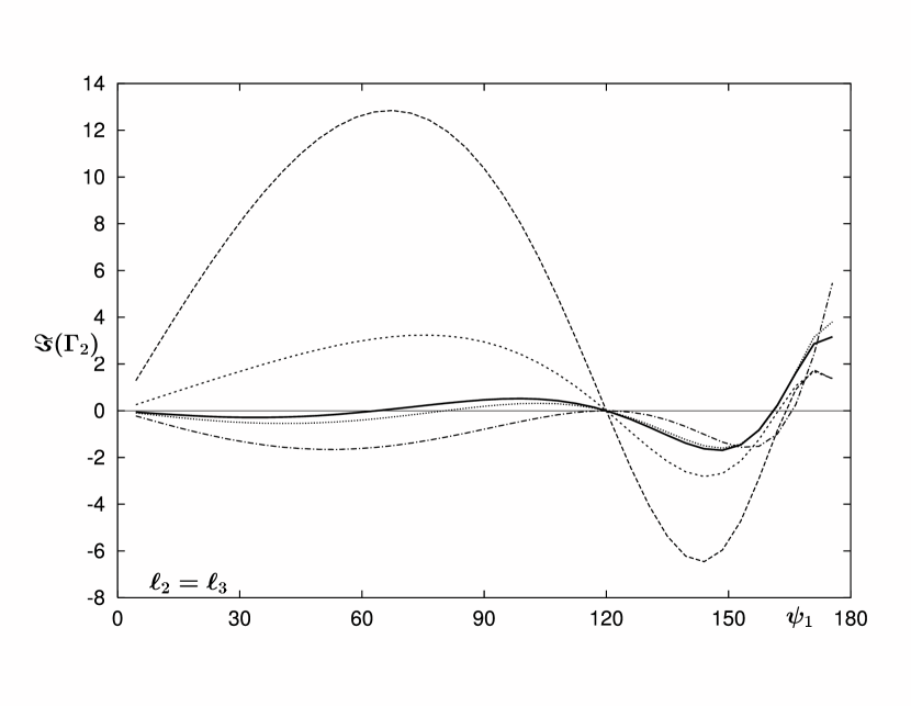
Figure 5: The real part of $\Gamma_{0}$ (top) and the imaginary part of $\Gamma_{2}$ (bottom) for different values of the profile index of the halo $n$ and $\ell_{2}=\ell_{3}$. Line styles are $n=1.2$ (long-dashed), $n=2$ (solid), $n=2.1$ (dotted), $n=2.5$ (dot-dashed)

Figure 5 shows how the correlation function $\Re(\Gamma_{0})$ and $\Im(\Gamma_{2})$ depend on the slope of the profile $n$. The zero crossing of $\Im(\Gamma_{2})$ at $2\pi/3$ can be explained by parity; however, the other zero crossings (and the number of them) depend on the profile slope $n$. For $\Re(\Gamma_{0})$ there is a zero crossing at $\psi_{1}\sim 50^{o}$, which appears robust to changes in $n$, but we found no simple explanation for this.

We now consider again the question raised at the end of section 2.3 regarding the existence of a preferred projection, in the context of our simple model. The condition in Eq. (23) can be rewritten as

$$\daleth=\Gamma_{0}\left(\Gamma_{1}\Gamma_{2}\Gamma_{3}\right)^{*}\epsilon\leavevmode\nobreak\ \mathbb{R}.$$ (35)

Figure 6 shows $\Re(\daleth)$ and $\Im(\daleth)$ for triangle with $\ell_{2}/\ell_{3}=2$. We see from the bottom panel that the imaginary part does not vanish, thus it is not possible to find a preferred projection where all negative-parity three-point functions vanish [but of course we can make three of them vanish by using Eqs. (19-22)]. Note however, that the relation in Eq. (35) is close to being satisfied, at least approximately, for almost all $\psi_{1}$.

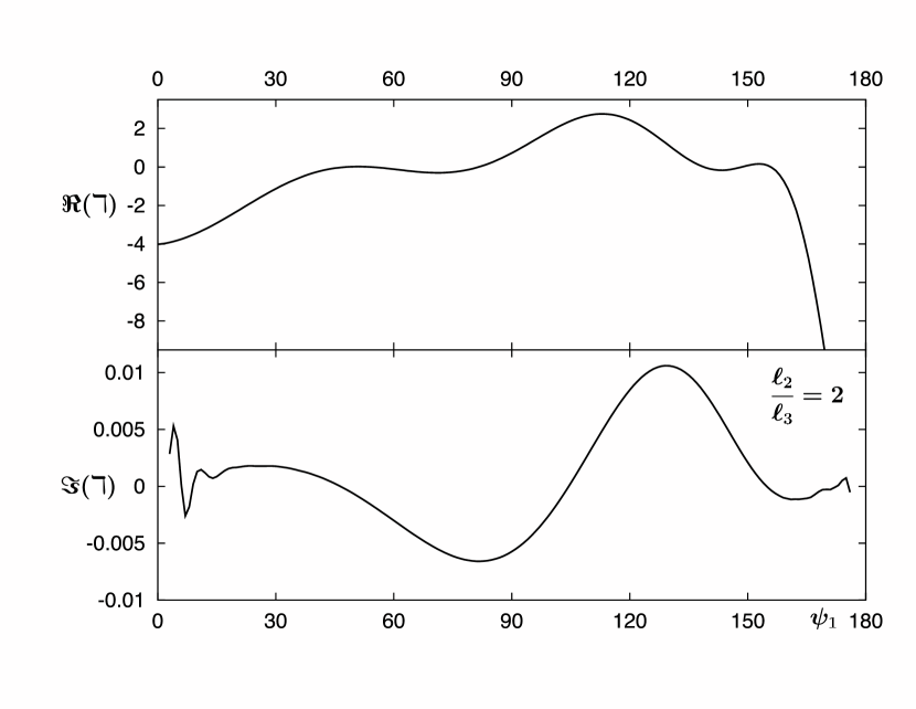
Figure 6: The real (top) and imaginary part of $\daleth$ for the $\ell_{2}/\ell_{3}=2$ case as a function of $\psi_{1}$. The non-zero imaginary part shows that there is no preferred projection convention where all negative-parity three-point functions vanish.

4 The shear three-point functions in numerical simulations

We now describe the results of measuring the shear three-point function in N-Body simulation. For details about the simulations and the procedure we followed to make the measurements see Appendix B. Basically, we created shear maps with three different resolutions that cover a large range of scales (roughly from 4 arc seconds up to 1, 10 and 40 arc minutes). In practice, we measured the $\gamma_{\mu\nu\rho}$ in the center of mass projection convention, and then transformed to the $\Gamma_{i}$.

4.1 Results

We start by comparing the scaling of the three-point functions to see, using Eq. (32), whether the effective value of the profile index is reasonable compared to expectations based on dark matter halo profiles such as Eq. (28). Figure 7 shows results from the medium resolution measurements, where we have scaled $\Re(\Gamma_{1})$ assuming an $n=2$ profile. More precisely, given an isosceles triangle where two sides are equal to $\ell$, we have fitted for $\bar{\Gamma_{1}}$ and $\alpha(\ell)$ so that

$$\Re(\Gamma_{1}(\psi_{1},\ell,\ell))\sim\bar{\Gamma_{1}}(\ell)(1+\alpha(\ell)\psi_{1}),$$ (36)

where $\alpha(\ell)$ incorporates the dependence on the angle between the two equal sides. In practice we found that variations of $\alpha$ with $\ell$ are small, thus they have been neglected. To avoid artificial deviations from scaling due to our binning (see discussion below), we have kept our triangles far enough from being collapsed, i.e. we restrict $\pi/9\leq\psi_{1}\leq 8\pi/9$. The results in Fig. 7 show that the scaling between $1$ and $3$ arc-min is consistent with that of an isothermal sphere, whereas for larger angular scales $\ell\bar{\Gamma_{1}}(\ell)\sim\ell^{-1}$ and thus the effective profile index increases toward $n=7/3\sim 2.3$ [see Eq. (32)]. This is consistent with the hypothesis that we are only sensitive to the index of halos that contribute the most at the scale we are probing. Indeed, at the maximum of the lensing window function, $z\sim 0.4$, masses in the range $10^{13}M_{\odot}$ to $10^{15}M_{\odot}$ have $r_{0}$ [where $n_{\textrm{eff}}=2,$ see Eq. (28)] of the order of a few arc-minutes.

Given the results in Fig. 7, we can now compare the $n=2$ model to our measurements in simulations at arc minute scales to check whether they agree (up to an arbitrary constant that our model does not predict). Figure 8 shows the comparison between the $n=2$ model (with amplitude fixed by maximizing agreement with $\Gamma_{2}$) and simulations for triangles with $\ell_{2}=\ell_{3}=2.25$ arc-minutes. We see that by adjusting a single amplitude, all other $\Gamma_{i}$ show good agreement as well, giving support to our simple model. This result is not surprising given that an isothermal profile was shown to agree with a calculation based on the halo model in Zaldarriaga & Scoccimarro (2003), and the latter was found to be in good agreement with measurements in numerical simulations in Takada & Jain (2003a, c).

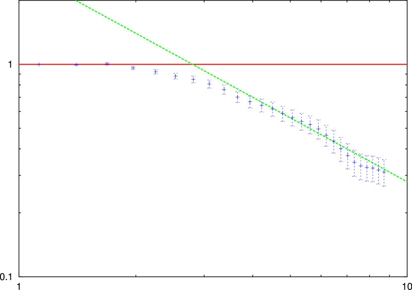
Figure 7: Scaling test for $\ell_{0}=1.125^{\prime}$. The points with error bars represent $S=\bar{\ell\Gamma_{1}}(\ell)/(\ell_{0}\bar{\Gamma_{1}}(\ell_{0}))$. The solid line is $S=1$ ($n=2$), whereas the dotted line denotes to which according to Eq. (32) correspond to $n\simeq\approx 2.3$.

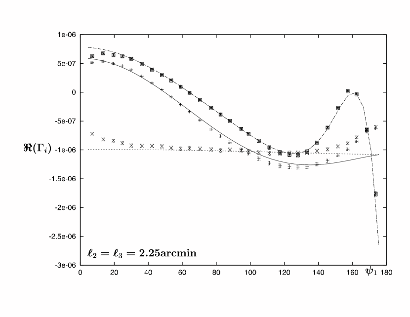
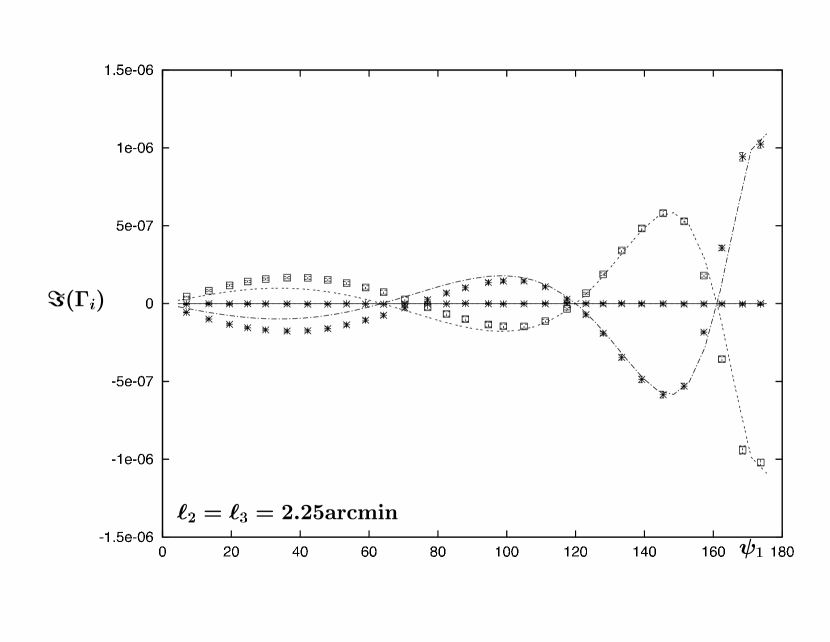
Figure 8: Predictions from our $n=2$ model compared against measurements in simulations for isosceles triangles with $\ell=2.25$ arc minutes. The top (bottom) panel shows the real (imaginary) part of $\Gamma_{1}$, and the model arbitrary amplitude has been adjusted to match $\Gamma_{2}$.

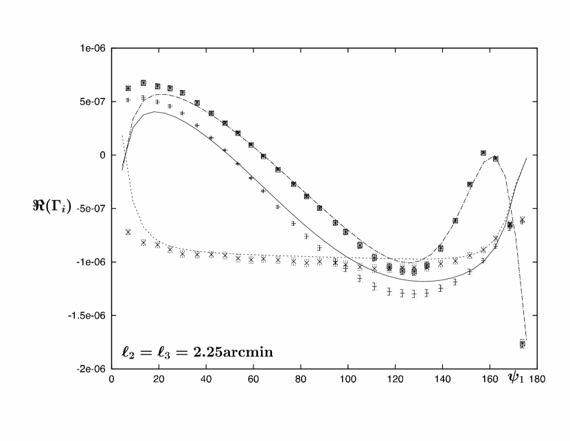
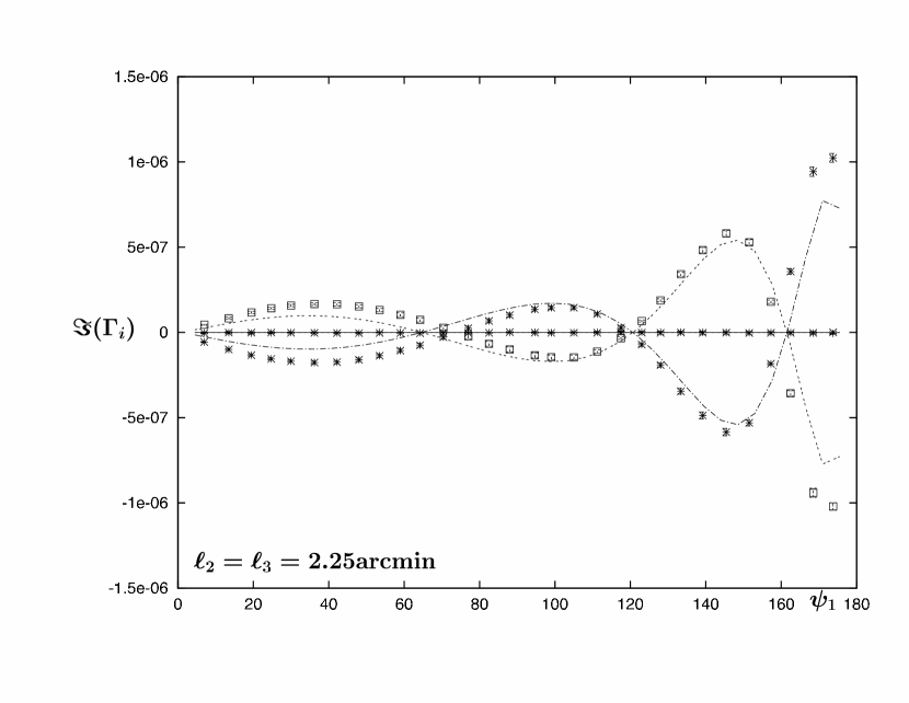
Figure 9: Same as previous Figure, but modifying the model prediction to mimic the effect of binning in the simulations, approximately, as in Eq. (37).

It is apparent from Fig. 8 that as the triangle becomes collapsed ($\psi_{1}\rightarrow 0^{o},180^{o}$) the agreement with the model is not as good, particularly in the parity positive case. This can be understood as a result of the effect of binning in the simulation measurements, where many configurations contribute to each bin. In the case we are considering here, it amounts to an error of order 10% on the length of $\ell_{2}$ and $\ell_{3}$ and about 2% on the angle $\psi_{1}$. On can estimate the effect of binning by computing in our model $\tilde{\Gamma_{i}}$ defined as instead

$$\tilde{\Gamma}_{i}=\frac{\Gamma_{i}(\psi_{1},(1+\epsilon)\ell,\ell)+\Gamma_{i}(\psi_{1},\ell,(1+\epsilon)\ell)}{2},$$ (37)

with $\epsilon=\Delta\ell/\ell\sim 0.1$. This prediction is compared to the same measurements in Fig. 9. The results show that the behavior near collapsed triangles, such as the sharp divergence of $\Re(\Gamma_{1})$, can be explained by the discreteness error due to binning. Generically, our model shows that the effect of a small error in the determination of the length of the triangle sides can translate into significant corrections to the three-point functions for nearly collapsed triangles. Another noticeable discrepancy between our model and the numerical simulations are the slightly displaced zeros of $\Im(\Gamma_{2})$ and $\Im(\Gamma_{3})$ and their amplitudes for $\psi_{1}<60^{o}$. The former can be improved by slightly changing the profile index, as shown in Fig. 5 the first zero in these three-point functions is very sensitive to small variations in the profile index. The difference in amplitude can also be seen in similar plots in Takada & Jain (2003a) when using the full halo model; this suggests perhaps that such deviations could be due to the assumption of spherical halos. It is worth exploring this issues further as they may provide a novel way of testing dark matter halo profiles and shapes. Some steps in this direction have been already taken in Takada & Jain (2003c), where the two- and three-point function of the convergence field were used to constrain parameters of halos such as concentration and inner profile slope.

Finally, we present results from simulations for isosceles and non-isosceles configurations, from our high resolution measurements, at $\ell_{2}=0.42^{\prime}$ (Fig. 10) and middle resolution one at $\ell_{2}=2.8^{\prime}$ (Fig. 11). These should be compared with the top panel in Fig. 3 for the isosceles case, and Fig. 4 for non-isosceles triangles. We can see that for $\ell_{2}=2.8^{\prime}$ the agreement with Figs. 3-4, as expected from the scaling test that suggests that the effective index is close to n = 2. However, for $\ell_{2}=0.42^{\prime}$ we see that there are significant differences, the three-point functions changed as expected from the results of our analytical model in Fig. 5 when the profile index becomes smaller than $n=2$.

We have also made measurements in lower resolution sets (not presented here) that allows us to probe larger scales. Again we see consistent results with those expected from Fig. 5 for indices $n>2$, in particular regarding the dependence of number of zeros as the scale is changed. However, one cannot extend this study to significantly larger scales, as contributions from more than a single halo become important and our simple model breaks down.

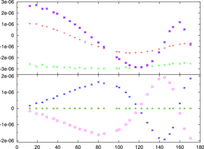
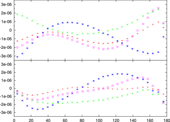
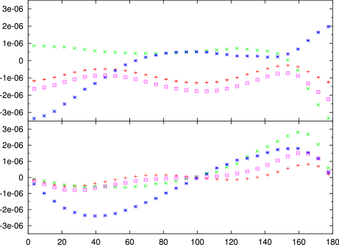
Figure 10: $\Gamma_{i}$ measured for $\ell_{2}=0.42^{\prime}$. In each panel top (bottom) part shows positive (negative) parity three-point functions. Panels correspond to isoceles triangles (top), $\ell{}_{2}=2\ell_{3}$ (middle) and $\ell_{2}=3\ell_{3}$ (bottom). Symbols are as follows $\Gamma_{0}$ (plus),$\Gamma_{1}$ (cross), $\Gamma_{2}$ (star) and $\Gamma_{3}$ (box).

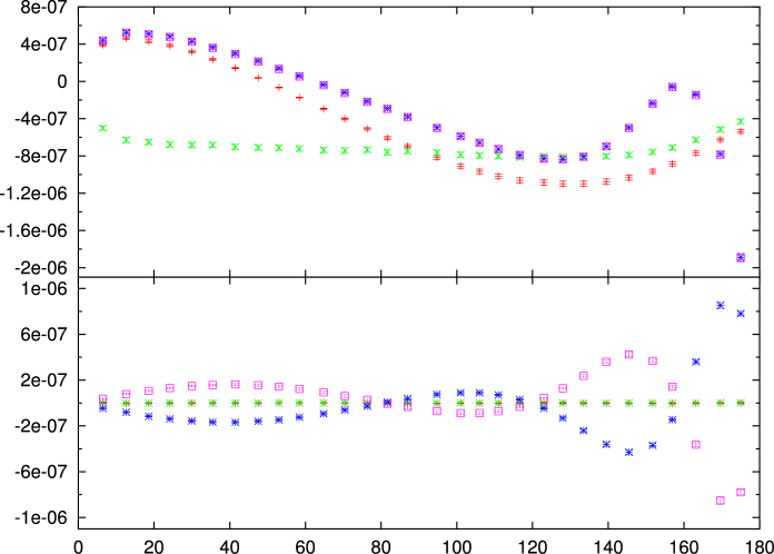
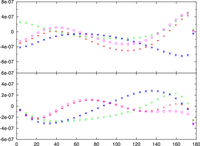
Figure 11: Same as previous Figure for $\ell_{2}=2.8^{\prime}$.

5 Estimators of cosmic shear three-point functions

We now turn to the problem of building a simpler estimator of the shear three-point function. One obvious solution is to combine them to reconstruct the weak lensing convergence bispectrum Schneider et al. (2005). However, equations involved into the computation of the bispectrum from the shear three-point functions are very difficult to compute numerically. They correspond to the inversion of a non-local equation; a task that usually cannot be fulfilled from real data without some regularization of the problem.

The so-called $M_{ap}$ statistic filters provide such regularization. They have been used successfully to reconstruct the filtered convergence two-point function from measurement of the shear two-point functions Schneider et al. (2002). Another great advantage of these family of compensated filters is that, to some extent, they can be custom designed to have a finite real space support (or at least exponentially small wings), allowing for relatively quick data analysis. A problem of those method, however, is that one can expect a degraded signal to noise from the initial data, due to the use of compensated filters that impose cancellation of part of the signal. This have not been an important issue for two-point functions.

The $M_{ap}$ approach has been also applied to three point functions Jarvis et al. (2004); Pen et al. (2003); Schneider et al. (2005). It has been showed that one can exhibit a summation procedure for measured data that results into an estimation of the $M_{ap}$ filtered bispectrum of the convergence field. Measurements on real data have been performed. The quality of data being low and the degradation of the signal-to-noise ratio inherent to $M_{ap}$ statistics results in very large error-bars Jarvis et al. (2004); Pen et al. (2003).

Owing to its simple relation with the convergence bispectrum and thus to the matter distribution bispectrum, the $M_{ap}$ approach is certainly a very appealing estimator of the weak lensing three-point function. However, as it seems to require a high quality dataset, the need for a simple and robust estimator of the weak-lensing three-point function remains. The shear three-point functions $\Gamma_{i}$ can provide such tool, but they still have a complicated dependency on the configuration. Our goal in this section, is to use our analytical prescription in order to propose a way to build an estimator with simpler properties, yet avoiding as much as possible cancellations to preserve the signal-to-noise ratio.

5.1 Previous estimators

Bernardeau, van Waerbeke and Mellier Bernardeau et al. (2003) (hereafter BvWM) proposed a simple estimator that exhibits some of the properties discussed above. They studied the pseudo vector field $\boldsymbol{\mathcal{F}}$

$$\boldsymbol{\mathcal{F}}(\ell_{1},\ell_{2},\ell_{3})=\left\langle\boldsymbol{\gamma}_{1}\left(\boldsymbol{\gamma}_{2}\cdot\boldsymbol{\gamma}_{3}\right)\right\rangle,$$ (38)

where all pseudo vectors $\boldsymbol{\gamma}$ are projected along the direction given by $\boldsymbol{\ell}_{1}$. In such case, symmetry does not imply that $\mathrm{\mathcal{F}}$ vanishes. BvWM were able to evaluate $\mathcal{F}$ for special configurations of the three points. They also computed it in the framework of the hierarchical ansatz and measured it in N-body simulations. From their results, it seemed that the parity-negative part of $\boldsymbol{\mathcal{F}}$ was negligible and that the parity-positive part was not changing sign in a small region around $\theta_{2}\theta_{3}$. They empirically fitted the shape of this region by an ellipse of focal points $\theta_{2}$, $\theta_{3}$. In light of this, they proposed to use the averaging on the ellipse of the parity positive component of $\boldsymbol{\mathcal{F}}$ as their estimator of the shear three point function.

The pseudo-vector $\mathcal{F}$ can be re-expressed as a combination of the $\Gamma_{i}$. Let us place ourselves in the projection convention defined by the direction of $\theta_{2}\theta_{3}$ (this choice of projection is peculiar in the sense that it artificially breaks the symmetry properties by distinguishing one of the points). With this choice, the scalar product $\left(\boldsymbol{\gamma}_{2}\cdot\boldsymbol{\gamma}_{3}\right)$ reads

$$\left(\boldsymbol{\gamma}_{2}\cdot\boldsymbol{\gamma}_{3}\right)=\gamma_{(2)+}\gamma_{(3)+}+\gamma_{(2)\times}\gamma_{(3)\times}.$$ (39)

Multiplying the previous Eq. by $\gamma_{1}$ leads to the expression of $\boldsymbol{\mathcal{F}}$

$$\boldsymbol{\mathcal{F}}=\left(\begin{array}[]{l}\gamma_{+++}+\gamma_{+\times\times}\\ \gamma_{\times++}+\gamma_{\times\times\times}\end{array}\right),$$ (40)

which can be written in terms of the $\Gamma_{i}$

$${\mathcal{F}}=\frac{1}{2}\left(\Gamma_{2}+\Gamma_{3}\right).$$ (41)

Remember that the last equation holds only for the $\theta_{2}\theta_{3}$ projection convention; Eqs. (19-22) can be used to rotate the expression into some other projection convention.

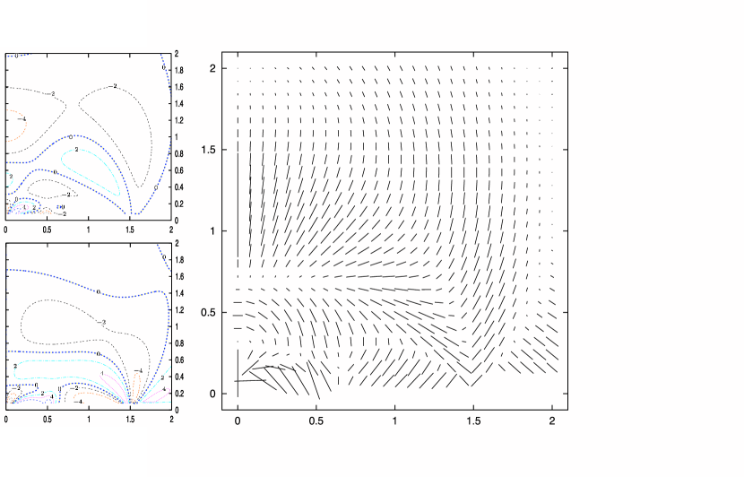
Figure 12: Predictions for the $\boldsymbol{\mathcal{F}}$ estimator. Left panel presents the real/parity positive (top) and imaginary/parity negative (bottom) parts. Right panel shows the resulting pattern. The points $\theta_{2}$ and $\theta_{3}$ are fixed to $(0,-1/2)$ and $(0,1/2)$. The coordinate gives the position of $\theta_{1}$. We only shows one fourth of the plane. The rest of it can be determined from parity properties. ${\mathcal{F}}_{\times}$ goes go to zero on the x and y axis.

Figure 12 presents the $\boldsymbol{\mathcal{F}}$ pseudo-vector in the top right quadran of the plane, computed from our analytic model, with index $n=2$. The base of triangle $(\theta_{2}\theta_{3})$ spans the range $[-1/2,1/2]$ on the x axis. Fig. 12 partly reproduce the result from Bernardeau et al. (2003). In particular, even if the parity-negative part of the pseudo-vector ${\mathcal{F}}$ is smaller than the parity positive component, it is not negligible. We also explore the region where the parity positive component keeps the same sign. Contour plots on the left panels of Fig. 12 shows that its shape is richer than that of an ellipse. Changing the profile index $n$ modifies slightly the properties of $\boldsymbol{\mathcal{F}}$. The overall shape shown Fig. 12 is conserved. Modifications are concentrated around the $x$ axis, when the configuration is nearly flat; in particular, the number of constant sign region along $y_{\theta_{1}}=0$ changes as can be expected from Fig. 5. Finally, the amplitude of the parity-negative component decreases slightly when the value of the profile index increases. This explains the apparent discrepancy between BvWM results and ours. They are averaging their measurement in numerical simulations on scales bigger that the one probing the region where the halo profile is well described by $n=2$. Moreover, the binning procedure can average out the parity negative part.

Although ignoring the parity negative part and summing the parity positive part over an ellipse is a good starting point, the BvWM estimator can be improved by using the prediction of the expected shear pattern as we now discuss.

5.2 A new estimator: projecting measurements onto shear pattern templates

An approach to avoid signal to noise cancellation due to positive and negative contributions when combining different three-point functions is to “project” the measurements of the $\Gamma_{i}$ directly onto the expected result (template) from analytic predictions and build an estimator such as

$$\mathcal{D}_{0}\equiv\sum_{i}\tilde{\Gamma_{i}}\Gamma_{i}^{*},$$ (42)

$\tilde{\Gamma_{i}}$ being the analytical predictions, the star denoting the complex conjugate. Note that $\mathcal{D}_{0}$ now depends on our choice of profile index $n$. One can do even better, assuming that the covariance of the $\Gamma_{i}$ is known, by building a “minimum variance” estimator of the three-point function

$$\mathcal{D}_{1}\equiv\sum_{i,j}\tilde{\Gamma_{i}}\left\langle\Gamma_{i}\Gamma_{j}^{*}\right\rangle^{-1}\Gamma_{j}^{*},$$ (43)

where $\left\langle\Gamma_{i}\Gamma_{j}^{*}\right\rangle^{-1}$ denotes the inverse of the covariance matrix. $\mathcal{D}_{1}$ is only a minimum variance estimator to the extent that its distribution can be approximated to be Gaussian.

It has been shown that to a good approximation, the covariance of the three-point function of the weak lensing shear can be evaluated by restricting the computation to the Gaussian contribution Takada & Jain (2003c). However, even if we restrict ourselves to the Gaussian contribution, the covariance matrix is difficult to compute analytically. Indeed, as discussed above the geometrical properties of the shear complicate the calculation of the three-point functions, and the situation is even worse here, as we have to integrate over all possible orientations and positions of two identical triangles. To avoid such complication, we evaluate the covariance matrix by measuring it in our numerical simulations (using 40 realizations, see Appendix B). Even in this case the resulting evaluation of the covariance matrix is quite noisy, which somewhat reduces the reliability of $\mathcal{D}_{1}$, but nevertheless provides an estimation of the expected signal-to-noise improvement that can be expected from a better determination of the covariance of the $\Gamma_{i}$.

The $\mathcal{D}_{0}$ and $\mathcal{D}_{1}$ estimators depend on the configuration of the three points. We reduce this dependence by summing the estimators over a set of configurations. This sum is similar to the approach taken by BvWM, where they integrated over all observed configurations in a small ellipse. In our case there is no particular choice of summation region, as we are guaranteed to avoid cancellations as long as the effective profile index is close to the one of our template ($n=2$, our fiducial choice). To simplify the process of summation, we take advantage of the fact that our measurements are already binned by length and opening angle, thus we sum configurations along the opening angle of the triangle, $\psi_{1}$, for a given ratio of lengths $\ell_{2}/\ell_{3}$. The overall length of the triangle should be absorbed into the scaling relation (32) when it holds. Thus we define

$$\mathcal{I}_{0}(\ell,\ell_{2}/\ell_{3})=\int\mathrm{d}\psi_{1}~\mathcal{D}_{0}(\psi_{1},\ell,\ell\times\ell_{2}/\ell_{3}),$$ (44)

and the corresponding $\mathcal{I}_{1}$, for the estimator $\mathcal{D}_{1}$. When the effective profile index is close to $n=2$, Eq. (32) implies that $\mathcal{I}_{0}(\ell,\ell_{2}/\ell_{3})$ obeys the following relation

$$\mathcal{I}_{0}(\lambda\ell,\ell_{2}/\ell_{3})=\frac{1}{\lambda^{2}}\mathcal{I}_{0}(\ell,\ell_{2}/\ell_{3}).$$ (45)

In other words, we expect the estimators to behave like power laws. Figure 13 and 14 present the measurements of $\mathcal{I}_{0}$ and $\mathcal{I}_{1}$ with the template profile index $n=2$. Error bars correspond to the variance among different realizations. The integral over the opening angle has been cut-off at $\psi_{1}<\pi/9$ and $\psi_{1}>8\pi/9$ to avoid errors arising from binning. The measurements are compared with analytic predictions obtained by mimicking the measurement procedure, i.e. the integrals of $\mathcal{D}_{0}^{\textrm{th}}=\sum_{i}\tilde{\Gamma_{i}}\tilde{\Gamma_{i}}^{*}$(resp. $\mathcal{D}_{1}^{\textrm{th}}=\sum_{i,j}\tilde{\Gamma_{i}}\left\langle\Gamma_{i}\Gamma_{j}^{*}\right\rangle^{-1}\tilde{\Gamma_{j}^{*}}$) are computed with the same cutoff on $\psi_{1}$ and using the same sampling in $\psi_{1}$ resulting from the binning of our dataset. This explains the slight departure from a power-law in the theoretical curves in Fig. 13. The normalization free parameter in the theoretical model has been set so as to maximize the agreement between the measured $\Gamma_{2}$ and its analytic estimation for isoceles configuration at $1$ arc-min. The large difference in normalizations between $\mathcal{I}_{0}$ and $\mathcal{I}_{1}$ is due to the fact that we did not normalize the covariance matrix; it accounts for the inverse of the covariance matrix determinant. The estimators $\mathcal{I}_{0}$ and $\mathcal{I}_{1}$ have been measured for isoceles triangles, as well as for some elongated configurations $\ell_{2}/\ell_{3}=2,3$ and $4$. Due to our data analysis strategy only a few elongated configurations are available (see discussion in Appendix B). Figure 13 shows the results for all our dataset, whereas Figure 14 focuses only on the medium scale dataset, where the effective profile index is expected to be close to $n=2$.

As expected, $\mathcal{I}_{0}$ is very close to its theoretical estimation between $1^{\prime}$ and $4^{\prime}$ where the effective profile index is close to $n=2$. The agreement is very good for isoceles triangles as well as for the elongated configurations. The agreement between the theoretical and measured $\mathcal{I}_{1}$ is not as good. Note that Figure 14 seems nevertheless to indicate a behavior similar to a power law, corresponding to $n_{\textrm{eff}}=2$. Clearly, here we are sensitive to the noise in our estimation of the covariance matrix. Even with our cut in $\psi_{1}$, $\mathcal{D}_{1}$ still gets a significant contribution from flattened configurations, where the covariance matrix terms are large. The discreetness errors induced by the data binning are also responsible for part of the discrepancy. Measurements for elongated configurations ($\ell_{2}/\ell_{3}>1$), where discreetness effects are less important by construction, show a better agreement with the analytic estimations. For scales out of the $1-4$ arc-min ranges, the theoretical pattern is no longer valid, and the projections $\mathcal{D}_{0}$ and $\mathcal{D}_{1}$ decrease. We can see this behavior in Figure 13.

We now estimate the improvement of signal to noise in our estimator compared to the one proposed by BvWM. More precisely, we measure the pseudo-vector ${\mathcal{F}}$, as a function of the configuration, project it on our analytical model and sum it along the opening angle of the triangle, in a similar way to what we have done for $\mathcal{I}_{0}$ and $\mathcal{I}_{1}$. Note that this is an enhancement of BvWM method since we are using both components of the pseudo vector ${\mathcal{F}}$. Indeed, since we are projecting on analytical predictions, the parity-negative part will no longer average to zero. Figure 15 presents the measurements in the simulation as well as the theoretical prediction and can be directly compared with Figure 13.

Finally, Figure 16 shows the signal to noise ratio for the different estimators, evaluated in our simulations. We do not take into account experimental noise such as the distribution of intrinsic ellipticity of the galaxies or the uneven distribution of sources. Our estimation is thus dominated by the cosmic variance. The shot noise term due to the intrinsic orientation of the galaxies will mainly contribute as a non correlated source of noise at small scales. For the simplified case of the convergence three-point function of equilateral triangles, it has been shown that this term contributes at scales smaller than 1 arc-minute Takada & Jain (2003c). As expected, $\mathcal{I}_{1}$ has the best S/N ratio, nearly twice better than $\mathcal{I}_{0}$. This however degrades quickly as the effective profile index leaves the $n_{\textrm{eff}}\sim 2$ region. The S/N ratio of $\mathcal{I}_{0}$ is about 30% better than for our improved BvWM estimator. This is not unexpected, Eqs. (41) shows that ${\mathcal{F}}$ can be computed with only two of the $\Gamma_{i}$, whereas $\mathcal{I}_{0}$ uses all four of them. If $\Gamma_{i}$ are uncorrelated, this should correspond to a $\sqrt{2}$ degradation of the signal-to noise ratio, which is close to the 30% we measure here.

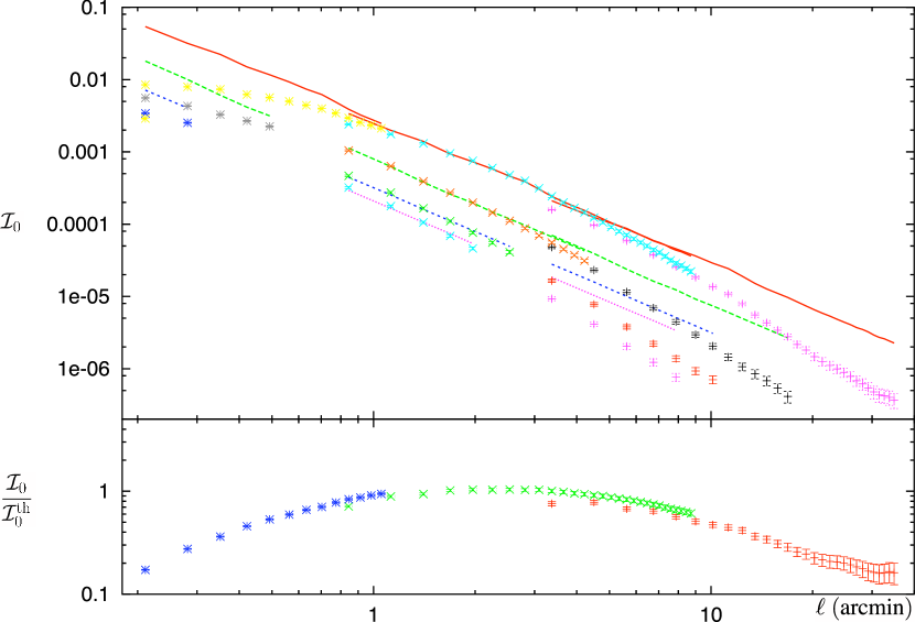
Figure 13: $\mathcal{I}_{0}$ measured in our three datasets. Results for all datasets are combined into this composite figure. In the top panel, top to bottom set of points corresponds to measurement for $\ell_{2}=r\ell_{3}$ for $r=1,2,3,4$. The corresponding theoretical prediction for $n=2$ are shown on top of the points for $r=1$ (solid line), $r=2$ (long dashed), $r=3$ (dashed) and $r=4$ (dotted). Bottom panel shows the ratio between the measurement and theoretical prediction for $r=1$.

Recall that our improved BvWM estimator uses the full ${\mathcal{F}}$ pseudo-vector. Using only the parity positive coordinate will further reduce the signal to noise by another factor $\sqrt{2}$ if its two components are uncorrelated.

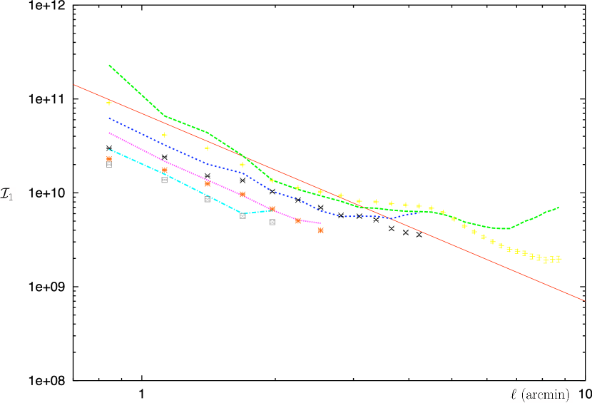
Figure 14: $\mathcal{I}_{1}$ measured in our medium resolution dataset. The solid line is a power law proportional to $1/\ell^{2}$ and shows the expected scaling. Other curves are semi analytical results (the covariance matrix has been evaluated from the simulations). They correspond to $r=1$ (long dashed), $r=2$ (dashed), 3 (dotted), $r=4$ (dot-dashed). Measurements partially agree with the semi-analytical predictions

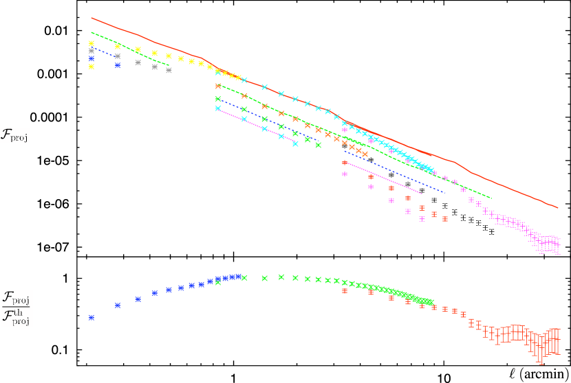
Figure 15: Same as Fig. 13 for our improved version of the BvWM estimator.

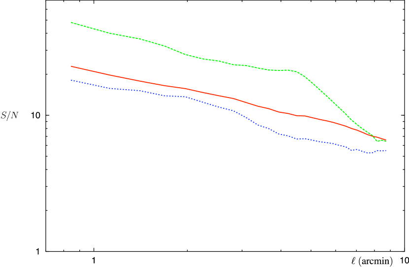
Figure 16: Signal to noise for $\mathcal{I}_{0}$ (solid line), $\mathcal{I}_{1}$ (dashed) and our improved version of the BvWM estimator (dotted). Only isoceles configurations have been taken into account. Data are projected on the $n=2$ model predictions. Only the medium resolution datasets are used.

6 Conclusion and Discussion

We have described a simplified analytic model that can be used to compute the three-point functions of the shear. This model is inspired by halo models, and only considers the one-halo contribution of a spherical potential of power law profile. The free parameters of our models are the profile index $n$ and a normalization. We have used this model to investigate some geometrical properties of the shear three-point function. In particular, we have shown that there is no preferred projection choice that will reduce the number of independent three-point functions.

We have compared the predictions of this model with results from N-body simulations. The predicted and measured three-point functions of the shear where shown to be in good agreement. In particular, we have shown that the approximation made on the profile index is sufficient to predict the shear three points function in a reasonable range of scales. The isothermal profile case, $n=2$, corresponding to scales from $1^{\prime}$ to $4^{\prime}$. These scales correspond indeed to the scales where the dominant halos at redshift $z=0.4$ are seen with a local profile index $n=2$. As expected, the smaller scales exhibited a behavior compatible with an index $n<2$, while larger scales where compatible with $n>2$. Our model allows for computations with a modified profile index, and it can thus be used at smaller or larger scales. However, at scales bigger than $4^{\prime}$, the one-halo dominant contribution model will break down, and one should take into account two and three halo terms Takada & Jain (2003b).

Using the agreement between our model and synthetic data, we proposed an optimized measurement of the cosmic shear three-point function. Our method trades the easier cosmological analysis allowed by $M_{ap}$ reconstructions methods for a better signal to noise of the measurement by avoiding cancellations. We use the model predictions to compute “optimal” weighted sums of the eight three-point functions. Contrarily to the $M_{ap}$ statistic, this kind of estimator is local and is not affected by the shape of the survey. These methods can be seen as a refined version of the one proposed by BvWM Bernardeau et al. (2003).

We computed two such estimators, the first a simple projection on our theoretical model, the other taking into account an estimation of the covariance matrix of the shear three-point functions. We compared them with an improved version of the estimator implemented by BvWM. Our estimators perform much better than the improved BvWM. The minimal variance estimator lets us expect more than a factor of two gain in the signal to noise in the best case.

With future space-based experiments, the quality of cosmic shear data will greatly increase and the loss of signal to noise inherent to compensated filters will be a not too high a price to pay for accessing to the filtered three-point function of the convergence. In the meantime, we believe that methods using projections of data onto theoretical predictions, as the one we proposed here, will be an interesting alternative. Improvement to what we proposed here will be doubtless needed. In our analysis, we first measured the three-point functions and then projected them on analytic templates, increasing the errors due to discreteness of the binning. We saw that this error has a significant impact on elongated isoceles configurations. Projecting the data as they are measured can solve this problem. Using a simple projection already improves the situation compared to what has been done before. The minimal variance estimator promises an even better ability to detect the shear three-point functions. Results from this estimator are yet difficult to forecast as our evaluation of the covariance matrix is somewhat noisy. More numerical simulations will be needed to quantify this better.

Improving the choice of effective halo profile index will also result in a net improvement, since by restricting the index to that of an isothermal sphere, $n=2$, we were only able to improve the efficiency of the three point function estimator around 1-4 arcminutes. This is not a restriction of the model, since it can be easily extended to any other index profile. More generally, given any model for the three-point functions one can compute the “optimal” estimators we define here.

Finally, we have not investigated how our method can be used to obtain information on the underlying cosmological model. With our simple model, all the cosmological information is encoded in the free normalization parameter. Further work, comparing our simple model, with a full halo model will be needed to investigate this point.

Appendix A Projection onto the opposite side

Here we describe the computations of the $\mathrm{trig}_{\mu}(2\phi_{i})$ factor for the opposite side projection described in section 3.1. Remember that the angles $\phi_{i}$ are defined by

$$\cos(\phi_{i})\equiv\frac{\left(\boldsymbol{u}-\boldsymbol{\theta}_{i}\right)\cdot\boldsymbol{\ell}_{i}}{\left|\boldsymbol{u}-\boldsymbol{\theta}_{i}\right|\ell_{i}}.$$

The computation of $\mathrm{trig}_{+}(2\phi_{i})=\cos(2\phi_{i})$ is the simplest. Defining $\boldsymbol{d}_{i}\equiv\boldsymbol{\theta_{i}}-\boldsymbol{u}$, one gets

$$\cos(\phi_{i})=\frac{\boldsymbol{\theta_{i}}\cdot\boldsymbol{\ell_{i}}-\frac{1}{2}\left(\theta_{i+1}^{2}-d_{i+1}^{2}-\theta_{i+2}^{2}+d_{i+2}^{2}\right)}{d_{i}\ell_{i}},$$

which, using the identity

$$2\boldsymbol{\theta_{i}}\cdot\boldsymbol{\ell_{i}}-\theta_{i+1}^{2}+\theta_{i+2}^{2}=\ell_{i+1}^{2}-\ell_{i+2}^{2}$$

reduces to

$$\cos(\phi_{i})=\frac{d_{i+1}^{2}-d_{i+2}^{2}+\ell_{i+1}^{2}-\ell_{i+2}^{2}}{2d_{i}\ell_{i}}.$$

The last step needed to obtain $\cos(2\phi_{i})$ is straightforward, using $\cos(2\phi_{i})=2\cos(\phi_{i})^{2}-1$, one gets the final expression of $\cos(2\phi_{i})$ as a polynomial of the 4th degree in $d_{i+1}$ and $d_{i+2}$ and second degree in $d_{i}$, divided by $d_{i}^{2}\ell_{i}^{2}$

$$\mathrm{trig}_{+}(2\phi_{1}) = \frac{1}{2d_{i}^{2}\ell_{i}^{2}}\left[d_{i+1}^{4}+d_{i+2}^{4}-2d_{i+1}^{2}d_{i+2}^{2}-2d_{i}^{2}\ell_{i}^{2}\right.$$

$$+2\left(d_{i+1}^{2}+d_{i+2}^{2}\right)\left(\ell_{i+1}^{2}-\ell_{i+2}^{2}\right)$$

$$\left.+\left(\ell_{i+1}^{2}-\ell_{i+2}^{2}\right)^{2}\right].$$

The parity negative terms require a little more work. One can use the identity $\sin(2\phi_{i})=2\cos(\phi_{i})\sin(\phi_{i})$. The difficulties lie in the computation of $\sin(\phi_{i})$. One can use the fact that

$$\sin(\phi_{i})=\frac{\left(\boldsymbol{u}-\boldsymbol{\theta}_{i}\right)\wedge\boldsymbol{\ell}_{i}}{\left|\boldsymbol{u}-\boldsymbol{\theta}_{i}\right|\ell_{i}}\cdot\boldsymbol{z},$$ (46)

and re-express the unit vector $\boldsymbol{z}$ as

$$\boldsymbol{z}=\frac{\boldsymbol{\ell}_{i+2}\wedge\boldsymbol{\ell}_{i}}{\ell_{i+2}\ell_{i}\sin(\psi_{i+1})}.$$ (47)

Finally, a careful invocation of the identity

$$\left(\boldsymbol{A}\wedge\boldsymbol{B}\right)\cdot\left(\boldsymbol{C}\wedge\boldsymbol{D}\right)+\left(\boldsymbol{B}\cdot\boldsymbol{B}\right)\left(\boldsymbol{C}\cdot\boldsymbol{D}\right) =$$

$$\left(\boldsymbol{A}\wedge\boldsymbol{C}\right)\cdot\left(\boldsymbol{B}\wedge\boldsymbol{D}\right)+\left(\boldsymbol{A}\cdot\boldsymbol{C}\right)\left(\boldsymbol{B}\cdot\boldsymbol{D}\right)$$

allows us to re-express Eq. (46) as

$$\sin(\phi_{i}) = \frac{1}{d_{i}\ell_{i}^{2}\ell_{i+2}\sin(\psi_{i+1})}\left\{-\left(\boldsymbol{u}-\boldsymbol{\theta}_{i}\right)\cdot\boldsymbol{\ell}_{i}\,\boldsymbol{\ell}_{i}\cdot\boldsymbol{\ell}_{i+2}\right.$$ (49)

$$\hskip 8.5359pt\left.+\left[\left(\boldsymbol{u}-\boldsymbol{\theta}_{i+2}\right)+\left(\boldsymbol{\theta}_{i+2}-\boldsymbol{\theta}_{i}\right)\right]\cdot\boldsymbol{\ell}_{i+2}\,\ell_{i}^{2}\right\}$$

which can be written as a function of $\cos(\phi_{i+2})$ and $\cos(\phi_{i})$ and a term that only depends on the configuration

$$\sin(\phi_{i}) = \frac{1}{d_{i}\ell_{i}^{2}\ell_{i+2}\sin(\psi_{i+1})}\left(\cos(\phi_{i+2})d_{i+2}\ell_{i+2}\,\ell_{i}^{2}\right.$$ (50)

$$\hskip 8.5359pt\left.+\cos(\phi_{i})d_{i}\ell_{i}\,\boldsymbol{\ell}_{i}\cdot\boldsymbol{\ell}_{i+2}+\boldsymbol{\ell}_{i+1}\cdot\boldsymbol{\ell}_{i+2}\ell_{i}^{2}\right).$$

This last expression can be expressed only in terms of $\ell_{j=1,2,3}$ and $d_{j=1,2,3}$ as the ratio between a 4th degree polynomial in the $d_{j=1,2,3}$ divided by $d_{i}$, the coefficient being functions of the $\ell_{j=1,2,3}$. After simplifications, the final result for $\mathrm{trig}_{\times}(2\phi_{i})=\sin(2\phi_{i})$reads

$$\mathrm{trig}_{\times}(2\phi_{i}) = \frac{\left(d_{i+1}^{2}-d_{i+2}^{2}+\ell_{i+1}^{2}-\ell_{i+2}^{2}\right)}{2d_{i}^{2}\ell_{i}^{2}\sqrt{4\ell_{i+1}^{2}\ell_{i+2}^{2}-\left(\ell_{i}^{2}-\ell_{i+1}^{2}-\ell_{i+2}^{2}\right)^{2}}}$$ (51)

$$\times\left[-2d_{i}^{2}\ell_{i}^{2}+d_{i+1}^{2}\left(\ell_{i}^{2}+\ell_{i+1}^{2}-\ell_{i+2}^{2}\right)\right.$$

$$+d_{i+2}^{2}\left(\ell_{i}^{2}-\ell_{i+1}^{2}+\ell_{i+2}^{2}\right)+\ell_{i+1}^{4}+\ell_{i+2}^{4}$$

$$\left.-\ell_{i}^{2}\left(\ell_{i+1}^{2}+\ell_{i+2}^{2}\right)+2\ell_{i+1}^{2}\ell_{i+2}^{2}\right]$$

Appendix B Numerical simulations

We used the GADGET Springel et al. (2001) code to evolve 24 realizations of the large scale structure in a small section of a FRLW universe with parameters $\Omega_{m}=0.3$, $\Omega_{\Lambda}=0.7$ $h=0.7$. The initial conditions were imposed at redshift $z=50$ using second-order Lagrangian perturbation theory Scoccimarro (1998). The initial power spectrum used was obtained using the B&E Bond & Efstathiou (1984) fitting formula and normalized to $\sigma_{8}=0.9$ at $z=0$ in linear theory. The boxes we considered are cubes of $(100\,\textrm{Mpc}/h)^{3}$ containing $200^{3}$ particles. This choice has been made has a trade-off between speed and accuracy. The simulation were run on $24$ nodes of our cluster. For each realization, we took a snapshot of the large scale structures every $100$ Mpc/$h$.

B.1 Building the light-cone

We use these snapshots to compute the weak lensing effect at a redshift of unity on a square light cone. At $z=1$ the sides of the boxes represent $2.47$ degrees. We will only produce $2.4^{2}$ square-degrees patches of the sky.

The line of sight to the sources, is built by tilling $17$ snapshots at different redshifts. We use this construction to create more pseudo realizations of the lensing effect that we have different realizations of the density field. We follow a very similar method to the one exposed by White and Hu in White & Hu (2000).

While building each line of sight, we will make sure that each N-body realization is only used once. To increase the randomness of our lensing pseudo-realization, we translate each snapshot by a random vector, taking advantage of the periodic boundary condition of the boxes. Moreover, we trace the path of the photon along a random direction in the box, and not along the axis direction. Note however that all rotation angles are not allowed if one wants to avoid tracing twice the same structures in a given box. We take this problem into account when picking the ray-tracing direction.

The projected mass density is then built as follows. For each of our $17$ snapshots, after translation and rotation, we build a list of particles belonging to the light cone. This list of particles is flattened onto a 2D density map, using a Cloud-in-Cell algorithm. This 2D map is then multiplied by the efficiency window function of the lensing effect to provide a map of the convergence $\kappa$. These $\kappa$ slices are added to produce the final lens effect on the source plane. The shear field $\boldsymbol{\gamma}$ on each of these synthetic $\kappa$ maps is obtained by numerically solving Eq. (3) with a FFT Van Waerbeke et al. (2001).

Note that in our computation of the lens effect we neglected some secondary effects. For example our ray-tracing scheme is strictly restricted to the Born approximation. We thus assume here that the lens effect computed along the unperturbed path of the photon gives a good evaluation of the effect. This as been tested in numerous work before Van Waerbeke et al. (2001); Jain et al. (2000). Doing this, we neglect the lens lens-coupling which is known to produce non-zero corrections to the three-point function of the convergence field. This correction is expected to be small Van Waerbeke et al. (2001), and we will neglect it here as our goal is mainly to evaluate the validity of our simplified halo model.

The number of slices of our light-cone is more of a concern. A naive evaluation of the impact of this choice can be made by comparing a step summation of the filtered lensing power spectrum with its full integration. For an Einstein-deSitter universe, assuming a power law matter density fluctuation, we thus have to compare step summation and integration of the function

$$R(t)=x^{4-n}(x-1)^{2}.$$ (52)

For the spectral index $n\sim-\frac{3}{2}$, the difference between the summation and integration falls below one percent as soon as the number of slices is bigger than 5. Vale and White Vale & White (2004) recently performed a less naive evaluation of the same effect using N-body simulations. They showed that with simulations comparable to ours ($300$Mpc and $512^{3}$particles) one can expect about 5% discrepancy on the power spectrum between a computation with a slice every $\Delta s=125$Mpc (we are slicing every $100$Mpc ) and one with $\Delta s=25$Mpc.

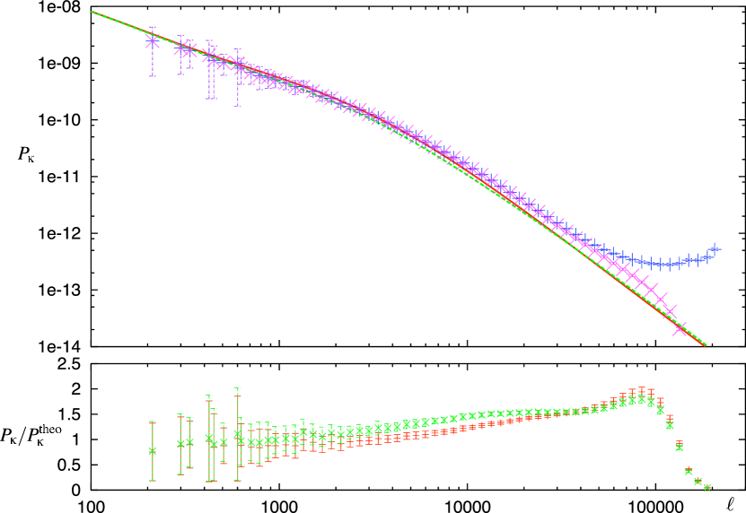
Figure 17: Power spectrum of $\kappa$ measured on the 40 lensing pseudo-realization. Lines are the predicted power spectrum using the PD Peacock & Dodds (1996) (dashed) or halofit Smith et al. (2003) (solid) prescription for the small scales. Points are the measurements in the simulations, without smoothing (crosses), and with smoothing (xs) to remove the Poisson noise (see text). Bottom panel shows the ratio between the smoothed measured power spectrum and the two predictions using PD (xs) and halofit (crosses).

B.2 Resolution

During the Cloud-in-Cell remapping of the particle list, the interpolation was done on a $2048^{2}$ grid. The maximum resolution of our simulation is thus $4.21$ arc-sec. However, at this scale we expect to probe the region where shot noise starts to dominate [see equation (24) from Jain et al. (2000)]. To reduce shot noise contributions we smooth the $\kappa$ maps by a 2 pixel wide Gaussian window.

The average over our 40 realizations of the $\kappa$ power spectrum is presented Fig. 17 and compared with the theoretical one obtained by two ansatz of the non-linear density power spectrum. The power spectrum is somewhat higher than the analytical predictions in the non-linear regime. A similar behavior can be seen in the 3D power spectrum of our simulations.

B.3 Measurement strategy

The measurement of two and three point functions in real space requires significant computing time. These operations scale respectively as $N^{2}$ and $N^{3}$ where $N=2048^{2}$ in our case. To reduce the time needed to perform the computation, we will only probe configurations up to a cut-off scale. This reduces the amount of computer time needed to perform the measurement, but prevents us to access to a broad range of scales.

To reduce the computation cost yet preserving the ability to measure the three-point functions over a large range of scales, we measure the two- and three-point functions at large scales on degraded resolution maps obtained by top-hat filtering and regridding the synthetic shear fields. For each field, we produced three datasets; one with the nominal resolution of $2048^{2}$ pixels representing of $4.22^{2}$ arc-sec², one with a four time degraded resolution ($512^{2}$ pixels, $16.9^{2}$ arc-sec²) and the last with a sixteen time degraded resolution ($128^{2}$ pixels, $1.125^{2}$ arc-min²). For the two-point functions, the computation cost is lower and we are able, for the two last resolution sets to measure it without cut-off scale; we apply a cut-off only for the biggest map and only consider scales smaller than a 32th of the map size.

For the three-point functions we only explore a small region of the three points configuration space. Table 1 presents the scales probed by each of our datasets.

	max	medium	min
$\Delta\ell$	$4.22^{\prime\prime}$	$16.9^{\prime\prime}$	$1.125^{\prime}$
$\ell_{\textrm{max}}$	$67.5^{\prime\prime}$	$9.0^{\prime}$	$36^{\prime}$

Table 1: Description of the three datasets. Max is the best resolution dataset, min the worst one. Thorough this article, we will mainly use the medium resolution.

The cut-off scales have been chosen so as to have each measurement to require about ten days of computation time of one node of the our cluster.

We take into account the cut-off scale we added to optimize the measurement. Since the data are gridded, we can precompute for any given point all the positions of the couples of points which will create a valid configuration. By valid configuration we mean any triangle that fits the requirement of the cut-off scale, whose three point function measured with a given projection convention has a meaningful result (i.e. for the center of mass projection, we throw out configurations where the center of mass is one of the vertices of the triangle) and is such that a given configuration is only seen once when varying the initial position. This last requirement can be fulfilled by requiring that for any couple of points

$$x_{1}\geq x_{i},\,x_{2}\geq x_{1}\,y_{1}>y_{i} x_{1}=x_{i},$$ if

$$y>y_{1} x_{2}=x_{1},$$ if (53)

provided that the initial point will go through the grid increasing its $y_{i}$ position first.

We build a table containing for each of such configuration, the offset of the points positions, as well as the projector vectors on the $+$ and $\times$ direction for each point of the triangle. Populating this table is an expensive task as it goes as $l^{4}$ in time and memory, where $l$ is our cut-off scale. Once this initialization done, however, we just have to traverse the shear map and apply for each point the rules contained in the initialization table.

B.4 Shear two-point functions

We measured the two point functions of the shear $\xi_{\pm}$

$$\xi_{\pm}(\theta)=\left\langle\gamma_{+}\gamma_{+}(\theta)\right\rangle\pm\left\langle\gamma_{\times}\gamma_{\times}(\theta)\right\rangle,$$ (54)

where the shear pseudo-vector is projected to the $+$ and $\times$ directions defined by the vector linking the two points and the same vector rotated by $\pi/4$ (see section 2.2). The relation between the shear two-point functions and the power spectrum of the convergence is well known Kaiser (1992)

$$\xi_{\pm}(\theta)=\int\mathrm{d}l\,l\,P_{\kappa}(l)\,J_{0,4}(l\theta).$$ (55)

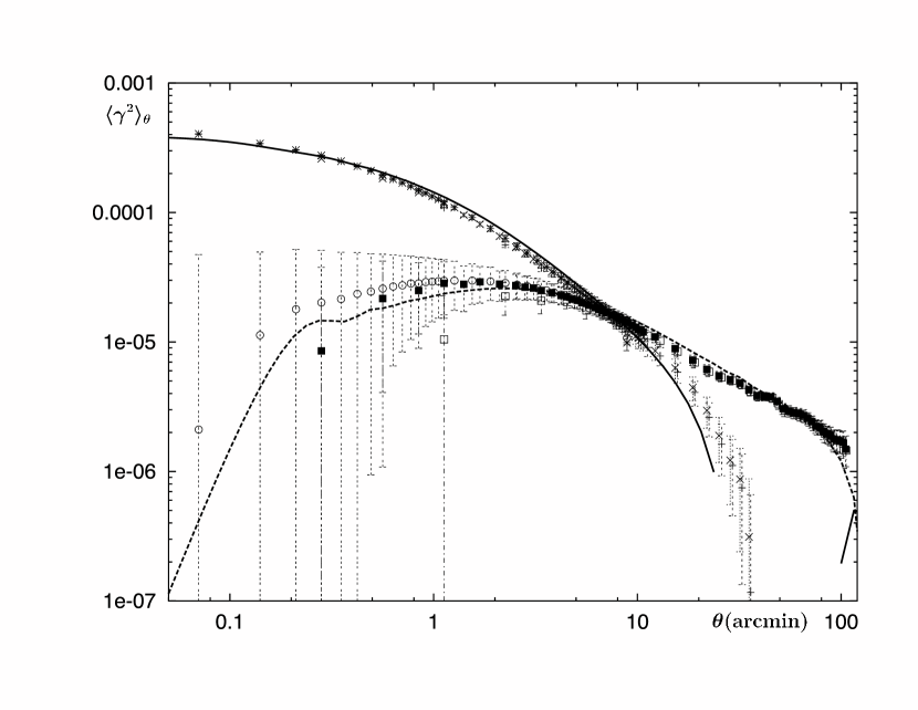
Figure 18: The shear two-point functions in the simulations. Lines are the predicted power spectrum, taking into account the survey size and resolution. Solid line is $\xi_{+}$, dashed, $\xi_{-}$. Points show the measurements in the 40 realizations, for our three different datasets. The open circle (resp. plain squares, open squares) shows $\xi_{-}$ and regular pluses (resp crosses,dashed pluses) $\xi_{+}$, measured in the max (resp medium, min) resolution datasets.

Figure 18 presents the measurement of $\xi_{\pm}$ in our simulations as well as analytical predictions. It can be surprising to see that at a scale corresponding to only a fourth of the box scale, the two point shear correlations, and especially the $\xi_{+}$ one, differ greatly from the usual analytical prediction. This corresponds to the effect of the finite survey size. Even at a scale four times smaller than our survey size, we are already suffering from the lack of large-scale correlations. We can reproduce it in our analytical prediction as follows: we are filtering the convergence power spectrum by a Bessel $J_{0}$ or $J_{4}$ function. $J_{0}$ and $J_{4}$ are maximum when their argument is small. This means that when the angular scale is large, the filter overweights the small $l$ in $P(l)$. This is more severe for $J_{0}$ as its envelope decrease more quickly than the one of $J_{4}$. Even though $l\,P(l)$ quickly decrease when $l$ goes to $0$, it amounts to a difference that can be observed in the comparison between analytical computations and measurements. If we artificially cut the analytical power spectrum in our computation to reproduce the absence of scale larger than $\sqrt{2}\times 2.4$ arc-minutes in our simulation, we obtain a far better agreement with our measurement.

Similarly, the small scale behavior of $\xi_{\pm}$ is modified by the filtering we applied to our synthetic field by downgrading their resolution. The analytic predictions, once this filtering is included, are in good agreement with our numerical results.

We are thus quite confident than our implementation of the measurement is sound and that the resolution degradation procedure gives meaningful results.

References

- Bartelmann & Schneider (2001) Bartelmann, M. & Schneider, P. 2001, Phys. Rep, 340, 291
- Benabed & Bernardeau (2001) Benabed, K. & Bernardeau, F. 2001, Phys. Rev. D, 64, 83501
- Benabed & Van Waerbeke (2004) Benabed, K. & Van Waerbeke, L. 2004, Phys. Rev. D, 70, 123515
- Bernardeau et al. (2002) Bernardeau, F., Mellier, Y., & van Waerbeke, L. 2002, A&A, 389, L28
- Bernardeau et al. (1997) Bernardeau, F., van Waerbeke, L., & Mellier, Y. 1997, A&A, 322, 1
- Bernardeau et al. (2003) Bernardeau, F., van Waerbeke, L., & Mellier, Y. 2003, A&A, 397, 405
- Bond & Efstathiou (1984) Bond, J. R. & Efstathiou, G. 1984, ApJ, 285, L45
- Brown et al. (2002) Brown, M. L., Taylor, A. N., Hambly, N. C., & Dye, S. 2002, MNRAS, 333, 501
- Catelan et al. (2001) Catelan, P., Kamionkowski, M., & Blandford, R. D. 2001, MNRAS, 320, L7
- Cooray & Hu (2002) Cooray, A. & Hu, W. 2002, ApJ, 574, 19
- Cooray & Sheth (2002) Cooray, A. & Sheth, R. 2002, Phys. Rep, 372, 1
- Crittenden et al. (2001) Crittenden, R. G., Natarajan, P., Pen, U., & Theuns, T. 2001, ApJ, 559, 552
- Crittenden et al. (2002) Crittenden, R. G., Natarajan, P., Pen, U., & Theuns, T. 2002, ApJ, 568, 20
- Heymans & Heavens (2003) Heymans, C. & Heavens, A. 2003, MNRAS, 339, 711
- Hoekstra (2004) Hoekstra, H. 2004, MNRAS, 347, 1337
- Jain et al. (2000) Jain, B., Seljak, U. ., & White, S. 2000, ApJ, 530, 547
- Jarvis et al. (2004) Jarvis, M., Bernstein, G., & Jain, B. 2004, MNRAS, 352, 338
- Jarvis & Jain (2004) Jarvis, M. & Jain, B. 2004, astro-ph/0412234
- Jarvis et al. (2005) Jarvis, M., Jain, B., Bernstein, G., & Dolney, D. 2005, astro-ph/0502243
- Kaiser (1992) Kaiser, N. 1992, ApJ, 388, 272
- King & Schneider (2002) King, L. & Schneider, P. 2002, A&A, 396, 411
- Navarro et al. (1997) Navarro, J. F., Frenk, C. S., & White, S. D. M. 1997, ApJ, 490, 493
- Peacock & Dodds (1996) Peacock, J. A. & Dodds, S. J. 1996, MNRAS, 280, L19
- Pen et al. (2003) Pen, U., Zhang, T., van Waerbeke, L., et al. 2003, ApJ, 592, 664
- Refregier (2003) Refregier, A. 2003, ARA&A, 41, 645
- Schneider (2003) Schneider, P. 2003, A&A, 408, 829
- Schneider et al. (2005) Schneider, P., Kilbinger, M., & Lombardi, M. 2005, A&A, 431, 9
- Schneider & Lombardi (2003) Schneider, P. & Lombardi, M. 2003, A&A, 397, 809
- Schneider et al. (2002) Schneider, P., van Waerbeke, L., Kilbinger, M., & Mellier, Y. 2002, A&A, 396, 1
- Scoccimarro (1998) Scoccimarro, R. 1998, MNRAS, 299, 1097
- Smith et al. (2003) Smith, R. E., Peacock, J. A., Jenkins, A., et al. 2003, MNRAS, 341, 1311
- Springel et al. (2001) Springel, V., Yoshida, N., & White, S. D. M. 2001, New Astronomy, 6, 79
- Takada & Jain (2002) Takada, M. & Jain, B. 2002, MNRAS, 337, 875
- Takada & Jain (2003a) Takada, M. & Jain, B. 2003a, ApJ, 583, L49
- Takada & Jain (2003b) Takada, M. & Jain, B. 2003b, MNRAS, 340, 580
- Takada & Jain (2003c) Takada, M. & Jain, B. 2003c, MNRAS, 344, 857
- Vale & White (2004) Vale, C. & White, M. 2004, Astroparticle Physics, 22, 19
- Van Waerbeke et al. (2001) Van Waerbeke, L., Hamana, T., Scoccimarro, R., Colombi, S., & Bernardeau, F. 2001, MNRAS, 322, 918
- White & Hu (2000) White, M. & Hu, W. 2000, ApJ, 537, 1
- Zaldarriaga & Scoccimarro (2003) Zaldarriaga, M. & Scoccimarro, R. 2003, ApJ, 584, 559