The lithium content of the Galactic Halo stars

Thanks to the accurate determination of the baryon density of the universe by the recent cosmic microwave background experiments, updated predictions of the standard model of Big Bang nucleosynthesis now yield the initial abundance of the primordial light elements with unprecedented precision. In the case of ⁷Li, the CMB+SBBN value is significantly higher than the generally reported abundances for Pop II stars along the so-called Spite plateau. In view of the crucial importance of this disagreement, which has cosmological, galactic and stellar implications, we decided to tackle the most critical issues of the problem by revisiting a large sample of literature Li data in halo stars that we assembled following some strict selection criteria on the quality of the original analyses.

In the first part of the paper we focus on the systematic uncertainties affecting the determination of the Li abundances, one of our main goal being to look for the “highest observational accuracy achievable” for one of the largest sets of Li abundances ever assembled. We explore in great detail the temperature scale issue with a special emphasis on reddening. We derive four sets of effective temperatures by applying the same colour-${\rm T}_{\rm eff}$  calibration but making four different assumptions about reddening and determine the LTE lithium values for each of them. We compute the NLTE corrections and apply them to the LTE lithium abundances. We then focus on our “best” (i.e. most consistent) set of temperatures in order to discuss the inferred mean Li value and dispersion in several ${\rm T}_{\rm eff}$ and metallicity intervals. The resulting mean Li values along the plateau for [Fe/H] $\leq$ -1.5 are $A(Li)_{NLTE}$ = 2.214$\pm$0.093 and 2.224$\pm$0.075 when the lowest effective temperature considered is taken equal to 5700 K and 6000 K respectively. This is a factor of $\sim$ 2.48 to 2.81 (depending on the adopted SBBN model and on the effective temperature range chosen to delimit the plateau) lower than the CMB+SBBN determination. We find no evidence of intrinsic dispersion. Assuming the correctness of the CMB+SBBN prediction, we are then left with the conclusion that the Li abundance along the plateau is not the pristine one, but that halo stars have undergone surface depletion during their evolution.

In the second part of the paper we further dissect our sample in search of new constraints on Li depletion in halo stars. By means of the Hipparcos parallaxes, we derive the evolutionary status of each of our sample stars, and re-discuss our derived Li abundances. A very surprising result emerges for the first time from this examination. Namely, the mean Li value as well as the dispersion appear to be lower (although fully compatible within the errors) for the dwarfs than for the turnoff and subgiant stars. For our most homogeneous dwarfs-only sample with [Fe/H]$\leq$-1.5, the mean Li abundances are $A(Li)_{NLTE}$ = 2.177$\pm$0.071 and 2.215$\pm$0.074 when the lowest effective temperature considered is taken equal to 5700 K and 6000 K respectively. This is a factor of 2.52 to 3.06 (depending on the selected range in ${\rm T}_{\rm eff}$ for the plateau and on the SBBN predictions we compare to) lower than the CMB+SBBN primordial value. Instead, for the post-main sequence stars the corresponding values are 2.260$\pm$0.1 and 2.235$\pm$0.077, which correspond to a depletion factor of 2.28 to 2.52.

These results, together with the finding that all the stars with Li abnormalities (strong deficiency or high content) lie on or originate from the hot side of the plateau, lead us to suggest that the most massive of the halo stars have had a slightly different Li history than their less massive contemporaries. In turn, this puts strong new constraints on the possible depletion mechanisms and reinforces Li as a stellar tomographer.

1 The Lithium Paradigm

From the time of its discovery in the stellar atmospheres of very metal-poor Population II stars (Spite & Spite 1982a), lithium has been considered a key diagnostic to test and constrain our understanding and description of the primordial Universe, of stellar interiors and evolution, and of spallation physics (for the latter two especially so if combined with abundances of beryllium and boron).

Lithium-7 is one of the four primordial isotopes that have been formed in observable quantities by nuclear reactions during the first minutes of the Universe (e.g. Olive, Steigman, & Walker 2000 and references therein). Together with deuterium, helium-3 and helium-4, knowledge of its primordial abundance provides one of the main observational constraints on the baryon-to-photon ratio $\eta\propto\Omega_{b}h^{2}$ which is the only free parameter of the standard Big Bang Nucleosynthesis (SBBN).

Among these light elements, lithium is one of the easiest to observe (its resonant doublet falls at 670 nm, i.e. easily accessible from ground telescopes even of small sizes), which explains the wealth of data available in the literature.

Another reason for such a large literature database is connected to the important finding of a remarkably flat and constant Li abundance among Galactic halo dwarf stars spanning a wide range of effective temperatures and metallicities (the so-called Spite plateau, cf Spite & Spite 1982a,b). This result came as a surprise. At that time indeed it was generally believed that the primordial A(Li) abundance was in the range 3.0–3.3, which corresponds to the value measured in meteorites and also to the maximum value detected in Population I stars, both in the field and in open clusters (see the review by Boesgaard & Steigman 1985). If this were the case, then the “constant” but lower value of lithium along the Spite plateau would have required that all the oldest stars of our Galaxy had suffered a uniform depletion by about a factor of 10. Although several mechanisms could be conjectured to modify the surface lithium abundance (proto-stellar destruction, microscopic diffusion, turbulent diffusion, mass loss), they were also suspected to depend on the stellar mass (i.e., on the effective temperature). Consequently the constancy of the Li plateau was used (and is actually still used very often) as an argument to say that these processes were in fact not efficient in Pop II stars.

The other interpretation was then that the plateau value represents the amount of Li produced during the Big Bang, and that the Galaxy had been enriched in its Li content by a factor of at least 10 since its birth. The fact that lithium is produced in several other nucleosynthetic sites (i.e. $\alpha-\alpha$ fusion, spallation reactions, late stellar evolutionary stages, like AGB stars, novae, etc.; see Romano et al. 2003 and references therein), none of which has been quantitatively and accurately estimated nor strongly constrained by observations, complicates the final interpretation of its Galactic evolution.

Recent results on cosmic microwave background anisotropies, most particularly from the Wilkinson Microwave Anisotropy Probe (WMAP) experiment (Bennet et al. 2003; Spergel et al. 2003) allowed an unprecedented precision on the determination of the baryon-to-photon ratio $\eta$ and revealed that Li seems to lie between the two extreme solutions discussed above. The WMAP data alone lead to $\Omega_{b}h^{2}=0.0237\pm 0.001$, or $\eta=6.5^{+0.4}_{-0.3}\times 10^{-10}$. When combined with additional CMB experiments (CBI, Pearson et al. 2003; ACBAR, Kuo et al. 2002) and with measurements of the power spectrum (2dF Galaxy Redshift Survey, Percival et al. 2001; Ly$\alpha$ forest, Croft et al. 2002, Gnedin & Hamilton 2002), the resulting values are $\Omega_{b}h^{2}=0.0224\pm 0.0009$ or $\eta=6.1^{+0.3}_{-0.2}\times 10^{-10}$. With this value of $\eta$, updated SBBN predictions now allow a precise determination of the primordial abundances of the light elements D, ³He, ⁴He and ⁷Li that we can compare with observations in low-metallicity environments. The WMAP+SBBN determinations of these abundances in the most two recent studies (Coc et al. 2004, Cyburt 2004, Serpico et al. 2004) are summarised in Table 1.

Table 1: WMAP+SBBN primordial abundances predicted when $\eta=(6.14\pm 0.25)\times 10^{-10}$ (or $\Omega_{b}h^{2}=0.0224\pm$0.0009; Spergel et al. 2003) is adopted

	Coc et al. (2004)	Cyburt (2004)	Serpico et al. (2004)
D/H	(2.60${}^{+0.19}_{-0.17})\times 10^{-5}$	(2.55${}^{+0.21}_{-0.20})\times 10^{-5}$	(2.58${}^{+0.19}_{-0.16})\times 10^{-5}$
YP	0.2479$\pm$0.0004	0.2485$\pm$0.0005	0.2479$\pm$0.0004
3He/H	(1.04$\pm 0.04)\times 10^{-5}$	(1.01$\pm 0.07)\times 10^{-5}$	1.03$\pm$0.03
. 7Li/H	(4.15${}^{+0.49}_{-0.45})\times 10^{-10}$	(4.26${}^{+0.91}_{-0.86}\times)10^{-10}$	(4.6${}^{+0.4}_{-0.4})\times 10^{-10}$

A very good agreement is achieved between the primordial abundance of deuterium derived from WMAP+SBBN and the average value of D/H observations in cosmological clouds along the line of sight of quasars (Kirkman et al. 2003). On the other hand the observational data of ³He in galactic HII regions are scarce and must be corrected for contamination of the observed gas by ejecta from earlier generations of stars (e.g. Tosi 1998, Charbonnel 2002). The upper limit to the primordial abundance recommended by Bania et al. (2002) is however quite consistent with the CMB-derived value. Finally the CMB-predicted primordial ⁴He abundance is higher than the values derived from the determinations in complex low-metallicity HII regions (both galactic and extra-galactic) and the extrapolation to zero oxygen abundance (Izotov & Thuan 2004, Olive & Skillman 2004 and references therein). However the difference is relatively modest (2-3$\%$) and it may simply call for further exploration of the systematic effects in the abundance analysis.

The most critical case concerns ⁷Li, the CMB-derived primordial abundance of which is clearly higher (by about a factor of 3) than the current determinations in low-metallicity halo stars. This result seems to be very robust with respect to the nuclear uncertainties on the SBBN reactions although Coc et al. (2004) show that the discrepancy could be resolved by an increase of a factor of $\sim$ 100 of the ⁷Be(d,p)2⁴He reaction rate. Although this is not supported by the data currently available, this issue has to be further investigated experimentally. Should this nuclear solution be excluded, we would then be left with the astrophysical solution. Namely, with the conclusion that the Li abundance that we see at the surface of halo stars is not the pristine one, but that these stars have undergone surface lithium depletion at some point during their evolution. This possibility has been discussed many times in the literature. Several physical mechanisms have been invoked, but all the current models encounter considerable difficulties to reconcile a non negligible depletion of lithium with both the flatness and the small dispersion along the so-called Li plateau (see the review by Pinsonneault et al. 2000 and Talon & Charbonnel 2004 for more recent references). The challenge thus still remains to identify the process (or processes) by which a reduction by a factor of $\sim$3 could occur so uniformly in stars over a large range in effective temperature and metallicity.

With the CMB constraint, we are now entering a golden age for Li as both a baryometer and a stellar tomographer. In this quest however one has still to pay special attention to the observational analysis and determination of the lithium abundances in the most metal-poor, thus the oldest stars of our Galaxy. As a matter of fact and despite the large number of spectroscopic data that has become available in the last two decades, there are still on-going debates on the patterns of the plateau, like its thinness, the possible existence of a spread and of a dependence of A(Li) with metallicity and effective temperature. These characteristics must be precisely determined in order to constrain the physical processes which lead to Li depletion in Pop II stars as well as those of Galactic production.

2 The “Lithium Plateau Debate”?

Deliyannis et al. (1993) were among the first to present evidence for the existence of dispersion (of the order of $\pm$20% about the mean, derived from the “equivalent width-colour” plane), followed by Thorburn (1994) and Norris et al. (1994), the latter being the first to also have found a dependence of A(Li) on both ${\rm T}_{\rm eff}$   and metallicity. Molaro et al. (1995) counter-argued these findings showing that when a fully consistently determined temperature scale is used (in their case, the Fuhrmann et al. 1994 scale, derived from Balmer lines fitting), no dispersion nor tilt is found (Li abundances are mostly sensitive to ${\rm T}_{\rm eff}$ ), but they were shortly followed by Ryan et al. (1996) who once again confirmed the slopes. They argued that the Molaro et al. sample was plagued by the inclusion of subgiants that may have affected their final outcome. On the intrinsic scatter issue, they noted that there were some stars, characterized by very similar parameters (colour, ${\rm T}_{\rm eff}$  and metallicity), but that turned out from multiple measurements to have very different Li abundances. The debate kept being very alive: Spite et al. (1996) explored further the ${\rm T}_{\rm eff}$  scale issue (comparing different ${\rm T}_{\rm eff}$  determinations) and found that the rms scatter of the Li abundance was between 0.06 and 0.08 dex, hence very small if real. Bonifacio & Molaro (1997) re-selected their sample, this time excluding possible outliers (like the abovementioned subgiants) and once again came to the conclusion of no intrinsic dispersion nor dependence of A(Li) on metallicity, but of a tiny trend with the temperature. They concluded that the finding or not of a trend with effective temperature may well depend on the adopted ${\rm T}_{\rm eff}$  scale.

It is only towards the end of the 90s when a full agreement on the absence of intrinsic dispersion was reached: Ryan et al. (1999), by analysing a new sample of 23 stars covering a narrow range in ${\rm T}_{\rm eff}$  (6050-6350 K) and in metallicity ($-$3.5 – $-$2.5), claimed that the intrinsic spread is effectively zero, i.e. 0.031 dex, at the 1$\sigma$ level (to be compared to their formal errors of 0.033 dex). However, they still recovered the dependence on metallicity, at the level of dA(Li)/d[Fe/H] = 0.118$\pm$0.023 (1$\sigma$) dex per dex, i.e. very similar to the slopes previously found. The trend with ${\rm T}_{\rm eff}$  , if any, is likely to be meaningless because of the very narrow ${\rm T}_{\rm eff}$   range there explored.

This is when we started developing our project. By comparing the data samples analysed by different authors (starting with the Bonifacio & Molaro 1997 and Ryan et al. 1996, 1999 because of their final, opposite claims) we noticed that for some stars, common to several analyses, very discrepant Li abundances were reported, which could have clearly influenced some of the early claims for dispersion, and they could still play a role in the current debate about the existence of a slope between Li and ${\rm T}_{\rm eff}$   and [Fe/H].

In order to further tackle these issues, we decided to re-analyse the large sample of Li abundances available in the literature (§ 3 and 4) from a different perspective. One of our main goals is to focus on the systematic uncertainties affecting the determination of Li abundances. First, because the Li abundance is strongly dependent on the assumed temperature, we explore further the temperature scale issue (§ 5) with the aim of deriving what the best achievable accuracy may be for a temperature scale derived in a consistent manner. We put special emphasis on reddening, usually an underestimated source of error. We derive four sets of effective temperatures by applying the same colour-T_eff calibration but making four different assumptions about reddening. We then derive the LTE lithium abundances for each of these sets and compute the NLTE corrections. Then we select our “best” (in terms of consistency) set of temperatures in order to determine the mean Li abundance and the dispersion for one of the largest sample of halo stars ever studied in a consistent way (§ 6 and 7). This allows us to derive preliminary results on the mean lithium abundance and dispersion which can be compared to previous analyses (§ 8).

Secondly we look afresh at our Li abundances together with the evolutionary status of each target (§ 9) in order to get clues on the internal processes that may have been involved in modifying the Li abundances along the Plateau. This is why we did not restrict a priori our sample to any specific evolutionary status. We then discuss the lithium abundance along the plateau for the dwarf stars only (§ 10) and look at its behaviour in subgiants (§ 11). We test whether our results on the dispersion and trends can be altered by the presence of binary stars in the sample (§ 12), and we finally inspect the cases of stars with extreme lithium abundances (§ 13). Then we discuss the current status of Pop II stellar models in view of our observational results (§ 14). Finally we summarise our results and conclude on some remaining open questions (§ 15).

3 Sample selection: A Critical analysis of the literature

The database of Li abundances measured in Galactic stars and available in the literature is huge. During this work, we restricted our search to the main observational analyses from the early 90 onwards.

Table 2: Literature sources

Authors	R	S/N	T/g/Fea	Noteb
1. Ryan et al. 1996	38,000	$>$100	p/l/l	O,T
2. Ryan et al. 1999	40,000	$>$100	p/l/l	T
3. Ryan et al. 2001a,b	50,000	$>$100	p/l/l	O,T
4. Bonifacio & Molaro 1997	…	…	p/l/l	T
5. Pilachowski et al. 1993	30,000	$>$100	p/p/s	O
6. Hobbs & Thorburn 1991	30,000	$>$100	l/l/l	O,T
7. Thorburn 1994	28,000	$>$80	p/l/l	O
8. Molaro et al. 1995	…	…	p/l/l	T
9. Spite et al. 1996	…	$>$80	p/p/s	T
10. Ryan & Deliyannis 1998	42,000	$>$70	p/p/s	O
11. Gutierrez et al. 1999	30,000	$>$100	…	O
12. Fulbright 2000	50,000	$>$100	s/s/s	O
13. Ford et al. 2002	50,000	$>$150	l/l/l	O

• ${\rm T}_{\rm eff}$ /log $g$/[Fe/H]: l=literature; s=spectroscopy; p=photometry

• O=new set of observations; T=new ${\rm T}_{\rm eff}$  scale (with Li EW collected from literature)

Table 3: The data sample and its main characteristics, as found in the literature. The whole table is available on-line

HIP	HD	BD/CD	G	V	${\rm T}_{\rm eff}$ Lit	log $g$Lit	[Fe/H]Lit	EWLit	Refa
				mag	K	cm s-1	dex	mÅ
484	97	$-$20 6718		9.660	5000	…	$-$1.23	12.1	5
911			266-060	11.800	5890	2.2	$-$1.84	30.8	3
2413	2665	$+$56 70		7.729	5050…5100	3.6	$-$1.80…$-$1.89	15.0…20.0	5,12
3026	3567	$-$09 122B	270-023	9.252	5858…5930	3.7	$-$1.20…$-$1.34	45.0	1,4
3430		$+$71 31	242-065	10.202	6026…6170	…	$-$1.91…$-$2.20	31.0	1,4
…	…	…	…	…	…	…	…	…	…

• The references are those given in Table 2

Figure 1: The comparison of EWs as measured/adopted by different authors for stars in common. The literature sources used for these comparisons are reported in the upper left and lower right corners for the y- and x-axis respectively.

We assembled our final data sample from 13 literature sources (cf Table 2). The main ones were the works by Ryan et al. (1996, 1999, hereafter R96, R99), Bonifacio & Molaro (1997, hereafter BM97), and Pilachowski et al. (1993, hereafter PSB93), the last one in order to include a large set of subgiant stars. R96, R99, and PSB93 analysed newly observed spectra and derived new temperatures, whereas BM97 collected a large sample of stars for which the equivalent width of the Li I line had already been measured and re-computed the Li abundance based on a new temperature scale. This first list of targets was then complemented by objects taken from Hobbs & Thorburn (1991), Thorburn (1994, for those very few stars which had not been already re-analysed by Ryan et al. 1996), Molaro et al. (1995), Spite et al. (1996), Ryan & Deliyannis (1998), Gutierrez et al. (1999), Fulbright (2000), Ryan et al. (2001a,b), and Ford et al. (2002). We gave our preference to original works, i.e. works that added new observations or that re-analysed literature values based on a new temperature scale. This exercise left us with a sample of 146 stars, covering the metallicity range between [Fe/H] = $-$1.0 and $-$3.5, the temperature interval ${\rm T}_{\rm eff}$  = 4500–6500 K, and the surface gravity range between log $g$ = 3.0–5.0. In other words, we are sampling the main sequence, subgiant and giant evolutionary stages. Table 3 presents the data sample and its main characteristics in terms of nomenclature (including cross-identifications), stellar parameters and the equivalent widths of the Li i  line as found in the literature. For those objects, for which multiple determinations are available, the minimum and maximum values are listed. For a more detailed comparison, Figure 1 shows how the equivalent widths measured (used) by some of the literature sources listed in Table 1 compare to each other. For the purpose of this test, we selected those works that had the largest number of stars in common.

For completion, we note that there have been three other recent works that have also made use of the large database of Li measurements available from the literature. Two of them had different scientific goals and they both used (after a critical selection) the Li abundances as found in the literature: Romano et al. (1999) re-assessed the Galactic evolution of lithium, whereas Pinsonneault et al. (2002) compared the most recent Li abundances to theoretical predictions of models including rotational mixing and examined them for trends with metallicity. This is why they do not appear in our list of literature sources. The third, most recent and most similar work to ours is the one from Meléndez & Ramírez (2004), who studied the behavior of the A(Li) plateau and its trends in a sample of 41 dwarf stars. An improved InfraRed Flux Method-based temperature scale was derived (Ramírez & Meléndez 2005 a,b, hereafter RM05a,b) and used to compute the Li abundances (from equivalent widths taken from the literature). Because RM05a,b became public at a late stage in our refereeing process, we did not update our input targets list, but instead we decided to discuss and compare their and our results when relevant.

4 Stellar parameters. I. Gravity, metallicity, and microturbulence

Analysing lithium is not very difficult. Lithium appears in a stellar absorption spectrum with few transitions, namely the resonant line at 670.7 nm, and a much weaker signature at 610.4 nm, only recently explored in the most metal-poor stars (cf Bonifacio & Molaro 1998, Ford et al. 2002). The 670.7 nm line falls in a clean spectral region, especially in metal-deficient stars. From its equivalent width it is easy to derive an abundance, once the stellar parameters of the object under investigation have been determined. The sensitivity of the final Li abundance to surface gravity, metallicity, and microturbulence is not very significant (see below), whereas an uncertainty of $\pm$ 70 K in ${\rm T}_{\rm eff}$  (commonly quoted as a reasonable uncertainty on this parameter, for solar-type stars) translates into $\pm$0.056  dex on the final lithium abundance. Because the effective temperature is clearly the most critical parameter, it will be discussed separately, in the next section, where we provide a more detailed description of what we have learned from its derivation. Here, we will briefly comment on the other input stellar parameters and how they were determined.

The surface gravity was first determined from an inspection of the (b-y) vs c₁ diagramme (cf Fig. 2), which allowed us to assign a preliminary log $g$ value to each of our stars. These first-guess values were first checked versus those quoted in the literature sources used to assemble our sample. Then we finally attributed to each star the log $g$ value deduced from its position in the Herzsprung-Russel diagram (see § 9.2).

Figure 2: The entire sample plotted in the (b-y) vs c1 diagram from which we assigned the first set of gravities. Different symbols identify different values of log $g$, as summarised in the lower left corner of the figure.

In order to evaluate the sensitivity of the derived A(Li) abundances on the stellar gravity, we performed our tests at ${\rm T}_{\rm eff}$ =5250 K and 6000 K, for log $g$=3.0 and 4.0, and for two metallicities, [Fe/H]=$-$1.0 and $-$2.5. On the average, we found that a change of 1 dex in log $g$ affects the lithium abundance by $\simeq$0.018 dex only, with very little dependence on the effective temperature, or on the equivalent width of the lithium line. Our findings agree very well with the common statements that the dependence of A(Li) on the stellar gravity is negligible in the error budget (e.g. Meléndez & Ramírez 2004).

The metallicity was first selected from the same literature sources from which we assembled our data sample. As one can see from inspecting Table 3 the agreement between different literature sources (when available) is in general quite satisfactory. Only in few cases, a large discrepancy is present but was fortunately solved because observed spectra were in hand. One such example is the star HIP 88827, for which BM97 reported [Fe/H]=$-$0.91 (taken from Alonso et al. 1996) and R96 measured $-$2.10: from a high resolution, high S/N UVES spectrum taken at the VLT, its metallicity has been recently derived from a reliable set of Fe II lines and found to be $-$2.4 (Nissen et al. 2002). Because of the general good agreement, our final metallicities are simply the weighted mean of all the values available for a given star (with the exception, of course, of the very few discrepant cases mentioned above). All the [Fe/H] values determined spectroscopically from high resolution, high S/N spectra were double weighted. The uncertainty on the final [Fe/H] values is the $\sigma_{n-1}$ of the weighted mean (cf Table 6).

We cross-checked our metallicities also photometrically, via the calibration of Schuster & Nissen (1989, hereafter SN89 – cf equation #3), and taking advantage of the availability of ubvy-$\beta$ photometry for the entire sample. The satisfactory agreement we found was judged more than sufficient for our test-purposes, therefore we did not explore any further the possible systematic differences between metallicities derived spectroscopically and photometrically.

Although the Li abundance is only slightly dependent on the adopted metallicity (0.2-0.3 dex uncertainties in [Fe/H] affect the Li abundance less than 0.01 dex, cf R96), one has to remember that a possible error in the metallicity may affect the A(Li) vs [Fe/H] trend, and more importantly the ${\rm T}_{\rm eff}$   derived for that star and consequently its lithium abundance. Our calculations confirm what already found by R99: if [Fe/H] is off by 0.15 dex (a reasonable uncertainty for this parameter, especially since we have assembled our sample from a variety of analyses), the effect on ${\rm T}_{\rm eff}$   is almost negligible ($\approx\pm$20 K) which implies an uncertainty on the Li abundance of less than 0.02 dex. This sensitivity applies, of course, to the parameters space spanned by our stars, with a tendency of finding larger dependences as the metallicity increases.

A similar, almost negligible dependence, is found also between Li and microturbulence, for which $\pm$0.5km s^-1  in $\xi$ correspond to $\pm$0.005 dex in A(Li). Because of this negligible dependence and after some checks of previous literature works, that included both dwarf and (sub)giant stars, we decided to run all our calculations assuming $\xi$=1.5km s^-1. Because of the very small dependence of A(Li) on microturbulence this choice gives identical results to what was implemented by PSB93, who let $\xi$ varying smoothly between 1.0 and 2.0 km s^-1 going from the hotter to the cooler stars of their sample.

5 Stellar parameters. II. The temperature scale and its weaknesses

The main goal of any lithium analysis is to determine a fully consistent temperature scale for all the targets under examination, as the lithium abundance is strongly dependent on this stellar parameter. This approach is usually considered a guarantee of the absence of spurious differences possibly arising by having applied different criteria to the derivation of the effective temperature. Ideally, one would like to determine this parameter from first principles, i.e. to derive direct temperatures for metal-poor dwarfs. In practice, this has been achieved sofar for very few and very bright targets only (cf RM05a for a summary of what is currently available).

Table 4: Photometry and reddening excesses. The whole table is available on-line

HIP	(b-y)	c1	m1	$\beta$	Refa	E(b-y)	(B-V)	(B-V)	E(B-V)	E(b-y)	E(B-V)	E(b-y)	E(B-V)	E(B-V)
						$\beta$	Hip	Lit	S98	S98	H97	H97	Lit	BH
484	0.513	0.349	0.155	…	2	…	0.787	…	0.021	0.016	…	…	…	…
911	0.341	0.278	0.067	2.582	1	-0.008	0.570	0.450	0.020	0.015	0.022	0.016	0.000	0.015
2413	0.549	0.360	0.078	2.730	2	0.167	0.792	0.793	0.395	…	0.184	0.134	…	…
3026	0.332	0.334	0.087	2.598	1	-0.002	0.465	0.460	0.036	0.026	0.034	0.025	0.000	0.015
3430	0.309	0.360	0.040	…	2	…	0.401	0.390	0.723	…	0.034	0.025	0.000	…
…	…	…	…	…	…	…	…	…	…	…	…	…	…	…

• References: 1. Schuster & Nissen (1988);
  1a. Schuster (2002) (priv.comm.);
  2. Hauck & Mermilliod (1998);
  3. Laird, Carney, & Latham (1988);
  4. Ryan et al. (1999).
  This legend refers to the table given in its entirety on-line.

Stellar temperatures can be determined spectroscopically (e.g. via profile fitting of the wings of some of the Balmer lines, or from minimising the slope between the iron abundance - as derived from Fe I lines - and their excitation potential), or from photometry. Since we have assembled our data sample from the literature (i.e. no newly observed spectra), photometry is the only choice we have. Furthermore, because of the size of the sample only Strömgren $uvby$-$\beta$ photometry (among the photometric indices most sensitive to stellar temperatures) is available for all our stars, thanks to the extensive photometry by Schuster & Nissen (1988), supplemented by unpublished photometry by Schuster (private communication) for approximately 10% of our stars. Table 4 (available in its entirety only on-line) summarises all the photometry we have used, together with the different colour excesses we have derived and that we will now discuss. For reference and test purposes, it also includes (B-V) values taken from Hipparcos (ESA 1997) and from the literature, but we remind the reader that (B-V) is not a good temperature indicator.

We derived ${\rm T}_{\rm eff}$  from the $(b-y)_{0}$ colour index using the IRFM calibrations of Alonso et al. (1996, 1999 plus the erratum from 2001) for dwarf and giant stars (cf their equations #6 and #14 respectively). The evolutionary status assigned to each object for the determination of the gravity (see previous section) was used to decide if a star was a dwarf or a post-main sequence object. In order to overcome the known problem of Alonso’s calibration (i.e. ${\rm T}_{\rm eff}$  diverging towards high values at the lowest metallicities, cf R99, Nissen et al. 2002), we adopted a lower limit of [Fe/H]=$-$2.1 in the equation. Two comments are mandatory here. Firstly, although it is important to keep in mind this a posteriori solution when discussing the findings on the most metal-poor stars of our sample, we note that Nissen et al. (2002) found no worrysome behavior (due to the assumption of this lower limit on [Fe/H]) when comparing effective temperatures derived via Alonso’s colour-${\rm T}_{\rm eff}$  calibrations from (b-y) and (V-K). Secondly, we note that RM05b have argued for the first time that this characteristic of the Alonso’s calibration is not a problem, in the sense that it is not a numerical artifact due to the quadratic dependence on [Fe/H] but it is intrinsic to the IRFM. In their recent work, they see a similar effect not only in the ${\rm T}_{\rm eff}$  vs (b-y) plane, but also for other colour indices. If confirmed, this would imply that adopting a lower limit on the metallicity is not justified, thus different effective temperatures would be derived. How different can be seen from Figure 3, where we plot the effective temperatures of all our stars with [Fe/H]$\leq-$2.1 derived from applying or not this lower limit at $-$2.1. Knowing what the dependence of A(Li) on ${\rm T}_{\rm eff}$  is, one can already have an idea of what the effect will be on our final Li abundances. We will come back to this when discussing our results.

Figure 3: A direct comparison of effective temperatures derived from the Alonso’s calibration, but adopting a lower limit of [Fe/H]=$-$2.1 for the values plotted on the x-axis. Please note that ${\rm T}_{\rm eff}$ (2) refers to our final set of effective temperatures (cf § 6)

The interstellar reddening excess was estimated from the $(b-y)_{0}-\beta$ calibration of SN89, including a zero-point correction of +0.005 mag (Nissen 1994). The sample of stars from which Schuster & Nissen (1988) derived the abovementioned relation span the metallicity range $-2.5\leq[M/H]\leq+0.22$, and specific ranges of Strömgren colour indices, namely $2.55\leq\beta\leq 2.68$, $0.254\leq(b-y)\leq 0.55$, $0.116\leq c1\leq 0.540$, and $0.033\leq m1\leq 0.470$.

However, despite (b-y), c1, m1 indices are available for all our stars, some of them fall outside the ranges of validity for the calibrating equations we have planned to use, and in few cases the $\beta$ index is missing. For consistency, one is then left with two possibilities: a) to reduce the sample to only those objects for which the complete set of valid Strömgren photometric indices is available (our sample would then be reduced to approximately 90 stars); b) to replace the missing information with other methods and carefully investigate the effects of such “pollution” (unavoidable in order to keep the number statistics high) on the final output(s). Option a) clearly represents the simplest path, and it will be used as our benchmark. Here, instead, we want to describe in some detail the series of compromises (i.e. sample pollutions) we had to introduce in order to keep working with our whole data sample. At the end, we will compare a) to b), and discuss how these two approaches affect the final Li abundances.

5.1 The first pollution: the reddening excess without the beta index. Definition of the $\beta$-sample

Estimating the reddening correction is probably the weakest point of any photometrically-based ${\rm T}_{\rm eff}$  scale. Interstellar reddening excesses are rarely quoted and discussed in spectroscopic analyses, despite they can affect significantly the determination of any stellar parameter, the effective temperatures in particular. In order to be consistent within the Strömgren photometry framework, we decided to use the $(b-y)_{0}-\beta$ relation to evaluate the interstellar reddening excess. However, for 24 stars ($\sim$20% of the sample), the $\beta$ index was not found. A common solution shared by several analyses has been to assume zero reddening, based on the fact that the stars likely belong to the solar neighborhood. Alternatively, one could derive E(b-y) from other colour excesses, if available. Either way, this is an approximation, that we consider as the first compromise on our data-sample. When referring to this sub-sample of stars, we will call it the $\beta$-sample.

We decided to derive E(b-y) from E(B-V) via the formula $E(B-V)=1.35\times E(b-y)$ (Crawford 1975), which is based on a 1/$\lambda$ reddening law and on the central wavelengths of the bandpasses. For the E(B-V) colour excesses we simply averaged the E(B-V) values derived from IR Dust Maps (Schlegel et al. 1998, hereafter S98) and the models of large scale visual interstellar extinction by Hakkila et al. (1997, hereafter H97). If these two sources (which will be extensively discussed in § 5.4) were found to diverge significantly (e.g. in the case of HIP 49616, for which we find 0.177 from S98 maps and 0.024 from H97 models), that object was dropped from our list. The E(B-V)_Lit values were given a much lower weight, being their original source not always available. However, when found in agreement with the other two E(B-V) sources, they were included in the straight average. Because this solution includes a mixture of E(B-V) sources, from now on we will refer to these values as E(B-V)_mix. Out of the 24 stars we have without the $\beta$ index, 14 were rescued. Figure 4 shows a direct comparison between (b-y)₀ values which have been corrected for reddening derived respectively from $\beta$ (on the x-axis) and from E(B-V)_mix values and Crawford’s formula (on the y-axis). This plot includes all the stars of our sample for which both methods could be safely applied. There is clearly some scatter around the 1:1 relation (on the order of 0.015mag), and a systematic tendency of deriving larger reddenings from the indirect formula.

Figure 4: A direct comparison of the (b-y)₀ index, de-reddened respectively from the $\beta$-index (x-axis) and from the E(B-V)_mix values averaged from several sources (y-axis; see text for details), via Crawford’s (1975) formula

5.2 The second pollution: the validity of the reddening $(b-y)_{0}-\beta$ relation. Definition of the ubvy-sample

We mentioned above that the equation to be used in the derivation of the interstellar reddening is valid (i.e. has been tested) only for specific ranges of the Strömgren indices. Taking the photometry at face value, our sample includes a total of 35 stars, for which at least one of the Strömgren indices does not fulfill these criteria: 7 stars have the (b-y) index outside the 0.254–0.550 interval, 5 stars have the c1 index outside 0.116–0.540, another 8 have the m1 index falling outside 0.033–0.470, and 21 have the $\beta$ index outside 2.55–2.68 (six of which also have some of the other indices off).

For the 15 (i.e., 21$-$6) stars with $\beta$ (only) outside the allowed range, we were able to apply the same solution described in § 5.1, i.e. we derived E(b-y) from E(B-V)_mix values, to 6 of them. If the remaining 9 stars are dropped, together with those 20 ($7+5+8$) that have (b-y) or m1 or c1 outside the allowed ranges, we are then left with a total of 111 stars, of which 20 are “polluted” because their E(b-y) was derived from E(B-V)_mix (of the initial 39=24+15 stars that belonged to this sample, 5 were dropped because one or more of their Strömgren indices fell outside the allowed ranges). We note, however, that so far we took all the photometric indices at face value, whilst each of them has its own associated uncertainty. If one were to take this into account, then the application of the validity ranges would allow some flexibility. For some stars (7 out of 20) such approach seems very reasonable: HIP103337, for instance, has the (b-y) index off by 0.002 mag, which translates to a 10 K effect; all ‘m1’ drop-outs (except two) have their photometric index off by only few thousandths of a magnitude (at most by 0.006 mag), which affect their final effective temperatures between 3.5 K and 20 K. Because of these considerations, we decided to keep these 7 objects in a separate (polluted) sample, which we call the ubvy-sample. In summary, we are then left with a total of 118 stars.

Should we have considered also the $\beta$ values with a 3-digits precision, six more targets would now belong to the ubvy-sample. Since this could influence our final discussion of the A(Li) plateau, we will take a closer look at them once their Li abundances have been derived (cf § 7).

5.3 The third pollution: How and when to apply the reddening corrections. Definition of the four sets of T_eff

Knude (1979) showed that interstellar reddening is caused primarily by small dust clouds with a typical reddening of $E(b-y)\simeq 0.03$. If true, this would make any correction for reddening values smaller than 0.03 almost meaningless. This is why in the past it has been common practice to correct only those stars for which the derived excess was comparable to or larger than this value. SN89, for instance, chose $E(b-y)=0.025$ as their reference value and performed the corrections $(b-y)_{0}=(b-y)-E(b-y)$, $c_{0}=c_{1}-0.2E(b-y)$, and $m_{0}=m_{1}+0.3E(b-y)$ for all stars with $E(b-y)\geq 0.025$.

However, the commonly accepted picture of the nature and appearence of the interstellar reddening has significantly evolved since Knude’s work and seems to suggest a patchy distribution of interstellar dust (implying that values smaller than E(b-y)=0.03 may be real) with a void of about 70-75 pc around the Sun (e.g. Lallement et al. 2003). In principle, one should then apply the interstellar reddening excesses derived from the $(b-y)_{0}$ relation to all the stars. In practice, one has to face the problem of correcting also those stars for which negative E(b-y) values are derived (28 objects in our case). This means switching to the $\beta$ index as the main ${\rm T}_{\rm eff}$  indicator, thus losing precision for those stars that are close enough to be in the void around the Sun (Nissen, priv. comm.). This explains why it is still common procedure to choose a minimum E(b-y) threshold below which the colour indices are not corrected for reddening excesses. For instance, Nissen et al. (2002) have arbitrarily chosen E(b-y)=0.015, which corresponds to twice the sigma of E(b-y).

Being unsure of what is the best approach to follow, we tested the effects of the abovementioned solutions by deriving different sets of temperatures, under the following assumptions: 1. all stars were de-reddened [${\rm T}_{\rm eff}$ (1)]; 2. all stars were dereddened except those with negative E(b-y) values [${\rm T}_{\rm eff}$ (2)]; 3. all stars were dereddened except those with E(b-y) $\leq$ 0.01 [${\rm T}_{\rm eff}$ (3)]; 4. all stars were dereddened except those with negative E(b-y) values and those with E(b-y) $\leq$ 0.01 and d$<$70 pc [${\rm T}_{\rm eff}$ (4)]. Our four derived sets of effective temperatures are compared in Fig. 5 (${\rm T}_{\rm eff}$  (1) always on the x-axis) and show very little differences, the smallest in the case of ${\rm T}_{\rm eff}$ (1) compared to ${\rm T}_{\rm eff}$ (2) ($\pm$27 K around the mean, cf top panel). Looking at these two sets of ${\rm T}_{\rm eff}$   in more detail (the crosses in the top panel of Fig. 5 identify the 28 differing stars), one notices that for one third of these stars there is practically no difference (these are the stars for which very small reddening excesses, in absolute value, were found to be negative). Except for 3 targets, for which the difference in effective temperature is larger than 100 K, all the others are within $\pm$50 K, with a systematic tendency of the ${\rm T}_{\rm eff}$  (2) values to be slightly higher than ${\rm T}_{\rm eff}$  (1) ones.

Figure 5: How the sets of temperatures ${\rm T}_{\rm eff}$ (2), ${\rm T}_{\rm eff}$ (3), and ${\rm T}_{\rm eff}$ (4) (on the y-axis; see text for more explanations) compare to ${\rm T}_{\rm eff}$ (1) (on the x-axis). Crosses in the top panel represent the 28 objects for which the two criteria (#1 and#2) give different values

5.4 More thoughts on the interstellar reddening excess

The fact that a very small difference in E(b-y) (such as 0.005 mag, which accounts approximately for half of the common uncertainty) translates already into 35 K in effective temperature is a strong indication that accounting for interstellar reddening excesses plays an important role in deriving an accurate photometrically-based ${\rm T}_{\rm eff}$  scale - especially when the abundance of the element(s) under investigation is very sensitive to ${\rm T}_{\rm eff}$  like in the case of lithium. Therefore, it is important to comment also on the other sources of interstellar reddenings available in the literature.

In order to complete our comparison tests, we decided to derive reddening values also from the most recent tabulated values, i.e. those derived from infrared mapping of the dust emission distribution (Schlegel et al. 1998, S98 for short), and from the models of large scale visual interstellar extinction (Hakkila et al. 1997, hereafter H97). This was done not only to thoroughly test our photometrically-based reddening values, but especially to evaluate a posteriori the effect of mixing different sources of reddening on the derived temperature scale (a common approach to many spectroscopic abundance analyses).

Schlegel et al. (1998) estimated the dust column densities from the COBE/DIRBE and IRAS/SISSA infrared maps of dust emission over the entire sky, and transformed them to reddenings by using colours of elliptical galaxies. In other words, these maps give reddening values as if the objects lie outside the Galaxy, hence they may overestimate the real reddening, especially for relatively nearby objects. Also, at low latitudes ($|b|<5\deg$) the removal of IR point sources is not optimal, hence the derived reddening values may be strongly affected. The quoted errors are of the order of 16%.

Hakkila et al. (1997) instead, developed a numerical algorithm to model the large scale Galactic clumpy distribution of obscured interstellar gas and dust by using published results of large-scale visual interstellar extinction. It is concentrated towards the Galactic plane and it varies as a function of Galactic longitude and latitude. These estimates depend on the assumed distance, which is one of the input parameters to the algorithm. A word of caution concerns its inability in identifying small scale (less than 1$\deg$) extinction variations, and the fact that reddening estimates for mid-Galactic latitudes ($7\deg\leq b\leq 16\deg$) and for distances between 1 and 5 kpc in the Galactic plane are more unsecure. The quoted errors are not very meaningful since they represent the mean of the errors as reported in the original studies, hence they are likely overestimated.

Table 4 presents an overview on how reddening excesses derived from different methods compare to each other. Columns 2 to 7 report Strömgren photometry and E(b-y)_β values as derived from the (b-y)₀-$\beta$ calibration (see previous sub-sections), while columns 8 and 9 list the Hipparcos- and literature-based (B-V) values. Column 10 reports the E(B-V) values as derived from the S98 maps, while column 12 lists the values as derived from the H97 algorithm. The corresponding E(b-y), derived via the Crawford (1975) relation are reported in columns 11 and 13 respectively.

Two remarks are important. First, some very high values of E(B-V) are derived from the S98 maps (by using the IDL code made available by the same authors), which look unrealistic when compared to all the other E(B-V) values. Since the main purpose of our tests is to have some feeling on the possible scatter introduced by mixing reddening values taken from different sources, without being biased by outliers, we did not investigate these high values any further. Hence, they have been discarded from all comparison figures and tests. However, one can easily identify them in Table 4, since no corresponding E(b-y) value was derived (same applies also to Hakkila-based E(B-V) values - though for significantly fewer stars). One should also note that in Table 4 there remain some suspiciously high E(B-V) values.

Figure 6: Comparison between E(B-V) values derived from different methods: filled dots show how E(B-V) colour excess compare when derived from the InfraRed Dust Maps of Schlegel et al. (1998, on the x-axis) and of Burstein & Heiles (1982, on the y-axis); crosses represent a similar comparison between E(B-V)_S98 and E(B-V)_H97 (on the x- and y-axis respectively).

Figure 7: Comparison between E(B-V)_S98 (on the x-axis) and differences between E(B-V) values derived from various sources (identified from the acronym given in the right bottom corner of each pan), always using S98 as the reference

Secondly, in order to survey as many choices of reddening as possible, Table 4 includes also E(B-V) values as found in the literature sources from which we assembled our data sample (column 14 labeled E(B-V)_Lit) and as derived from the neutral hydrogen H i column density distribution of Burstein & Heiles (1982, BH for short – column 15 labeled E(B-V)_BH) in correlation with deep galaxy counts. A partial summary of Table 4 is provided in Fig. 6, where two comparisons are plotted simultaneously: the filled circles show the relation between E(B-V) values derived from the S98 (on the x-axis) and from the BH maps (on the y-axis). The crosses represent the comparison between E(B-V) values derived from the S98 IR dust maps (on the x-axis) and from the H97 model (on the y-axis). The 1:1 relation is plotted for comparison. From this figure, one immediately notices the lack of a tight correlation between the E(B-V) values derived from the maps of Schlegel et al. and Burstein & Heiles. The comparison with H97 clearly shows that Hakkila’s model of the Galactic interstellar dust distribution tends to give reddening values much lower than the S98 IRDM. Another way to look at these comparisons is by inspecting Fig. 7, where the difference between the different reddening estimates (always with respect to S98 values) are plotted versus E(B-V)_S98. From this figure it becomes clear that there are systematic differences between S98 reddening values and the other two estimates, although there does not seem to be any dependence on the distance, except for a slightly larger dispersion at small distances (cf Fig. 8).

Figure 8: Comparison between E(B-V) values derived from various sources (identified from the acronym given in the right bottom corner of each pan) and the distance of the object, as derived from Hipparcos parallaxes.

In summary, based on the abovementioned arguments, it is very hard to defend the position that we know reddening better than 0.007-0.010mag (2$\sigma$) which correspond already to affecting the temperature determination by 50-70 K (and in turn the lithium abundance by $\sim$0.05 dex).

6 Our final choice: temperature and data-sample(s)

Because lithium abundances are mostly sensitive to the choice of the stellar temperature, our main goal has so far focused on how to derive a temperature scale as consistent as possible. In order to do that, we chose to derive photometric temperatures since our sample has been assembled from different literature sources. Figure 9 shows how well our final set of ${\rm T}_{\rm eff}$  correlates with (b-y)₀ (i.e., the Strömgren index our temperature scale is based on). During this process (cf § 5) we faced some of the major drawbacks of such determinations, namely reddening and applicability of colour-${\rm T}_{\rm eff}$   relations. These are summarised in Figs. 3-8. By inspecting Fig. 5 and noticing how small the differences between ${\rm T}_{\rm eff}$ (1) and ${\rm T}_{\rm eff}$ (2) are, we have selected ${\rm T}_{\rm eff}$ (2) as our final set of effective temperatures (listed in the second column of Table 5, labeled #2). As a reminder, this was derived by de-reddening only those stars for which E(b-y) was found to be positive.

Figure 9: How our final set of temperatures ${\rm T}_{\rm eff}$ (2) correlates with the de-reddened Strömgren index $(b-y)_{0}$, demonstrating the strong sensitivity of the index to effective temperature.

Table 5: Final temperatures as derived from different reddening corrections. The whole table is available on-line

HIP	Effective Temperature Scales (K)
	2	1	3	4	S98	H97
Sample #1: the clean sample
911	5972	5918	5972	5972	6076	6065
3026	6040	6026	6040	6040	6221	6214
3446	5901	5901	5894	5901	5991	5995
3564	5683	5683	5683	5683	5974	5679
8572	6287	6287	6287	6287	6265	6287
…	…	…	…	…	…	…
Sample #2: the $\beta$ sample
484	5064	5064	5064	5064	5064	…
3554	5008	5008	5008	5008	5040	5022
4343	5064	5064	5064	5064	5069	5064
8314	6430	6430	6430	6430	…	6444
13749	4965	4965	4965	4965	4996	4965
…	…	…	…	…	…	…
Sample #3: the ubvy sample
12807	5932	5932	5932	5932	6872:	5959
83320	5984	5984	5984	5984	6251	5861
87062	5909	5909	5909	5909	…	5905
91129	6217	6217	6217	6217	7081:	6237
103337	4885	4885	4885	4885	4876	4876
…	…	…	…	…	…	…

Table 5 summarises all sets of temperatures that have resulted from our several digressions: columns 2 to 5 report the effective temperatures derived by applying the reddening $(b-y)_{0}-\beta$ relation and making different assumptions about it (cf § 5.3), whereas columns 6 and 7 represent sets of temperatures as derived by using different sources of reddening. The latter two columns are useful comparisons to check how much scatter and slope on the A(Li)-plateau could originate just by mixing different reddening sources in the same analysis. Figure 10 clearly shows how different the derived temperatures can be when the reddenings are derived from different methods: if they are taken from the IRDM of S98, for instance, the derived temperatures are significantly higher ($+$178 K on the average, with a dispersion around the mean of $\pm$236 K). Of course, depending on for which targets one may need to select a different source of reddening excess, there may well be some artificial scatter emerging among their Li abundances.

Another relevant comparison to make would be the one between our ${\rm T}_{\rm eff}$  scale and the ${\rm T}_{\rm eff}$  values used in the original literature sources from which our list of targets was assembled. We present these comparisons in Fig. 11, in the form of ${\rm T}_{\rm eff}$ (2) $-$ ${\rm T}_{\rm eff}$ (X) vs ${\rm T}_{\rm eff}$ (2), where ${\rm T}_{\rm eff}$ (2) is our preferred and finally selected set of temperatures and ${\rm T}_{\rm eff}$ (X) represents the temperature scales used in the original works from which our list of targets was assembled (cf Table 2). Here, we selected to plot those literature analyses from which we took the largest numbers of stars, except for the bottom panel where the comparison with the very recent RM05a ${\rm T}_{\rm eff}$  scale is presented. We remind the reader that our list of targets does not include objects from this work because the analyses were carried out almost simultaneously. As one can see, our temperature scale (${\rm T}_{\rm eff}$ (2)) tend to be always higher, the largest difference being with PSB93 (on average $+$158 K, with a dispersion around the mean of $\pm$136 K). The smallest differences, on average, are between us and BM97 ($+$6 K) and RM05a (practically zero), but the dispersions around these means remain on the order of $\pm$100-150K.

Figure 10: Comparison between our final set of effective temperatures ${\rm T}_{\rm eff}$ (2) (on the x-axis) and the temperatures computed by using E(b-y) as derived from E(B-V)_S98 and E(B-V)_H97 (on the y-axis, from top to bottom)

Figure 11: Comparison between our final set of effective temperatures ${\rm T}_{\rm eff}$ (2) (on the x-axis) and the temperature scales used/derived in the original literature sources (on the y-axis). Acromyms in the upper left corner identify which analysis is used for the comparison.

Also, in Table 5 all our targets are grouped in three different sub-samples. As stated at the beginning of § 5, in order to be fully consistent with the analytical method one chooses to follow, one is usually forced to work with a much smaller sample of stars compared to the initial data-set: in our case, 91 stars compared to the original 146. In order to avoid this drastic reduction, we explored alternative solutions which allowed us to retain a larger number of objects (118), but at the price of contaminating part of the sample as follows:

Sample #1 is the clean sample: it includes 91 stars, for which the complete set of Strömgren photometric indices are available, and for which the SN89 calibrations can be successfully applied.

Sample #2 is the $\beta$ sample: it includes 20 stars, for which the reddening value E(b-y) was derived from averaging different sources of E(B-V) values (S98, H97, and literature - cf § 5.1 for details on how this average was performed), via Crawford’s formula (1975). We note that no correction was applied to these stars to compensate for the offset seen in Fig. 4.

Sample #3 is the ubvy sample: it includes 7 stars, for which one of the ubvy photometric indices (b-y, c1, m1) falls just slightly outside (see last paragraph of § 5.2) the allowed intervals for the application of the Nissen & Schuster (1989) calibrations.

Table 6: Final Li abundances as derived by using different sets of ${\rm T}_{\rm eff}$ . The whole table is available on-line

HIP	bin	[Fe/H]	$\sigma$(Fe)	logg	EW	$\pm 1\sigma$	A(Li)LTE	A(Li)NLTE	$+1\sigma$	$-1\sigma$	A(Li)S98	A(Li)H97
		dex	dex	cm s-1	mÅ	mÅ	dex	dex	dex	dex	dex	dex
Sample #1: the clean sample
911		-1.84	0.15	4.50	30.8	3.5	2.117	2.112	0.042	0.067	2.200	2.191
3026		-1.25	0.07	3.85	45.0	6.0	2.428	2.418	0.078	0.086	2.573	2.567
3446		-3.50	0.10	4.50	27.0	3.9	1.973	1.986	0.074	0.076	2.045	2.048
3564		-1.27	0.15	3.50	35.2	3.5	2.011	2.054	0.056	0.076	2.244	2.008
8572		-2.51	0.01	3.85	27.0	1.4	2.257	2.236	0.026	0.027	2.239	2.257
…		…	…	…	…	…	…	…	…	…	…	…
Sample #2: the $\beta$ sample
484		-1.23	0.15	3.00	12.1	3.5	0.953	1.101	…	…	0.949	…
3554		-2.87	0.15	3.00	17.7	3.5	1.018	1.153	0.087	0.104	1.044	1.238
4343		-2.08	0.15	3.00	9.1	3.5	0.766	0.912	0.150	0.219	0.878	0.680
8314	?	-1.68	0.09	4.00	27.0	3.0	2.378	2.337	0.053	0.058	2.262	2.523
13749		-1.62	0.15	3.00	14.6	3.5	0.876	1.039	0.102	0.128	0.901	0.870
…		…	…	…	…	…	…	…	…	…	…	…
Sample #3: the ubvy sample
12807		-2.87	0.22	4.50	22.9	3.0	1.918	1.929	0.066	0.068	2.676	1.940
83320		-2.56	0.15	3.50	$<$5.0	…	$<$1.265	$<$1.287	…	…	$<$1.603	1.167
87062		-1.67	0.23	4.50	31.5	4.0	2.109	2.111	0.088	0.069	2.109	2.106
91129	*	-2.96	0.10	4.50	27.3	2.5	2.208	2.191	0.045	0.054	2.899	2.224
103337		-2.07	0.15	3.00	25.8	3.5	1.025	1.197	0.069	0.072	1.179	0.877
…		…	…	…	…	…	…	…	…	…	…	…

• identifies a suspected binary (Latham et al. 2002, Carney et al. 1994, 2003).

• identifies a confirmed single- or double-lined binary (from Latham et al. 2002, Carney et al. 1994, 2003).
  Note that the complete version of the table (available only on-line) reports the complete legend of symbols and references

7 The lithium abundance

The final assessment of how relevant and important all our tests have been can be made only after comparing the lithium abundances derived from the different sets of temperatures and for the different sub-samples.

The lithium abundance for all the stars of our sample was determined from the equivalent widths (EWs) of the 670.7 nm line as reported in the literature works from which we assembled the data sample. Table 6 lists the mean equivalent width and its 1$\sigma$ uncertainty that were used in our computations of the Li abundance: we opted for the mean value because of a satisfactory overall agreement found in the literature (cf Table 3, for the corresponding references, listed in the last column of the table).

The lithium abundance was derived under the assumption of Local Thermodynamic Equilibrium (LTE) using Kurucz (1993) WIDTH9 and model atmospheres with the overshooting option switched off (cf Castelli et al. 1997 for the models, and Molaro et al. 1995 for comparisons between different versions of Kurucz model atmospheres). The gf-value we used for the Li I is 0.171, for which the VALD database reports an accuracy of 3%.

As Carlsson et al. (1994) have shown, the LTE approximation when deriving Li abundances for cool stars is not a realistic representation of the physics present in the atmospheric layers where the 670.7 nm line forms. Since non-LTE corrections vary in sign and size when spanning a large range of stellar parameters (being larger for cooler stars), ignoring these corrections may clearly affect any interpretation of the A(Li)-plateau and its possible slope with effective temperature and metallicity. Therefore, NLTE corrections were computed with the interpolation code made available by Carlsson et al. (1994) and applied to our LTE A(Li) abundances. We note that no NLTE correction could be derived for those stars with A(Li)_LTE abundances smaller than 0.6, because the interpolation code works on a given range of input parameters (for instance, in the case of the Li abundance, the range is A(Li)=0.6–4.2). Furthermore, despite these ranges of input parameters, not all the combinations are covered in the table which contains the tabulated coefficients from which the NLTE corrections are computed. In our sample, we had only few of these cases, namely two stars had a metallicity lower than the minimum threshold ($-$3.0), and another couple of stars had their effective temperatures slightly higher of the maximum threshold (by 4 and 23 K respectively). For these objects, we rounded off their parameters to the nearest allowed value, and computed the NLTE correction.

The resulting LTE Li abundances (both LTE and NLTE are given only for our final set of ${\rm T}_{\rm eff}$ ) are presented in Table 6, where we give also other relevant parameters like the metallicity and its 1$\sigma$ uncertainty as derived from a critical analysis of the literature. Three different sets of lithium abundances are reported for each target, depending on which set of ${\rm T}_{\rm eff}$   was used (cf Table 5). For the A(Li) values (which were derived from our final set of temperatures, i.e. ${\rm T}_{\rm eff}$ (2)) we also give the associated $\pm$1$\sigma(EW)$ error (cols. 9, 10). Similar uncertainties apply also to the lithium abundances listed under the last two columns of the table.

7.1 What is the best achievable accuracy ?

The accuracy of any abundance determination mainly depends on the following factors: the quality of the observational sample (for the continuum placement and the measurement of equivalent widths), the choice of the stellar parameters characterising each star of the analysed sample, the atomic physics (e.g. the oscillator strength of the transition(s) under investigation), and the analytical tools that have been used (e.g. model atmospheres).

Our sample was assembled from the literature, following some selection criteria on the quality of the analyses, i.e. high resolution and high S/N. Since the Li I line falls in a very clean spectral region, with very few neighboring absorption lines, the placement of the continuum is usually quite accurate (on the order of 1-2%) if the data quality is high. This uncertainty is usually included in the uncertainty associated to the equivalent width measurement.

For the latter, because of the generally quite satisfactory agreement between different literature sources (on a given target, cf Fig. 1) we decided to use as our final EW the arithmetic mean of all the measurements, and take the dispersion around the mean as the uncertainty on each measurement. When only one measurement was available, the associated uncertainty is the error quoted in the original work. Table 6 reports both the error on each EW and the corresponding 1$\sigma$ uncertainty on the Li abundance. Except for few cases, the latter are well below 0.1 dex. The uncertainty due to a $\pm$3% error in the loggf value is $\pm$0.013 dex.

Lithium abundances are known to be very sensitive to the chosen effective temperature, but their dependence on the other parameters, i.e. gravity, metallicity, and microturbulence is negligible. Common uncertainties on log $g$, [Fe/H] and $\xi$ ($\pm$0.25 dex, $\pm$0.15 dex, and $\pm$0.3 km s^-1  respectively) affect the final Li abundances by at most 0.005 dex, 0.015 dex, and 0.003 dex. When summed under quadrature, the resulting uncertainty is around 0.017 dex only.

On the contrary, the dependence of Li abundances on the effective temperature is much stronger. An uncertainty of $\pm$ 70 K in ${\rm T}_{\rm eff}$  (commonly quoted as a reasonable uncertainty on this parameter) translates into a $\pm$0.05 dex on the lithium abundance. For this work, we have considered only the uncertainties associated to the photometric indices (b-y) (generally quoted to be around 0.008 mag, cf Nissen et al. 2002) and $\beta$ from which we have derived our reddening estimates (generally quoted to be around 0.011 mag). When summed under quadrature, this gives us an average uncertainty on our effective temperatures of $\pm$75 K, which corresponds to $\pm$0.054 dex in A(Li).

Combining all the uncertainties together, we find that depending on the $\pm 1\sigma$(EW) error on A(Li) our best achievable accuracy is 0.06 dex. In the worst cases it could be as high as 0.15 dex, but one should notice that for all the stars for which a Li abundance uncertainty larger than 0.1 dex has been derived, the equivalent width of the Li I line is always quite small (in the 5-15 mÅ range) with a very significant 1$\sigma$ EW quoted error. Although we do not have the observed spectra available for further checking, this indicates that S/N ratios on the order of 100 are probably too low for accurate measurements of weak Li lines. If one were to exclude those stars with very small equivalent widths (and large quoted uncertainties) then our final (individual) accuracies range between 0.06 and 0.1 dex.

Last but not least, one should not forget that our abundances were derived based on Kurucz non-overshooting model atmospheres and that most of the current Li analyses are carried out under LTE assumptions (with NLTE corrections applied to them) and with one-dimensional model atmospheres. Choosing a different treatment of the convective motions in the model atmospheres (i.e. choosing the so-called Kurucz overshooting models) has the effect of deriving slightly higher Li abundances (by $\simeq$0.08 dex) but both sets of models carry similar uncertainties which are difficult to quantitatively assess. NLTE corrections also carry their own uncertainty, but this is small and well within the average abundance errors, according to Carlsson et al. (1994). Finally, although Li abundances determined using 3D-hydrodynamical model atmospheres and corrected for NLTE effects differ from 1D NLTE Li abundances by less than 0.1 dex (0.05 dex for the few stars that have been investigated so far, cf Asplund et al. 2003 and Barklem et al. 2003), these same authors warn about possible dependences on temperature and metallicity, that could clearly affect any discussion on the existence or lack thereof of a slope in the A(Li)-plateau with ${\rm T}_{\rm eff}$   and/or metallicity. Hence, no conclusion can be final, until 3D NLTE effects on Li abundances are mapped on a larger stellar parameters space.

7.2 More on the accuracy issue

Since one of the main focuses of this work is a critical assessment of how accurately Li abundances in halo stars can be determined and the Li plateau can be characterised (via its width, spread and slopes with ${\rm T}_{\rm eff}$  and metallicity), comparisons between our derived Li abundances and previous analyses are not very significant, especially since our analysis is not based on newly observed spectra. Our work does not aim at showing that, with our consistently determined temperature scale, we can now better describe the properties of the A(Li)-plateau. On the contrary, our analysis has so far pointed out that although this is clearly a must, even with such a careful determination of the temperature scale, many uncertainties remain especially for large samples.

However, since the opposite findings by some earlier analyses (e.g. R96, R99, and BM97) have indeed been among the initial triggers of this work, we think it is useful to further comment on few points.

First of all, we note that most of the discrepancies originally present among some stars common to R96, R99, and BM97 (which some of the earlier claims for dispersion and/or slopes may have originated from) can be fully explained by differences in the stellar parameters adopted during the various analyses. Table 7 summarises these comparisons for some objects common to these works, with columns 2 to 5 reporting the differences in ${\rm T}_{\rm eff}$ , metallicity, EW (if any), and the A(Li) abundance as reported by the original investigators (always given as “R96$-$BM97”). When, for a given target, a double entry is present, this second row of values corresponds to “R99$-$BM97”. The last column of the Table reports the remaining difference in the final A(Li) value, after having taken into account the differences in ${\rm T}_{\rm eff}$ , [Fe/H], and EW.

Table 7: Discrepant cases in the original works of R96, R99, and BM97. Columns identified by a $\Delta$ symbol represent the difference on that given quantity (${\rm T}_{\rm eff}$ , [Fe/H], EW, and lithium abundance) between R96 and BM97 (when a target has a second entry, this refers to R99 - BM97)

HIP	$\Delta$${\rm T}_{\rm eff}$	$\Delta$[Fe/H]	$\Delta$EW	$\Delta$A(Li)	$\Delta$A(Li)${}_{end}^{\mathrm{a}}$
	K	dex	mÅ	dex	dex
3430	+144	-0.29	0.0	+0.09	-0.02
11952	-94	-0.11	0.0	-0.08	-0.01
12807	-207	+0.51	0.0	-0.11	-0.03
	-287	+0.58	+5.9	-0.11	-0.05
14594	-200	+0.05	0.0	-0.18	-0.04
23344	+230	-0.90	0.0	+0.15	0.01
	+130	-0.77	-1.5	+0.05	0.02
42592	-164	+0.20	0.0	-0.12	-0.01
	-186	-0.02	-2.9	-0.18	0.01
44605	-240	-0.34	0.0	-0.23	-0.05
66673	-178	-0.15	0.0	-0.10	0.03
	-248	+0.18	-5.8	-0.25	0.06
68592	-142	-0.49	0.0	-0.09	0.02
	-192	-0.72	+3.2	-0.01	0.07
78640	-179	+0.17	0.0	-0.17	-0.05
87693	-361	-0.25	0.0	-0.25	0.01
96115	-160	+0.18	0.0	-0.11	0.00
	-160	+0.04	+1.6	-0.11	-0.03
114962	-142	+0.23	0.0	-0.15	-0.06

• : $\Delta$A(Li)_end represents the remaining discrepancy in the lithium abundance after having taken into account the differences in ${\rm T}_{\rm eff}$ (col. 2), [Fe/H] (col. 3), and EW (col. 4).

This is indeed very positive, but in general we find a little worrysome the revisions made by R99 to some of their measured equivalent widths, compared to their own previous analysis from 1996. Although both analyses are based on high quality, high S/N spectra, EW measurements of the Li i line for the same star differ by as much as 6 mÅ  which for the ${\rm T}_{\rm eff}$   range covered by the R99 sample correspond to 0.06 dex in lithium abundance.

Also, the effective temperatures of the 10 stars common to the analyses of R99, BM97, and this work span respectively 220 K, 358 K, 520 K. In other words, the data-sample that Ryan et al. carefully chose to span a very narrow range of effective temperatures (and that indeed did so on their ${\rm T}_{\rm eff}$  scale), it is found to cover a much larger interval when the temperature is derived following different prescriptions. And all three analyses used self-consistent methods!

Another example stressing the weakness of the temperature scale issue comes from the comparison of our results with the recent work by Meléndez & Ramírez (2004). The latter have carried out a study similar to ours, in which 62 halo dwarfs (of which, in the end, 41 were used to discuss the mean Li abundance of the plateau) were analysed based on a newly derived and improved IRFM-based ${\rm T}_{\rm eff}$  scale (Ramírez & Meléndez 2005a,b) and using Li equivalent width measurements available in the literature. A quick check between the effective temperatures reported in their Table 1 (Meléndez & Ramírez 2004) and our values, for the 32 stars we have in common, shows both an offset (their temperature scale is hotter) and a larger temperature interval spanned (737 K versus 583 K, the latter from our analysis). The offset implies that their mean Li-plateau value will be higher than ours. The fact that their temperature scale is hotter than ours is not in contradiction with what is shown in the bottom panel of Fig. 11, where a much larger sample of stars is plotted.

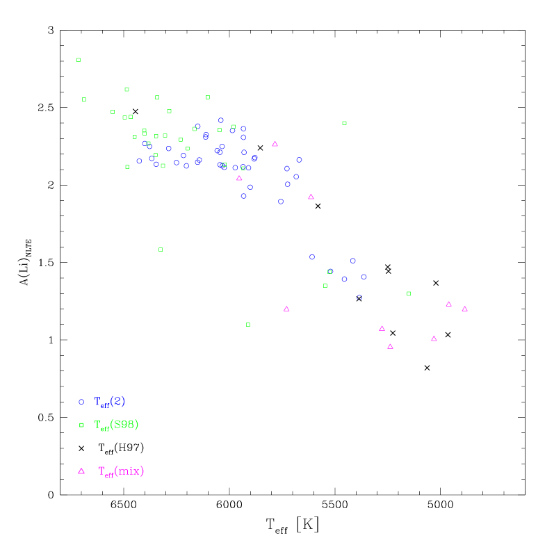
Figure 12: Lithium abundances as determined by using the sets of temperatures ${\rm T}_{\rm eff}$ (2) and ${\rm T}_{\rm eff}$ (S98) for the clean sample (half-half, circle and square symbols respectively), ${\rm T}_{\rm eff}$ (H97) and ${\rm T}_{\rm eff}$ (mix) for the $\beta$ and ubvy sample (crosses and triangles respectively), in the attempt of mimicking a common situation in which reddenings are taken from different sources

Still related to the determination of an accurate temperature scale, and as already seen in § 5, reddening plays an important role. For instance, R99 noted that their reddening estimates based on two different methods (Strömgren photometry and reddening maps) showed a clear discrepancy of about 0.02 mag, with the Strömgren-based E(b-y) values being higher despite the expected relationship E(B-V)$\simeq$1.35E(b-y). The solution chosen by these authors was to give higher weight to the maps-based reddening values based on the consideration that their targets were bright, hence a low intrinsic reddening might be expected. Therefore, they systematically lowered all the Strömgren-based E(b-y) values by 0.02 mag before averaging the two methods. As we do not know the final answer either, we cannot say if this is a good solution or not. At least for those objects we have in common these stars fall well outside the inner 50-70pc of the solar neighborhood (they span distances up to 1kpc), for which a low intrinsic reddening could be questionable.

Even more instructive is to evaluate the realistic situation in which one may refold on selecting reddening values from different sources, such as InfraRed dust maps and/or from the literature, because one method alone cannot be applied homogeneously to the entire sample under investigation. Keeping in mind that the exact details of such situation are very difficult to foresee, hence to reproduce, we tried to mimick such case by plotting a mix of lithium abundances: Fig. 12 shows A(Li)_NLTE versus ${\rm T}_{\rm eff}$ , where the lithium abundances were derived by selecting ${\rm T}_{\rm eff}$ (2) and ${\rm T}_{\rm eff}$ (S98) for the clean sample (half-half), and ${\rm T}_{\rm eff}$ (H97) and ${\rm T}_{\rm eff}$ (mix) for the $\beta$ and ubvy samples respectively. This likely represents an extreme case, but it certainly gives an idea of what effect could be expected. Also, please note that the A(Li) values corresponding to ${\rm T}_{\rm eff}$ (mix) were computed only for those stars for which this solution was applied (cf § 5.1 and § 5.2).

In summary, despite the seeming convergence at least on the absence of dispersion, the finding of discordant results is not surprising if some (or all) of the above-mentioned points are kept in mind. At the moment the only claim for a tilted A(Li)_NLTE-plateau is with metallicity, but most “metallicities” quoted in the literature are still derived from neutral iron lines, the formation of which is subject to NLTE conditions. Furthermore, R99 (as well as our work) have used metallicity values extracted from a careful inspection of the literature, which does not guarantee the homogeneity required for discussing the A(Li) vs [Fe/H] trend. Since the whole discussion of a possible slope of the lithium plateau with metallicity is centred on a small dependence, we encourage future analyses of Li abundances to determine the metallicities spectroscopically, possibly from Fe II lines (insensitive to NLTE effects).

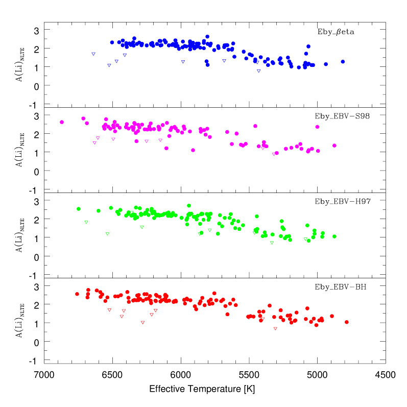
Figure 13: Lithium abundances computed with four different sets of temperatures as derived by using different reddening estimates (as reported in the upper right corner of each pan). Upside-down open triangles represent abundance upper limits.

8 Preliminary results on the mean lithium abundance and the dispersion

8.1 Last words of caution before further analysis

A first visual comparison of the different A(Li)_NLTE abundances we have derived for each star is presented in Fig. 13, where the first three (from the top) panels show how differently the plateau may appear when the lithium abundance has been derived from a different set of temperatures. The bottom pan is shown only for comparison purposes, and represents the A(Li)_NLTE abundances as derived from photometry that has been dereddened using the BH H i maps. Figure 13 shows how claims of dispersion or lack thereof from the same data-sample are perfectly plausible (see also our discussion in § 7).

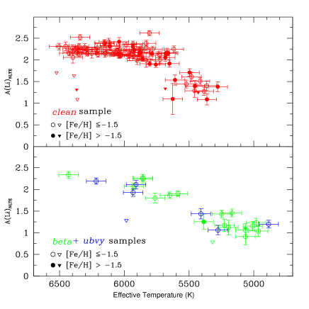
Figure 14: Final lithium abundances with associated 1$\sigma$-errorbars as a function of effective temperature (using ${\rm T}_{\rm eff}$ (2)) are shown for our clean sample (top) and beta $+$ ubvy samples (bottom)

In addition, since our complete sample is a non-homogeneous sample (because of the compromises made on the derivation of the effective temperature for some of the stars), any discussion of the width and slope of the A(Li)-plateau requires the separation of the complete sample into the clean, $\beta$, and ubvy sub-samples. In Figs. 14 and 15, we plot the A(Li)_NLTE values vs our ${\rm T}_{\rm eff}$  scale (i.e. ${\rm T}_{\rm eff}$ (2)) and [Fe/H] respectively, with the clean sample always plotted in the top panel and the $\beta$ and ubvy samples in the lower panel. Moreover, open symbols refer to objects with [Fe/H]$\leq-$1.5 in Fig. 14 and ${\rm T}_{\rm eff}$ $\geq$5700 K in Fig.15, and filled symbols represent respectively stars with [Fe/H]$>-$1.5 and ${\rm T}_{\rm eff}$ $<$5700 K. Upside-down triangles always identify abundance upper limits.

In the rest of the paper, we give our results regarding the characteristics of the plateau for the clean sample on one hand, and for the complete (i.e., clean + $\beta$ + ubvy) sample on the other hand. Additionally, we will consider as “plateau stars” those with ${\rm T}_{\rm eff}$ $\geq 5700$ K and [Fe/H]$\leq-1.5$. The metallicity limit is taken in order to avoid any contamination by lithium production from the various possible stellar sources (e.g., Travaglio et al. 2001). The cutoff in ${\rm T}_{\rm eff}$ is chosen for comparison reasons with previous analyses in the literature. However for the purposes of constraining stellar evolution models we will also discuss the cases where the lower limit in ${\rm T}_{\rm eff}$ is increased to 6000 K in order to avoid proto-stellar lithium destruction (in the case of the dwarfs, see § 10) or dilution at the very beginning of the first dredge-up phase (in the case of the post-turnoff stars, see § 11). Our results will be given considering the stars with lithium abundance determinations only, the case of stars with upper limits being considered separately in § 13.

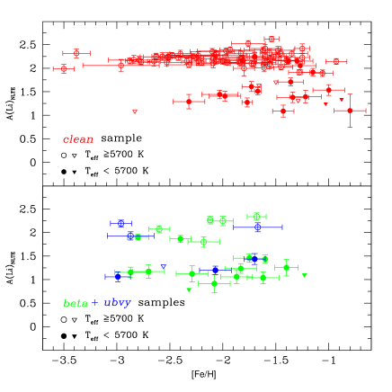
Figure 15: Final lithium abundances with associated 1$\sigma$-errorbars as a function of metallicity (using ${\rm T}_{\rm eff}$ (2)) are shown for our clean sample (top) and for our beta $+$ ubvy samples (bottom)

8.2 The mean lithium plateau abundance

Considering the stars with [Fe/H]$\leq-1.5$ and in the case of the most relaxed ${\rm T}_{\rm eff}$   lower limit (5700 K, cf Figs. 14 and 15) we obtain

$$A(Li)_{NLTE}=2.2138\pm 0.0929$$

and

$$A(Li)_{NLTE}=2.2080\pm 0.0947$$

for the clean and complete samples respectively, with rms values of 0.0587 and 0.0530. This is compatible with a normal distribution (i.e., as would be expected from the observational errors).

For the stars with ${\rm T}_{\rm eff}$ $\geq$6000 K, we find a mean lithium abundance of

$$A(Li)_{NLTE}=2.2243\pm 0.0748$$

for the clean sample, and of

$$A(Li)_{NLTE}=2.2368\pm 0.0840$$

for the complete sample. In both cases the dispersion values are slightly higher than the rms of the estimated observational error (0.0587), but compatible with no dispersion on the plateau.

Similar conclusions on dispersion can be drawn if no lower limit on [Fe/H] (in our specific case this was set to $-$2.1) is assumed in the ${\rm T}_{\rm eff}$ -(b-y)_o calibration (see § 5 for more details). The higher effective temperatures thus derived and shown in Fig. 3 would have the only effect of increasing our mean A(Li) plateau values by 0.025-0.035 dex.

We would like to note that the 6 stars that could be moved to the ubvy sample (if we were to consider a 3 digit precision on $\beta$, cf end of § 5.2) are not relevant in the final discussion of the Li plateau spread as they are cool stars that have their lithium already depleted (5 of them) or a normal plateau lithium abundance (1 star with A(Li)_NLTE=2.22).

The absence of intrinsic dispersion that we get is in agreement with the results of Molaro et al. (1995), Spite et al. (1996), Bonifacio & Molaro (1997), Ryan et al. (1999) and Meléndez & Ramírez (2004).

Furthermore, because all these works (ours included) find quite consistent A(Li) plateau values (note that the apparently higher plateau value found by Meléndez & Ramírez (2004, A(Li)_NLTE=2.37) should be corrected downwards by 0.08 dex because of the different Kurucz model atmospheres employed in their and our study, making it then in closer agreement with our findings), it seems that in general the relatively low lithium abundance (when compared to the CMB+SBBN result) seen in metal poor halo stars is a very robust result. Assuming the correctness of the CMB constraint on the value of the baryon-to-photon ratio we are then left with the conclusion that the Li abundance seen at the surface of halo stars is not the pristine one, but that these stars have undergone surface lithium depletion at some point during their evolution.

Let us try now to look for some constraints on the depletion mechanism(s).

9 Evolutionary status of the stars

Using the data we have gathered and homogenized in the first part of this paper, we will now look at the Li plateau by adding one extra dimension to the problem, namely by considering the evolutionary status of each star of our complete sample. Indeed not all our objects are dwarf stars. The contamination from evolved stars has thus to be evaluated in order to precisely determine the lithium abundance along the plateau and to look for the trends and for the depletion factor.

9.1 Input quantities

We use the HIPPARCOS (ESA 1997) trigonometric parallax measurements to locate precisely our objects in the HR diagram. Among the 118 stars of our complete sample, 3 objects (HIP 484, 48444, and 55852) have spurious Hipparcos parallaxes, and are thus rejected from further analysis.

Intrinsic absolute magnitudes M_V are derived from the m_V and the parallaxes given in the Hipparcos catalogue. We determine the bolometric corrections BC by using the relations between BC and V-I (these quantities being also taken from the Hipparcos catalogue) given by Lejeune et al. (1998) and which are metallicity-dependent. We use the values of [Fe/H] derived in our final analysis (Table 6, column 2). We first iterate using the log $g$  values available in the literature, and finally attribute to our stars the log $g$  value derived from their position in the HR diagram (Table 9, column 10). Finally, we compute the stellar luminosity and the associated error from the one sigma error on the parallax. All the relevant quantities are given in Tables 8 and 9.

Table 8: Quantities extracted from the HIPPARCOS catalogue for our sample stars ((B-V) and E(B-V) are given in Table 4). The whole table is available on-line

HIP	V	Plx	e$\_$Plx	d	VI
	mag	(mas)	(mas)	(pc)
911	11.80	6.13	5.67	163	0.64
3026	9.25	9.57	1.38	104	0.54
3446	12.10	15.15	3.24	66	0.58
3564	10.60	2.07	2.16	483	0.67
8572	10.34	3.22	1.75	310	0.50
…	…	…	…	…	…

9.2 Determination of the stellar evolutionary status

The resulting HR diagrams are shown in Fig. 16 for our complete sample split in four metallicity bins. The evolutionary status of each star has been determined on the basis of these HR diagrams, and is given in Table 9. Each star has been assigned to one of the following sub-classes: 5 identifies the dwarfs (i.e., main-sequence stars), 4.5 stands for the turnoff stars, 4 for the subgiants (i.e., stars crossing the Hertzsprung gap), 3.5 for the stars at the base of the RGB, and 3 for the stars on the RGB. “Post-main sequence stars” can be easily located on the HRD (see Fig. 16) as those stars with Log(L/L_⊙) higher than $\sim$ 0.4. In this luminosity range, we identify as turnoff and subgiant stars those with ${\rm T}_{\rm eff}$ $\geq$ 5600 K, whereas cooler stars are classified as “base RGB” or RGB stars depending on their luminosity. This limit in effective temperature is chosen because it corresponds to the approximate value where lithium dilution is expected to occur at the very beginning of the first dredge-up (i.e., Deliyannis et al. 1990, Charbonnel 1995). The distribution in these sub-classes is given in Table 10. For most of our objects, the classification was performed unambiguously. Some stars (21 in total) were first classified as “unsure”, the uncertainty being due to the large errorbar on the derived luminosity inherited from the error on the Hipparcos parallax (see Fig. 16). However, by cross-checking the luminosity and the corresponding gravity obtained from Hipparcos data with the M_V and gravity values quoted in the literature, we were able to attribute a relatively certain evolutionary status (given in the last row of Table 10) to all these objects, thus keeping them in our statistical analysis. As a result, the clean sample (respectively the complete sample) contains 49 (59) dwarfs, 5 (5) turnoff stars, 29 (31) subgiants, 5 (18) base RGB stars and 2 (5) RGB stars.

Table 9: Characteristics and evolutionary status of the sample stars. The whole table is available on-line

HIP	MV	MV	BC	Mbol	Log(${{L}\over{L_{\odot}}})$	Log(${{L}\over{L_{\odot}}})$	e$\_$Log(${{L}\over{L_{\odot}}})$	log g	statuss
		dered				dered
911	5.74	5.74	-0.176	5.56	-0.32	-0.32	0.80	4.50	5
3026	4.15	4.15	-0.169	3.99	0.31	0.31	0.13	3.85	5
3446	8.00	8.00	-0.085	7.92	-1.27	-1.27	0.19	4.50	5
3564	2.18	2.06	-0.221	1.96	1.12	1.17	0.91	3.50	4
8572	2.88	2.79	-0.112	2.77	0.79	0.83	0.47	3.85	4
…	…	…	…	…	…	…	…	…	…

(s) Status : 5:dwarf - 4.5:turnoff - 4:subgiant - 3.5:base RGB - 3:RGB

(see the text for more details on the adopted definitions of these statuses)

In Fig. 17 we plot A(Li)_NLTE vs ${\rm T}_{\rm eff}$ for four metallicity bins and indicate the evolutionary status of the stars by different symbols. It is interesting to note that for [Fe/H]$\leq-$2, all the coolest stars (i.e., with ${\rm T}_{\rm eff}$ $\leq$ 5500 K) are actually evolved stars (see also Fig. 18). This fact must be taken into account when comparing stellar evolution models and observations. In the [Fe/H] range between $-$2 and $-$1.5, the decrease of lithium relative to the plateau dwarf stars appears at $\sim$ 5600 - 5700 K.

9.3 Comparison with previous work

In their careful analysis of the classical mechanisms that could alter the surface Li abundance of halo stars at different phases of their evolution, Deliyannis et al. (1990, hereafter D90) focused on the separation of the halo population into pre- and post-turnoff groups as an essential prerequisite to understand the Li observations. At that time they considered a limited sample of halo stars. They used the trigonometric parallaxes and V-colors from the Yale Parallax Catalogue (van Altena et al. 1989) when available to determine M_V; otherwise M_V was taken from the original observational papers. We have 36 objects in common with D90’s sample. For 19 of them the same evolutionary status has been attributed in both D90 and our study. However 13 of the stars which were identified as “pre-turnoff” objects by D90 appear to be more evolved stars on the basis of their more precise and reliable Hipparcos parallaxes. Conversely 4 out of the 7 stars which were claimed to be “post-turnoff” objects in D90’s study are dwarf stars.

Ryan & Deliyannis (1998) took advantage of the Hipparcos parallaxes (when available) in order to separate their sample of halo stars cooler than the plateau into dwarf and subgiant classes. The 14 stars that we have in common with their sample have been attributed the same evolutionary status in both analyses (theirs and ours).

Note that our definition of a subgiant is different and more strict, as far as the effective temperature range is concerned, than the one adopted by PSB93, who studied the lithium abundances for 79 so-called halo subgiants. PSB93 constructed their sample on the basis of ubvy photometry (more precisely from their location in the c₁ vs (b-y) plane) from several catalogs of metal-poor stars. Hipparcos parallaxes are now available for almost all their objects, allowing a more precise determination of their location in the HRD. In the present study we did not consider the most evolved stars of PSB93’s sample, i.e., those with ${\rm T}_{\rm eff}$ below 4800 K. These objects indeed experience some extra-mixing beyond the first dredge-up and lose then all the information about their initial lithium content (see Charbonnel 1995; Weiss & Charbonnel 2004). They are thus of no help in discussing the initial lithium content.

Table 10: Distribution of the evolutionary status in our different sub-classes. The last line indicates the status that we could attribute to the stars which were first labelled as “unsure” (see the text for more details)

	Sample
	Clean	Polluted (beta+ubvy)
total	90	27(20+7)
dwarfs	44	10(6+4)
turnoff	3	0
subgiant	18	2(1+1)
base RGB	5	13(11+2)
RGB	1	0
unsure	19	2 (2+0)
	[5dw, 2to, 11sg, 1rgb]	[1dw, 1rgb]

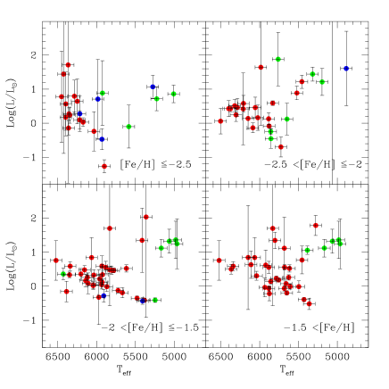
Figure 16: HR diagram for our complete sample stars for separate metallicity bins (using ${\rm T}_{\rm eff}$ (2))

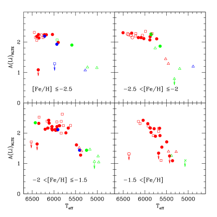
Figure 17: A(Li)_NLTE versus ${\rm T}_{\rm eff}$ (2) for our complete sample stars, for separate metallicity bins. The different symbols indicate the evolutionary status of the stars. Filled circles : dwarfs. Open circles : turnoff stars. Open squares : subgiants. Open triangles : stars at the base of the RGB. Crosses : RGB stars. The arrows indicate the lithium upper limits

10 The lithium abundance along the plateau for the dwarf stars

We now concentrate our analysis on the dwarf stars. Their lithium abundance is plotted in Fig. 18.

10.1 The analytical method

For the reasons given in § 8.1, we identify as “plateau stars” those with [Fe/H]$\leq-1.5$ and with ${\rm T}_{\rm eff}$ higher than 5700 or 6000 K. The corresponding numbers of stars in each bin is given in Table 11. For the time being, we keep in our analysis the possible binary stars (but see § 12), but we eliminate the stars with lithium upper limits, that will be discussed separetely in § 13. We note that in the metallicity and effective temperature ranges we have chosen to define the plateau only two dwarf stars of the clean sample have Li upper limits, namely HIP 72561 and 100682. With A(Li)_NLTE $\leq$ 1.639 and $\leq$ 1.088 respectively (with [Fe/H] = $-$1.66 and $-$2.83, ${\rm T}_{\rm eff}$ = 6388 and 6362 K), both stars fall well below the plateau (see Fig. 18).

Table 11: Number of dwarfs in each subsample

[Fe/H]	Clean	Polluted	Clean	Polluted
		(beta+ubvy)		(beta+ubvy)
	$>$5700	$>$5700	$>$6000	$>$6000
$\leq$-2.5	8	0+2	7	0+1
-2.5 to -2.0	9	2+0	6	0+0
-2.0 to -1.5	16	1+1	9	1+0

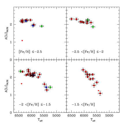
Figure 18: A(Li)_NLTE versus ${\rm T}_{\rm eff}$ (2) for the dwarfs of our complete sample. Upside-down triangles represent lithium upper limits

In order to investigate the existence of trends in the [A(Li)_NLTE, ${\rm T}_{\rm eff}$ ] and [A(Li)_NLTE,[Fe/H]] planes we performed univariate fits by means of four estimators : (1) The least-squares fit with errors in the independant variable only (routine FIT of Press et al. 1982); (2) The least-squares fit with errors in both variables (routine FITEXY of Press et al. 1982); (3) The BCES (bivariate correlated errors and intrinsic scatter) of Akritas & Bershady (1996); (4) BCES simulations bootstrap based on 10000 samples. All univariate fits in the A(Li)_NLTE versus ${\rm T}_{\rm eff}$ plane were computed considering an error on ${\rm T}_{\rm eff}$ of both 75 and 100 K.

10.2 Mean value and dispersion

Table 12: Average value of A(Li)_NLTE, average and standard deviation, and rms for the dwarf stars : mean${}^{\pm{\rm aver}}_{\pm{\rm stand}}$ (rms). We separate the clean and the complete sample and give the results for 2 limits in effective temperature

[Fe/H]	${\rm T}_{\rm eff}$ $\geq$5700 K
	clean	complete
$\leq$-2.5	2.183${}^{\pm 0.070}_{\pm 0.097}$ (0.042)	2.156${}^{\pm 0.093}_{\pm 0.119}$ (0.052)
-2.5 to -2.0	2.170${}^{\pm 0.067}_{\pm 0.087}$ (0.047)	2.187${}^{\pm 0.072}_{\pm 0.085}$ (0.057)
-2.0 to -1.5	2.178${}^{\pm 0.088}_{\pm 0.109}$ (0.042)	2.183${}^{\pm 0.092}_{\pm 0.111}$ (0.067)
$\leq$-1.5	2.177${}^{\pm 0.071}_{\pm 0.098}$ (0.047)	2.177${}^{\pm 0.084}_{\pm 0.104}$ (0.052)
	${\rm T}_{\rm eff}$ $\geq$6000 K
	clean	complete
$\leq$-2.5	2.216${}^{\pm 0.038}_{\pm 0.047}$ (0.042)	2.212${}^{\pm 0.037}_{\pm 0.044}$ (0.052)
-2.5 to -2.0	2.202${}^{\pm 0.079}_{\pm 0.091}$ (0.047)	2.202${}^{\pm 0.079}_{\pm 0.091}$ (0.047)
-2.0 to -1.5	2.225${}^{\pm 0.088}_{\pm 0.108}$ (0.042)	2.236 ${}^{\pm 0.100}_{\pm 0.115}$(0.067)
$\leq$-1.5	2.215${}^{\pm 0.074}_{\pm 0.088}$ (0.047)	2.200${}^{\pm 0.074}_{\pm 0.088}$ (0.052)

The average value of the lithium abundance is given in Table 12, together with the average, standard deviation and root mean square of the estimated observational errors for several subsets of data (in terms of metallicity and effective temperature intervals, as well as in terms of clean vs complete samples) of the dwarf sample.

If we consider the entire metallicity range [Fe/H]$\leq-$1.5, the straight average value of the lithium abundance for the plateau dwarf stars with ${\rm T}_{\rm eff}$ $\geq 5700$ K is

$$A(Li)_{NLTE}=2.1768\pm 0.0711$$

and

$$A(Li)_{NLTE}=2.1773\pm 0.0840$$

for the clean and complete samples respectively. The average dispersion is small, but slightly higher than the respective rms of 0.0474 and 0.0516.

When we restrict our analysis to the dwarf stars with ${\rm T}_{\rm eff}$ $\geq 6000$ K, the mean value increases to

$$A(Li)_{NLTE}=2.2154\pm 0.0737$$

and

$$A(Li)_{NLTE}=2.2200\pm 0.0740$$

for the clean and the complete samples respectively. Again the average dispersion is small but slightly higher than the rms (0.0474 and 0.0516 respectively).

We thus find no evidence of an intrinsic dispersion in the Li abundances along the plateau. As expected, this result which was already presented in § 8.2, is now reinforced having eliminated the “pollution” by evolved stars and focussed on the dwarf stars only.

As we already mentioned in § 8.2, the assumption of a lower limit on [Fe/H] in our ${\rm T}_{\rm eff}$ -(b-y)_o calibration does not affect our conclusions on dispersion. The only effect when one does not consider this limit is to increase the mean A(Li) value of the dwarf sample by less than 0.02 dex for the entire metallicity range. If we consider only our most metal-poor subsamples the increase in the mean A(Li) value is of course slightly higher (from 0.02 up 0.08 dex depending on the lowest limit on ${\rm T}_{\rm eff}$ used for the plateau definition).

The mean lithium values for the dwarf stars are slightly lower, although fully compatible within the quoted errors, than the mean values given in § 8.2 for the entire sample of stars (i.e., that in which we did not discriminate the stars according to their evolutionary status). This point will be discussed at length in § 11.

10.3 The A(Li)_NLTE versus ${\rm T}_{\rm eff}$ correlation

When we consider the dwarfs with ${\rm T}_{\rm eff}$ $\geq$ 5700 K and [Fe/H]$\leq-$1.5, we find a small slope in the A(Li)_NLTE-${\rm T}_{\rm eff}$ plane of

$$0.019/100\leavevmode\nobreak\ K\leavevmode\nobreak\ {\rm and}\leavevmode\nobreak\ 0.028/100\leavevmode\nobreak\ K$$

for the clean and complete samples respectively. These numbers are obtained when we use our standard error on ${\rm T}_{\rm eff}$ of 75 K. In the more conservative case of an error on ${\rm T}_{\rm eff}$ of 100 K, we get respectively 0.026/100 K and 0.033/100 K.

This is very similar to the slope found by BM97 of 0.02/100 K, and slightly lower than those found by Thorburn (1994) of 0.034/100 K and by R96 of 0.0408/100 K. On the contrary, Meléndez & Ramírez (2004) do not find any dependence of A(Li) on either ${\rm T}_{\rm eff}$  or [Fe/H].

In order to focus on the physical processes that may affect the surface lithium abundance only when the stars are on the main sequence (in other words, to avoid any pre-main sequence depletion; see e.g. D90, Richard et al. 2004) we made the same computations for the stars with ${\rm T}_{\rm eff}$ $\geq$ 6000 K. In this case and for the whole [Fe/H]$\leq-$1.5 range, we get a slightly smaller slope, i.e.

$$0.015/100\leavevmode\nobreak\ K$$

for the clean sample and a very similar slope, i.e.

$$0.029/100\leavevmode\nobreak\ K$$

for the complete sample, assuming an error on ${\rm T}_{\rm eff}$ of 75 K. When we consider an error on ${\rm T}_{\rm eff}$ of 100 K, we get respectively 0.027/100 K and 0.041/100 K.

We note that if we split the [Fe/H] interval as done for example in Fig. 18, we find a negative slope of $\sim-$ 0.025 for the stars with [Fe/H]$\leq-$2.5, both for the clean and complete samples for the stars with ${\rm T}_{\rm eff}$ $\geq$ 6000 K. Small but positive slopes are detected when we look at the $-$2.5 $<$ [Fe/H]$\leq-$2.0 and $-$2.0 $<$ [Fe/H]$\leq-$1.5 intervals.

10.4 The A(Li)_NLTE versus [Fe/H] correlation

In Fig. 19 we plot A(Li)_NLTE vs [Fe/H] for the plateau dwarfs of our entire sample but we look for trends up to [Fe/H] = -1.5 only. The highest slope ($\sim$ 0.05 up to [Fe/H] = -1.5) is obtained for the most extended sample, i.e., for the dwarf stars of the complete sample with ${\rm T}_{\rm eff}$ $\geq$ 5700 K, whereas when we consider only the dwarf stars of the clean sample (still with ${\rm T}_{\rm eff}$ $\geq$ 5700 K) the correlation becomes slightly flatter (the slope is $\sim$ 0.02). When we focus on the dwarf stars with ${\rm T}_{\rm eff}$ $\geq$ 6000 K, the dependence of A(Li) with metallicity remains small (with a slope of $\sim$ 0.03 and 0.02 dex up to [Fe/H] = -1.5 for the complete and clean samples respectively). In Fig. 19 we also show the values when no lower limit on [Fe/H] is assumed in the ${\rm T}_{\rm eff}$ -(b-y)₀ calibration. A slightly lower slope would have been derived under this assumption.

Our results are intermediate between those of BM97 ($-$0.05 to 0.00, i.e., no slope) and those of R99 (+0.118) and Thorburn (1994; +0.13). We note that the preliminary results of Asplund et al. (2005) indicate a dependence of A(Li) on metallicity (the latter computed both as the abundance of iron and oxygen), characterised by a slope of 0.10.

We remind the reader that lithium synthesis by galactic cosmic rays (GCR) leads indeed to an increase of its abundance with metallicity, but this contribution safely can be considered small up to [Fe/H]=$-$1.5 (Molaro et al. 1997) in agreement with our finding. This can be estimated using the observed correlation between ⁹Be and metallicity together with the Li/Be ratio predicted by GCR theory (Walker et al. 1985).

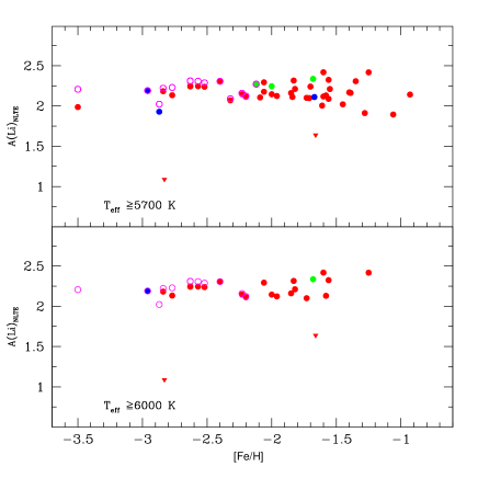
Figure 19: A(Li)_NLTE versus [Fe/H] only for the dwarfs with ${\rm T}_{\rm eff}$ $\geq 5700$ K (upper figure) and with ${\rm T}_{\rm eff}$ $\geq 6000$ K (lower figure) of our entire sample. Upside-down triangles represent abundance upper limits. The open circles correspond to the case where no lower limit on [Fe/H] is assumed in the colour-${\rm T}_{\rm eff}$ calibration, while the others correspond to the case where this limit is set to -2.1

As discussed already in §7.2, the trends with metallicity here derived must be taken with caution, as we have gathered our metallicities from the literature. This does not guarantee the homogeneity required for an accurate study of the metallicity dependence. Additionally such an analysis would require homogeneous spectroscopic determinations from Fe II lines insensitive to NLTE effects rather than from neutral iron lines as it is the case for most of the currently available Li analyses (hence also for our values). For these reasons we will not continue the discussion nor derive any conclusions on the lithium-metallicity relation.

10.5 The dwarf stars cooler than the plateau

As already mentioned in § 9.2, the current sample does not contain cool (i.e., with ${\rm T}_{\rm eff}$ $\leq$ 5500 K) dwarf stars at low-metallicity (i.e., [Fe/H] $\leq-$ 2). This is the first surprise of our check on the evolutionary status of our sample stars. It thus appears that for the cooler and more metal-deficient dwarfs we have no direct clue to the lithium behavior. We expect these objects to exhibit the same pattern as that seen in cool open cluster and Pop I field stars as well as in our sample stars at higher metallicity (bottom panels of Fig. 18), although this remains to be confirmed observationally. In the [Fe/H] range between $-$2 and $-$1.5, substantial lithium depletion relative to the plateau value sets in at $\sim$ 5600 – 5700 K. Between 5700 and 5100 K, the lithium depletion slope is $\sim$ 0.21 dex per 100 K.

11 The lithium abundance in evolved stars

We now address the case of more evolved stars. Their lithium abundance is plotted in Fig. 20 for four metallicity bins as a function of ${\rm T}_{\rm eff}$ which is now an indicator of the evolutionary status. We analyse the lithium behaviour in two separate groups of objects: turnoff and subgiant stars on one hand, and RGB stars on the other hand. We compare our results with the lithium data in globular clusters.

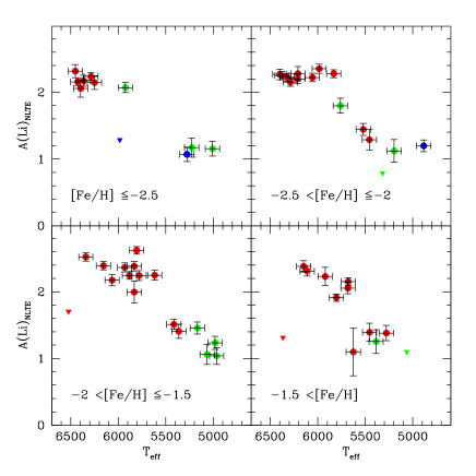
Figure 20: A(Li)_NLTE versus ${\rm T}_{\rm eff}$ (2) for the turnoff and more evolved stars of our entire sample for four metallicity bins. Triangles are for lithium upper limits. Effective temperature is here an indicator of the evolutionary status of the stars

11.1 The mean lithium value in turnoff and subgiant stars

Table 13: Straight average value of A(Li)_NLTE, average and standard deviation for the turnoff and subgiant stars : mean${}^{\pm{\rm aver}}_{\pm{\rm stand}}$ (rms). We separate the clean and the complete samples and present the results for 2 limits in effective temperature

[Fe/H] interval	${\rm T}_{\rm eff}$ $\geq$5700 K
	clean	complete
$\leq$-2.5	2.180${}^{\pm 0.064}_{\pm 0.088}$ (0.093)	2.164${}^{\pm 0.066}_{\pm 0.090}$ (0.053)
-2.5 to -2.0	2.253${}^{\pm 0.045}_{\pm 0.058}$ (0.075)	2.247${}^{\pm 0.042}_{\pm 0.057}$ (0.075)
-2.0 to -1.5	2.326${}^{\pm 0.144}_{\pm 0.187}$ (0.059)	2.326${}^{\pm 0.144}_{\pm 0.187}$ (0.059)
$\leq$-1.5	2.260${}^{\pm 0.098}_{\pm 0.136}$ (0.059)	2.252${}^{\pm 0.099}_{\pm 0.138}$ (0.053)
	${\rm T}_{\rm eff}$ $\geq$6000 K
	clean	complete
$\leq$-2.5	2.180${}^{\pm 0.064}_{\pm 0.088}$ (0.093)	2.180${}^{\pm 0.064}_{\pm 0.088}$ (0.093)
-2.5 to -2.0	2.232${}^{\pm 0.033}_{\pm 0.046}$ (0.075)	2.227${}^{\pm 0.032}_{\pm 0.043}$ (0.075)
-2.0 to -1.5	2.362${}^{\pm 0.126}_{\pm 0.176}$ (0.059)	2.362${}^{\pm 0.126}_{\pm 0.176}$ (0.059)
$\leq$-1.5	2.235${}^{\pm 0.077}_{\pm 0.109}$ (0.059)	2.235${}^{\pm 0.077}_{\pm 0.109}$ (0.059)

As already mentioned in § 10, we put a lower limit on the effective temperature (5700 and 6000 K) for our analysis, this time in order to avoid any lithium depletion due to the first dredge-up. We consider stars both at the turnoff and on the subgiant branch as defined in § 9.2. Two stars are excluded from the analysis, namely HIP 81276 ([Fe/H] = $-$1.50, ${\rm T}_{\rm eff}$  = 6523 K) of the clean sample and HIP 83320 ([Fe/H] = $-$2.56, ${\rm T}_{\rm eff}$  = 5984 K) of the ubvy sample, because of their A(Li)_NLTE upper limits (of 1.705 and 1.287 respectively, see Fig. 20). The average value of A(Li)_NLTE, the average and standard deviation and the root mean square of the observational errors are given in Table 13 for various metallicity and effective temperature intervals and for the clean and complete samples.

A very surprising result emerges here for the first time: Whatever the subsample we consider (i.e., clean or complete sample, ${\rm T}_{\rm eff}$ $\geq$ 5700 or 6000 K), the mean value of A(Li)_NLTE always appears to be higher for the subgiant stars than for the dwarfs, except for the most metal-deficient objects (i.e., with [Fe/H]$\leq-$2.5) where the mean lithium abundance is very similar in both evolutionary statuses.

In the case of the evolved stars with ${\rm T}_{\rm eff}$ $\geq$ 5700 K and [Fe/H]$\leq-$1.5,

$$A(Li)_{NLTE}=2.2599\pm 0.0997$$

and

$$2.2524\pm 0.0990$$

for the clean and complete samples respectively. These values have to be compared respectively with 2.1768$\pm$0.0711 and 2.1773$\pm$0.0840 for the dwarfs the same range of effective temperature.

When we restrict our inspection to the stars with ${\rm T}_{\rm eff}$ $\geq$ 6000 K and [Fe/H]$\leq-$1.5, the mean value of A(Li)_NLTE for the evolved stars is

$$2.2349\pm 0.0769$$

for both the clean and the complete samples, which has to be compared with 2.2154$\pm$0.0737 and 2.2200$\pm$0.0740 for the dwarf stars.

Once again, we note that our conclusions are not affected by having assumed $-$2.1 as the lower limit on the metallicity to be used in our colour-${\rm T}_{\rm eff}$  calibration (see § 5). The only effect of not considering this limit would be a slight increase of the Li mean value by $\sim$0.04-0.05 dex.

Although the numbers for the dwarf and evolved stars are fully compatible within the quoted errors, the difference between the mean lithium values of both populations is stricking. As already discussed in § 7.1, the dependence of the lithium abundance on gravity is weaker than that on effective temperature. At ${\rm T}_{\rm eff}$  = 6000 K and [Fe/H] = $-$1.5, the typical effect is at most +/$-$0.01 dex in A(Li) for $-$/+1 dex in log $g$. We can thus see that even an error of 1 dex on the attributed gravity (which is very unlikely in view of the good precision of the Hipparcos parallax for most of the stars) cannot explain the difference on the mean lithium abundance that we obtain between the dwarf and subgiant stars. Neither can the dependence of our colour-${\rm T}_{\rm eff}$  calibration on log $g$. There is indeed a dependence for giant stars because (b-y) measures the slope of the Paschen continuum, which in turn is affected by a change downwards of the gravity (cf RM05b). However, what we call “evolved” stars are objects that have just passed the turn-off or that are located on the subgiant branch: they are not real giants, as defined in RM05b.

11.2 Dispersion in evolved stars

Our analysis reaveals another remarkable feature: Post-main sequence Population II stars appear to exhibit a non negligible Li dispersion. As can be seen for example in Fig.20, this is already true at the turnoff and all along the evolution traced by the effective temperature.

For the subgiants near 6000 K, PSB93 found a small spread in the lithium abundance around a mean value of 2.1. We see from the previously quoted numbers that the dispersion is actually not negligible in our sample of slightly evolved stars, independently of the adopted limit in effective temperature (5700 or 6000 K).

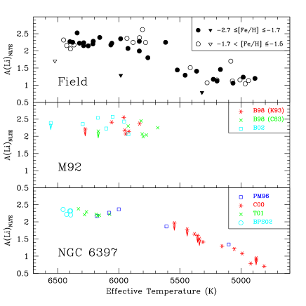
Figure 21: Lithium abundance versus ${\rm T}_{\rm eff}$ for the turnoff and more evolved stars of our sample (upper panel, ${\rm T}_{\rm eff}$ (2)) and for their counterparts in the globular clusters M92 and NGC 6397 (lower and middle panel respectively). Effective temperature is here an indicator of the evolutionary status of the stars. For the field stars we focus on our sample stars in a limited metallicity range around that of the two globular clusters discussed here ([Fe/H] = $-$2.52 for M92, King et al. 1998; [Fe/H] = $-$2.02 for NGC 6397, Thévenin et al. 2001). All the Li values are NLTE (see the text). For M92, the original data are from Boesgaard et al. (1998, B98) and Bonifacio (2002, B02). For B98 study we plot the data both on the Carney (1983, C83) and King (1993, K93) temperature scales. The data for NGC 6397 are from Pasquini & Molaro (1996, PM96), Castilho et al. (2000, C00), Thévenin et al. (2001, T01) and Bonifacio et al. (2002, BPS02)

For the more evolved (i.e., cooler) stars, the lithium abundance is expected to decrease due to the first dredge-up at the effective temperature of $\sim$ 5700 K, this dilution episode being completed around 5200 K (i.e., Deliyannis et al. 1990, Charbonnel 1995). This is what we observe, even though this region is not very well sampled. However if all the stars had left the main sequence with the same lithium content, they should share a common lithium abundance after the first dredge-up (remember that these stars have approximately the same initial mass). Instead, the evolved stars with ${\rm T}_{\rm eff}$ lower than $\sim$ 5500 K which have already undergone the first dredge-up dilution exhibit a relatively large lithium dispersion.

11.3 Comparison with globular cluster stars

The question of the lithium dispersion among metal-poor stars has already been discussed in the context of globular cluster studies. In Fig. 21 we show the data in the only two globular clusters for which Li abundances have been reported in stars down to the turnoff, namely M92 and NGC 6397 (middle and lower panel respectively). These are NLTE values, i.e. we corrected the LTE values reported in the literature for NLTE corrections which were computed following the same prescriptions we used for our field stars sample. Unfortunately, the unavailability of Strömgren photometry for all the globular cluster stars analysed in M92 and NGC6397 did not allow us to re-derive their lithium abundances based on our temperature scale. For M92 we rely on two analyses : i) Boesgaard et al. (1998, hereafter B98), from which we report the Li values for both temperature scales (Carney 1983, C83, and King 1993, K93) discussed in their original paper; ii) Bonifacio (2002, hereafter B02) which is based on B98 equivalent widths and on the temperature calibration by Bonifacio et al. (2002, hereafter BSP02). For NGC 6397, the Li abundances are taken from Pasquini & Molaro (1996), Castilho et al. (2000), Thévenin et al. (2001) and Bonifacio et al. (2002, BSP02). In Fig. 21 the globular cluster data are compared with the NLTE Li abundances of our evolved field stars in the metallicity range around that of the clusters ($-$2.7 $\leq$ [Fe/H] $\leq$ $-$1.7, black symbols in the upper panel).

B98 investigated the lithium abundance in seven stars near the turnoff of the old and metal-poor cluster M92 ([Fe/H] = $-$2.52, King et al. 1998). They reported a dispersion of a factor of $\sim$2.6 for the subgiant stars in a region around ${\rm T}_{\rm eff}$ $\sim$ 5800 K or 5950 K (depending on the adopted temperature scale, C83 or K93 respectively) as can be seen in the middle panel of Fig. 21. Contrary to B98, B02 concluded that there is no strong evidence for intrinsic dispersion in Li abundances among the M92 stars, although a dispersion as large as 0.18 dex is possible. B02 actually warned the reader that no definitive conclusion can be drawn on the intrinsic dispersion in this stellar cluster on the basis of the currently available spectra. Better observations with higher S/N ratios are still needed for these very faint M92 stars.

Although the data points are relatively scarce in this region, one sees from Fig. 21 that some dispersion indeed exists among field stars in the ${\rm T}_{\rm eff}$  range of B98’s data. The stars HIP 36430, 92775 and 102718 which have respectively [Fe/H] = $-$2.10, $-$2.18 and $-$1.80, ${\rm T}_{\rm eff}$  = 5985, 5762 and 5832 K, and very similar Log(L/L_⊙) = 1.69$\pm$1.71, 1.88$\pm$0.79 and 1.71$\pm$2.27, present significant differences in their NLTE-Li abundance : 2.352$\pm$0.068, 1.799$\pm$0.113 and 1.995$\pm$0.165. This corresponds to the dispersion claimed by B98 in M92. In addition at approximatively the same effective temperature the slightly more metal-poor star HIP 83320 ([Fe/H] = $-$2.56, ${\rm T}_{\rm eff}$  = 5984 K, Log(L/L_⊙) = 0.77$\pm$1.17) shows only an upper limit for Li (A(Li)$\leq$1.287). B98 discussed the case of the halo subgiant BD + 23^o3912 (HIP 99423) which was found by King et al. (1996) to have a remarkably high lithium abundance of 2.56$\pm$0.07. This star is also in our sample, with the following parameters : [Fe/H] = $-$1.54, ${\rm T}_{\rm eff}$  = 5806 K, and Log(L/L_⊙) = 0.48$\pm$0.12. We find a relatively high NLTE Li abundance of 2.620 for this object. Although its relatively high metallicity makes this star not very relevant when compared to M92 stars, we think that it reinforces the case for dispersion.

The lithium behavior in NGC 6397 ([Fe/H] = $-$2.02, Thévenin et al. 2001) is instead completely different: stars with ${\rm T}_{\rm eff}$ $\geq 6000$ K share the same lithium abundance with essentially no intrinsic scatter. No lithium abundance has been reported up to now in this cluster for stars over the $\sim$ 5600 to 6000 K range. Observations in this region would be useful.

12 Duplicity and variability

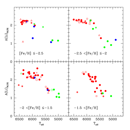
Figure 22: Duplicity and variability among our complete sample. Asterisks : confirmed single- or double-lined binaries (Latham et al. 2002, Carney et al. 2003, 1994). Open squares : stars marked as spectroscopic binaries in Bonifacio & Molaro (1997). Open triangles : suspected binaries (Latham et al. 2002). Crosses : binaries or stars in double/multiple system as reported in SIMBAD. Filled circles : single stars. Open circles : variable stars as reported in SIMBAD

Table 14: Average value of A(Li)_NLTE and average deviation for [Fe/H] $\leq$ -1.5 : When all the stars are considered regardless of their possible duplicity or variability (column a), when all the suspected and confirmed binaries are omitted (column b), and when only the confirmed binaries are excluded (column c). In cases (b) and (c) the stars reported as variable in SIMBAD are not considered. The first and second lines contain the values for the clean and the complete samples respectively

	(a)	(b)	(c)
dwarfs
Teff	2.177$\pm$0.071	2.184$\pm$0.098	2.186$\pm$0.092
$\leq 5700$ K	2.177$\pm$0.084	2.176$\pm$0.108	2.185$\pm$0.102
Teff	2.215$\pm$0.074	2.243$\pm$0.076	2.235$\pm$0.075
$\leq 6000$ K	2.220$\pm$0.074	2.257$\pm$0.075	2.253$\pm$0.074
turnoff and subgiant stars
Teff	2.260$\pm$0.098	2.297$\pm$0.119	2.307$\pm$0.127
$\leq 5700$ K	2.252$\pm$0.099	2.301$\pm$0.126	2.284$\pm$0.106
Teff	2.235$\pm$0.077	2.260$\pm$0.105	2.289$\pm$0.129
$\leq 6000$ K	2.235$\pm$0.077	2.260$\pm$0.105	2.253$\pm$0.085

After a careful inspection of the literature in order to identify single- and double-lined binaries (we mainly used the extensive surveys and listings by Latham et al. 2002, Carney et al. 1994,2003) we then tested if any of our above conclusions on the mean lithium abundance and on the dispersion may have been affected by the inclusion of binary stars. This is especially important because the literature-based EW values may have been derived at a time when the binary nature of the star was still unknown. In order to get the most conservative answer, we also checked the SIMBAD database for binary and variable stars, and we included also the stars marked as “binaries” in BM97. All the stars thus identified are marked with different symbols in Table 6 (2nd column, see the legend at the bottom of the version of the table provided on-line) and the situation can be visualized in Fig. 22. Over the whole metallicity and effective temperature ranges sampled in this paper, 27 (10, 3) stars from the clean sample are confirmed binaries (suspected binaries, variable stars). The corresponding numbers for the ubvy and $\beta$ samples are 1 (0, 0) and 4 (1, 3).

We compute the average value of A(Li)_NLTE and the average deviation of the observational errors for two cases : We first omit all the suspected and confirmed binaries, and then we exclude only the confirmed binaries. In both cases, the stars reported as variable in SIMBAD are not considered.

The results are reported in Table 14 for the dwarf stars on one hand and for the turnoff and subgiant stars together on the other hand. In each case the first and second lines refer respectively to the values of the clean and complete samples. We also recall the values discussed previously, which were obtained regardless of the duplicity or variability of the stars (see column a).

First, we see that in all the considered cases, the absolute numbers for the mean lithium abundance are always slightly higher (although fully compatible within the errors) when binary and variable stars are excluded. Secondly, the dispersion increases but only slightly. This confirms the early finding by Molaro (1991) that known binaries do not exhibit lithium abundances significantly different than the other stars and that they do not introduce significant scatter into the plateau. Finally, the finding that plateau dwarf stars exhibit a lower lithium mean value (although fully compatible within the quoted errors) than their evolved counterparts is robust and resists the duplicity check.

13 Stars with extreme Li abundances

13.1 Plateau stars with Li upper limits

Table 15: Sample stars with Li upper limits. The stars with a $*$ lie in the ranges in effective temperature and metallicity chosen to delimitate the Li plateau. The others are either cooler or more metal-rich. The $\#$ indicates the stars for which a v sini value higher than 4.5 km.sec^-1 could be derived by Ryan et al. (2002) or Ryan & Elliott (2004). See the text for more details.

HIP			${\rm T}_{\rm eff}$	Log L/L⊙	[Fe/H]	Li u.l.	single
							/binary
Dwarfs
72561	∗	$\#$	6388	-0.12$\pm$0.30	-1.66	1.639	b
100682	∗	$\#$	6362	-0.12$\pm$0.20	-2.83	1.088	b
67655			5429	-0.38$\pm$0.04	-1.03	1.245	s
67863			5683	-0.04$\pm$0.04	-0.88	1.338	s
Subgiants
81276	∗	$\#$	6523	0.76$\pm$0.58	-1.50	1.705	b
83320	∗	$\#$	5984	0.71$\pm$0.77	-2.56	1.265	s
55022		$\#$	6367	0.50$\pm$0.14	-1.29	1.313	s
60719			5319	1.44$\pm$0.21	-2.32	0.789	s

In all the above discussions we have quoted the values for the mean lithium abundance and dispersion as well as for the trends with effective temperature and metallicity obtained without taking into account the stars with Li upper limits. The main characteristics of these Li-depleted stars are summarized in Table 15. In the metallicity and effective temperature ranges we have chosen to delimit the plateau, we have two dwarfs (HIP 72561 and 100682) and two more evolved stars (HIP 81276 and 83320). The first 3 of these objects have relatively high effective temperatures and are either dwarfs or subgiants lying very close to the turnoff, while the last one is clearly crossing the Hertzsprung gap.

Several studies have been devoted to these so-called ultra-lithium-deficient (hereafter ULDs) halo stars. Understanding their nature is crucial. They should indeed be excluded from the investigations on the primordial Li abundance if they belong to a very special class of objects. However if they appear to be the extreme representatives of a process that has affected all the stars along the plateau, they would be precious clues on Li depletion in halo stars. Up to now, no mechanism has been unambiguously identified as responsible for the ULD phenomenon.

Norris et al. (1997) looked at the abundances of many elements in the spectra of HIP 72561, 83320 and 100682 and found no common abundance anomaly that could be associated with the Li deficiency (see also Ryan et al. 1998 and Ryan & Elliot 2004). HIP 100682 presents an overabundance of the heavy-neutron capture elements (a feature which is shared by $\sim$ 25$\%$ of halo objects with similar [Fe/H]) whereas none of the other two ULDs shows such an enrichment.

Hobbs et al. (1991) and Thorburn (1992) suggested that HIP 83320 and 100682 might be the progeny of blue stragglers that had depleted their Li to undetectable levels earlier on and are now evolving redwards, through the temperature range of the plateau. However Thorburn noticed that there are too many ULDs compared to the number of known halo blue stragglers.

The possible role of duplicity in producing the observed Li depletion in the ULDs via mass transfer has been discussed several times in the literature. Ryan et al. (2001a) proposed that the same mass transfer processes responsible for the field blue stragglers should also produce sub-turnoff-mass objects which would be indistinguishable from normal stars except for their Li abundance. This could in principle lead to Li depletion and Ba enhancement as observed in HIP 100682 if the donor companion was an AGB star. On the other hand, there also exist the possibility that the mass transfer from an RGB or an AGB star is not always accompanied by other abundance anomalies. HIP 72561 and 81276 appear to be multiple systems and HIP 100682 is a suspected binary (Carney et al. 1994, 2003, Norris et al. 1997). HIP 83320 however is a single star.

Ryan et al. (2002, hereafter R02) looked in detail at a sample of 18 halo main-sequence turnoff stars including 4 ULDs. They discovered that 3 out of these 4 Li-depleted stars (but none of the Li-normal stars) exhibited unusually broad absorbtion lines that could be attributed to rotational broadening. Among these objects are HIP 72561 and 81276 for which values of 5.5$\pm$0.6 and 8.3$\pm$0.4 km.sec^-1 were respectively inferred for v sini (Note that the “Li-normal” stars have undetectable rotation, generally below 3km.sec^-1). The 3 broadened objects of R02’s sample all have relatively high effective temperature and they lie close to the turnoff. Furthermore, they are all confirmed binaries with orbits that are not tidally synchronised. These complementary features lead R02 to draw a connection between Li depletion, rapid rotation and mass and angular momentum transfer from a companion, now the white dwarf remnant of a star initially more massive than the present plateau stars, as confirmed by the projected companion masses inferred by Carney et al. (2001). Ryan & Elliott (2004) looked again at line-broadening in ULDs and showed that 5 out of 8 have rotation velocities in excess of 4km.sec^-1 and that 4 out of 5 are confirmed binaries. The invoked mass transfer thus has not resulted in the merger of the components.

In the scenario proposed by Ryan and collaborators, the Li depletion could be due either to mixing triggered during the accretion event, or to Li deficiency of the donor only or of both companions prior to the mass transfer. If additional evidence could be found in favor of this scenario for the formation of ULDs, it would become clear that these objects are not useful to infer the primordial abundance nor to constrain the classical depletion mechanism(s). However, although this explanation is appealing and may work for the line-broadened and hot ULD stars, the unbroadened and/or single ULDs still await a plausible interpretation. As we shall discuss in more detail later on, the fact that all these stars lie on or originate from the hottest side of the plateau may reveal an alternative explanation.

13.2 Li upper limits outside the plateau range

In our sample some other stars that are cooler and/or more metal-rich than the plateau also have Li upper limits, namely the dwarfs HIP 67655 and 67863 and the post-turnoff stars HIP 55022 and 60719 (see Table 15).

HIP 55022 is a relatively hot and metal-rich subgiant that lies very close to the turnoff. It is a confirmed binary, and could be the high-metallicity counterpart of the ULDs previously described. Ryan & Elliott (2004) give a v sini value of 10.4$\pm$0.2km.sec^-1 for this star.

All the other three objects are single stars. HIP 67655 and 67863 are cool dwarf stars that lie in the effective temperature region where the lithium depletion relative to the plateau is strong (see § 10.5). Therefore, the non-detection of Li in these two stars does not appear to be a real abnormalty.

HIP 60719 is a single star at the base of the RGB that is undergoing Li dilution. Although this could explain its Li upper limit, this star clearly lies below the other evolved stars of our sample indicating that it has undergone a more severe lithium depletion. It is slightly more evolved than the single subgiant HIP 83320 which was discussed previously. For none of these two stars can mass transfer be advocated to explain the Li behavior. Note that HIP 60719 and 83320 additionally contribute to the Li dispersion observed in evolved stars and discussed in § 11.2.

13.3 Stars with abnormally high Li abundances

On the other extreme, some stars of our sample present relatively high lithium abundances, namely HIP 86694 and 99423. Both of them are post-turnoff stars. We have tried to identify in our sample other stars that share the same characteristics as these objects, but differ in their Li abundance.

No real pair star could be attributed to HIP 86694. This star appears in several independent studies which all confirm its high Li content. A(Li)_NLTE values between 2.481 and 2.554 are obtained on the basis of the extreme literature EW determinations.

HIP 99423 has the same characteristics as HIP 73385 and 114962 (Teff of 5806, 5831, 5883 K; [Fe/H] of -1.54, -1.62, -1.52; LogL/L_⊙ of 0.482, 0.552, 0.554) but a significantly higher Li abundance (2.620, 2.383 and 2.245). Although HIP 99423 seems to be a single star, its “pairs” are suspected or confirmed binaries.

13.4 Clues for another Li history in stars originating from the hot side of the Plateau?

We summarise our findings concerning the stars that present Li abnormalities, i.e., Li deficiencies or high Li values :

• Except for HIP 67655 and 67863 which are cool dwarf stars lying in the effective temperature range where substantial lithium depletion is expected to occur, all the other stars of our sample for which only an upper limit for Li could be derived are either

  1. dwarf or turnoff stars at the extreme hot end of the plateau, or

  2. slightly more massive subgiants that have evolved from this blue region.

• The stars with abnormally high Li are all post-turnoff stars.

In other words, all these objects lie on or originate from the hot side of the plateau, and are thus more massive than the plateau dwarf stars for which no Li dispersion nor any other anomalies have been detected. This has to be related to the non-negligible lithium dispersion and the higher lithium mean value that we get for post-main sequence stars compared to plateau dwarfs in a given range in effective temperature (see § 11). It is thus tempting to suggest that the most massive of the halo stars still observable exhibit a Li dispersion together with some “extreme” Li behavior (i.e., Li over-depletion or Li preservation) which reflect a different Li history to that of the less massive plateau dwarf stars. We will come back to this crucial point in § 14.

13.5 Stars with ⁶Li detection

Although we do not aim to homogeneize the ⁶Li/⁷Li data available in the literature, we need to comment on the very few halo stars in which ⁶Li has been detected. This isotope is extremely difficult to observe, being only a weak component, blending with the much stronger ⁷Li doublet at 670.7 nm. The isotopic separation is 0.16 Å only. So far it has been detected in only a few stars which all belong to our sample, namely HIP 8572 (G271-162), HIP 48152 (HD 84937) and HIP 96115 (BD + 26^o3578). For all the other halo stars that have been looked at, only upper limits could be derived (see Smith et al. 1993, 1998, 2001; Hobbs & Thorburn 1994, 1997; Cayrel et al. 1999a; Hobbs et al. 1999; Nissen et al. 2000).

In Table 16 we recall the main characteristics of our sample stars for which positive detections of ⁶Li have been reported and published. Note that the 3 stars under scrutiny are at the turnoff (i.e., with relatively high ${\rm T}_{\rm eff}$  ) and have relatively low [Fe/H] values. They have no additional peculiarities except for ⁶Li when compared to other stars in which this isotope has been looked for but not detected (see e.g. Smith et al. 1998).

Table 16: Sample stars with published ⁶Li detection. The data are from Smith et al. (1998, sln98), Cayrel et al. (1999a, c99) and Nissen et al. (2000, n00). Columns 2 and 3 give the ${\rm T}_{\rm eff}$ (2) and [Fe/H] values that we attributed to the stars while columns 4 and 5 display the values quoted in the original papers. For completeness, we note that a re-analysis by Asplund et al. (2005) of HIP 8572 and HIP 96115 from very high resolution and S/N UVES (Dekker et al. 1999) spectra finds a slightly less than 2$\sigma$ detection for HIP 8572 and no ⁶Li detection for HIP 96115.

HIP	${\rm T}_{\rm eff}$	[Fe/H]	${\rm T}_{\rm eff}$	[Fe/H]	Li	6Li/7Li	Ref
	(2)		lit	lit	NLTE
8572	6287	-2.51	6295	-2.15	2.236	0.02$\pm$0.01	n00
48152	6377	-2.28	6300	-2.30	2.249	0.05$\pm$0.02	c99
			6300	-2.25		0.06$\pm$0.02	n00
96115	6322	-2.42	6280	-2.60	2.223	0.05$\pm$0.03	sln98

Additionally, recent results from Asplund et al. (2005) indicate nine new ⁶Li detections, in stars spanning a range in metallicity from [Fe/H]=$-$1.3 down to $-$2.7. Four out of these nine objects belong to our sample and again turn out to be stars with relatively high effective temperatures, close to the turnoff, and with relatively low metallicity.

⁶Li, together with ⁹Be, and ¹⁰B (the exact contribution from $\nu$-spallation in supernovae to ¹¹B being still under debate), is believed to originate primarily (plus some extra contribution by $\alpha-\alpha$ reactions and other stellar sources, the latter important at higher metallicites) from spallation reactions in the interstellar medium between cosmic-ray (CR) $\alpha$-particles and protons and heavy nuclei like CNO (Reeves et al. 1973) . Basic considerations about the production rate and environment of these light nuclides predict a quadratic slope in the logarithmic plane [(light nuclide, e.g. ⁶Li),metallicity], whereas the almost linear slope derived from spectroscopic analyses of Be and B abundances in stars of the Galactic halo (e.g. Boesgaard et al. 1999 for Be, Primas et al. 1999 for B) seems instead to indicate a primary (instead of secondary) origin, which in turn requires the need for a production mechanism independent of the metallicity in the ISM. One can generally refer to the two abovementioned scenarios as to classical vs reverse spallation reactions, with the latter having several implementations based on different assumptions.

Despite the small existing number of ⁶Li detections, this light nuclide seems to have a different history, showing a much flatter evolution (i.e. most of GCR-based models underproduce the amount of ⁶Li observed in halo stars).

Because ⁶Li is the most fragile isotope to proton destruction, its presence in the atmosphere of Pop II stars is usually considered as a very severe limit on the amount of ⁷Li depletion. This argument is very often used in favor of the Li plateau abundance being the primordial value (Brown & Schramm 1988), a conclusion that is challenged now by the CMB constraint. In this context several questions remain open. First, what is the pre-stellar value of ⁶Li/⁷Li (Probably not the one we observe now, because of the different sensitivity of both isotopes to nuclear destruction)? How can we explain the presence of ⁶Li in some of the plateau stars? Why do some turnoff stars exhibit some ⁶Li in their spectra while the majority does not?

One possibility calls for some ⁶Li production at the stellar surface by either stellar flares (Deliyannis & Malaney 1995, but see the criticism by Lemoine et al. 1997) or Galactic cosmic rays (Lambert 1995). The other possibility is more related to the questions about the origin of ⁶Li in metal-poor stars and about a possible scatter in the ⁶Li/⁷Li ratio in the ISM at a given metallicity. The type of cosmic ray sources and the production mechanims operating in the early, forming galaxy are still very controversial (see e.g. Vangioni-Flam et al. 1999). Some models for the formation of light elements by cosmic ray processes predict a scatter of one order of magnitude in the abundances of ⁶Li, Be and B relative to Fe. This is the case of the bimodal superbubble model by Parizot & Drury (1999) and of the supernovae-driven chemical evolution model for the Galactic halo by Suzuki et al. (1999). The superbubble scenario is actually challenged by several observations, for example the fact that there seems to exist no association of core collapse SN with superbubbles but rather to HII regions which reflect the metallicity of the ambiant interstellar medium rather than that of the SN (see the discussion in Prantzos 2004).

Suzuki & Inoue (2004) recently presented an additional mechanism for cosmic ray production of ⁶Li by virialisation shocks during hierarchical structure formation of the Galaxy. In their model, cosmic rays accelerated by this source dominate the production of ⁶Li (compared to SNe as the main source of acceleration), without co-producing Be and B. This seems to better account for the observed ⁶Li data in halo stars, and in particular for the “plateau” of ⁶Li/H reported by Asplund et al. (2005), than the SN-driven cosmic ray scenarios. Large ⁶Li scatter should be a natural consequence of this process, a higher initial content being expected in stars belonging to the inner halo compared to those of the outer halo. This is an attractive scenario, although very difficult to estimate quantitatively due to the many uncertainties on the physics of structure formation and on the energetics of the implied cosmic rays.

Clearly the detection of ⁶Li in low metallicity halo stars constitutes a challenge to cosmic ray spallation and/or stellar mixing along the plateau. Alternatively it may be the case that the lithium isotope ratio probes Physics beyond the Standard Model. Indeed Jedamzik (2004) found that the decay of a supersymetric particle like the gravitino or neutralino around 10³ s after the Big Bang may at the same time yield to a reduction of the primordial ⁷Li/H by a factor 2-3 and produce ⁶Li to the magnitude observed in halo stars. However before we turn to such possibilities, the astrophysical uncertainties and solutions must be critically assessed.

14 Implications for stellar structure and evolution

Since the discovery of lithium in Pop II stars, not only the observers have been very active on the subject. Theoreticians, too, have taken advantage of the lithium diagnostic to probe the interior and the evolution of Pop II stars. Although these low-mass objects seem to be very simple at first sight, their Li behavior is paradoxal and has still not been fully understood. Part of the difficulty comes from the fact that nothing is known about the initial conditions of an important quantity like the angular momentum distribution. We do not aim here to discuss all the literature published on the subject (see the review by Pinsonneault et al. 2000 and Talon & Charbonnel 2004 for more recent references). We rather use the specific findings of our analysis to propose a synthesis, i.e., to extract from the theoretical debate some of the most adapted and promising directions that require further investigation.

The (incorrectly) so-called “standard” stellar models have long been very popular in the plateau debate, mainly because they predict no variation of the surface Li abundance with time and consequently no Li dispersion from star to star along the plateau. The corresponding Li isochrones thus naturally support the conclusion that the Spite plateau reflects the cosmological Li abundance. This belief has been shaken by the recent CMB measurements.

In addition to and maybe even more fundamental (from the stellar physicist point of view) than the CMB result, the validity of these stellar models can be refuted on the basis of some of their assumptions, the most critical of which being the absence of transport of chemicals except in the convection zones. This hypothesis denies the fundamental nature of a star which is a gaseous mixture of elements with various atomic masses. As a result the stellar gas cannot be in equilibrium as a whole until each component reaches its own equilibrium via gravitational separation and thermal diffusion (Eddington 1929). Thanks to helioseismology it is now fully recognised that atomic diffusion must be an integral part of stellar evolution computations and in particular of the standard model of the Sun (i.e., Richard et al. 1996, Bahcall et al. 1997) and of low-mass stars.

The relative unpopularity of the Pop II standard models rests mainly on the fact that pure atomic diffusion leads to a degree of surface Li depletion which increases with effective temperature along the plateau (Michaud et al. 1984; Deliyannis et al. 1990; Proffitt & Michaud 1991; Chaboyer & Demarque 1994; Vauclair & Charbonnel 1995; Salaris & Weiss 2001; Richard et al. 2002). As confirmed again in the present analysis, this feature is not observed, although some of the hottest dwarf stars with Li deficiency may exhibit the effects of atomic diffusion (see § 13.1 and discussion below). This difficulty can be simply read as the signature of some macroscopic processes that minimize the effects of atomic diffusion which is always present in stellar interiors and cannot be arbitrarily turned off. Such a suggestion was already made in a more general context by Eddington (1929) who pointed out that some mixing must occur in the stellar radiative zone in order to prevent the gravitational settling and the thermal diffusion of heavy elements, the effects of which were not always observed. Consistently, such a process is also required in Pop II stars to counteract the settling of heavier elements in order to explain the close similarity of iron abundances in near turnoff, sub-giant and lower RGB stars in globular clusters, and to reproduce the observed morphologies of globular cluster color-magnitude diagrams (see VandenBerg et al. 2002).

Several processes have been invoked to counteract atomic diffusion in stellar interiors. In the case of Pop II stars the possible candidates that have been studied (in models including or not atomic diffusion) are : Rotation (Vauclair 1988; Chaboyer & Demarque 1994; Pinsonneault et al. 1991, 1999, 2002; Vauclair & Charbonnel 1995), stellar wind (Vauclair & Charbonnel 1995), interaction between meridional circulation and helium settling (Théado & Vauclair 2001). All these models have real difficulties, unless some adhoc assumptions are made, in reconciling a non-negligible Li destruction with both the flatness and the extremely small dispersion on the plateau as definitively needed in view of the difference between the WMAP constraint and the plateau value discussed in this paper. This does not mean of course that the physical processes invoked are not at work in Pop II stars but it indicates at least that their theoretical description is still incorrect or incomplete.

Richard et al. (2002, hereafter Ri02; 2004) re-investigated the case of the Li plateau with a new generation of Pop II models that include self-consistently all the effects of atomic diffusion in the presence of weak turbulence whose nature is not postulated a priori. They discuss in great detail the parametrization of turbulence that has to be included in order to reproduce the constancy of the Li plateau (see also Proffitt & Michaud 1991 and Vauclair & Charbonnel 1998 and references therein). The mean Li value we derive in the present paper for the plateau dwarf stars favors such a model with an intermediate efficiency of turbulence (actually between the so-called T6.0 and T6.25 models of Ri02 ). In addition Ri02 show that acceptable variations in the turbulence (i.e., from no macroscopic motion to that needed to fit the plateau) can lead to variations of the Li abundance as high as 0.5 - 0.6 dex at the turnoff. As can be seen in their Figs. 14 and 16 the Li abundance at that evolutionary stage is indeed a very sensitive function of the exact position in the HR diagram and of the adopted turbulence. The abundance variations and in particular the Li deficiencies that we find in our data at or just after the turnoff as well as those found by B98 in M92 are similar to those expected at this evolutionary stage by Ri02 in the case of variations of turbulence from star to star. However in Ri02’s models these abundance variations are theoretically erased by dilution in the subgiants when they reach $\sim$ 6000K, although the dispersion persists in the data at and below this effective temperature. This difficulty may be alleviated by assuming that some stars have undergone even stronger turbulence that lead to stronger Li destruction.

As previously mentioned, Richard and collaborators do not postulate the physical mechanism that causes the turbulence required by their models. Our present results bring a very important piece to the puzzle. We could show that the turnoff and more evolved Pop II stars present a slightly higher Li mean value as well as a larger Li dispersion than the less massive dwarfs. This points towards a mechanism, the efficiency of which changes as one reaches the extreme blue edge of the Li plateau. Such behavior corresponds to that of the generation and filtering of internal gravity waves in Pop II stars. As shown by Talon & Charbonnel (2004) gravity waves are indeed very efficient in dwarf stars along the plateau up to an effective temperature of $\sim$ 6300 K. There they dominate the transport of angular momentum and should lead to a quasi-solid rotation state of the stellar radiative zones on very short time-scales. As a result the surface Li depletion is expected to be independant of the initial angular momentum distribution in this range of effective temperatures. This should alleviate the difficulty encountered by the classical rotating models which predict that a range of initial angular momenta generates a range of Li depletion and that the scatter increases with the average Li depletion. In more massive stars however the efficiency of the gravity waves strongly decreases and internal differential rotation is expected to be maintained under the effect of meridional circulation and turbulence induced by rotation. Consequently variations of the original angular momentum from star to star would lead to more Li dispersion and to more frequent abnormalities in the case of the most massive stars where gravity waves are not fully efficient. In other words internal gravity waves are expected to dominate completely the transport of angular momentum and should lead to higher Li homogeneity in the less massive, rigid rotators than in the stars lying on or originating from the hot side of the plateau. The proper treatment of the effects of gravity waves together with those of atomic diffusion, meridional circulation and shear turbulence has now to be undertaken in stellar evolution models in order to test the real and interactive consequences of all these complex mechanisms (Talon & Charbonnel 2005).

15 Summary and conclusions

The Spite & Spite (1982a,b) discovery has set the stage for analyses to follow focusing on the determination of the lithium abundances in the most metal-poor, thus the oldest stars of our Galaxy. In view of the crucial importance of this problem for cosmological, galactic and stellar implications, all the observational and theoretical aspects have been the subject of very lively debates. In the present paper we tackled further the most critical issues by revisiting the Li data available in the literature. Our sample was assembled following strict selection criteria on the quality of the original analysis, i.e., high resolution and high signal to noise spectra.

In the first part we focused on the systematic uncertainties affecting the determination of Li abundances. We explored in detail the temperature scale issue and put special emphasis on reddening with the aim of deriving a tool as consistent as possible for all our sample stars. In order to do so, we chose to derive photometric temperatures using Strömgren uvby-$\beta$ photometry which was the only one available for our entire sample. During these steps, we identified one of the major drawbacks of such determinations, namely an accurate estimate of the reddening affecting each of our stars. We derived four sets of effective temperatures based on different assumptions for the interstellar reddening excess values, E(b-y). We tried to evaluate the effect of using reddening values taken from different sources on the derived temperature scales and in turn on the derived A(Li) abundance, showing that an unpredictable mix of different reddening sources could be held responsible for opposite findings, on the same dataset, about the presence of dispersion and/or slope on the Li plateau. Finally, we selected as our best and final ${\rm T}_{\rm eff}$  scale the one (${\rm T}_{\rm eff}$ (2)) that has been derived from de-reddening all the stars, except those with negative E(b-y) values.

In order to keep as many stars as possible in our analysis we had to make some compromises on the derivation of the effective temperature of some objects. This contaminated our complete sample of 118 stars which was finally subdivided as follows : 1) The clean sample which contains 91 stars for which the complete set of Strömgren photometric indices are available and for which the Schuster & Nissen (1989) calibration for the interstellar reddening excess is applicable. 2) The $\beta$ sample which includes 20 stars for which the reddening E(b-y) value was derived from averaging different sources of E(B-V) via the Crawford’s formula. 3) The ubvy sample which contains 7 stars for which one of the ubvy photometric indices was found to fall just slightly outside the allowed intervals for the application of the Schuster & Nissen calibrations. We made several tests to quantify the influence of these compromises on the statistical analysis and on our final assessments. In order to guarantee the absence of spurious differences and conclusions due to the use of different criteria in the determination of the effective temperature, all our results (summarised hereafter) regarding the characteristics of the plateau were given for the clean sample on one hand and for the complete (i.e., clean + $\beta$ + ubvy) sample on the other hand. This approach should provide as high accuracy and reliability as possible for one of the largest sample yet studied.

We then derived the lithium abundances for the various subsamples using the different sets of temperature. This was done using the arithmetic mean of the equivalent widths and the 1 $\sigma$ uncertainty of the 670.7 nm line as reported in the literature from which we had assembled the sample. The lithium abundance was first derived under LTE assumptions for all the ${\rm T}_{\rm eff}$  scales studied here and then NLTE corrections were applied. With these NLTE Li abundances we determined the mean Li value and dispersion along the plateau for our sample as a whole. In order to avoid any contamination by lithium production from various stellar sources we then restricted our discussion only to those stars with [Fe/H] lower than $-$1.5. In this metallicity range, we considered as plateau stars those with an effective temperature higher than 5700 or 6000 K. Stars with Li upper limits were excluded from the analysis and are discussed separately later. We found sligthly different results for the mean lithium abundance and for the dispersion depending on the lowest limit on ${\rm T}_{\rm eff}$ and on the sample under consideration, i.e. clean or complete. We note however that the pollution due to our compromises on the derivation of the effective temperature of some of our objects has a negligible impact on our conclusions. The effect of having assumed a lower limit on [Fe/H] in the colour-${\rm T}_{\rm eff}$  calibration used here to derive our sets of effective temperatures is also negligible. This assumption has only the effect of raising the A(Li) plateau abundances by 0.03 dex, on average, making our conclusions quite robust.

In the case of the stars of the clean sample with ${\rm T}_{\rm eff}$  $\geq$ 6000 K we obtain

$$A(Li)_{NLTE}=2.2243\pm 0.0748.$$

This is a factor of 2.48 to 2.74 lower (depending on the SBBN study we rely on, i.e., Coc et al. 2004, Cyburt 2004 or Serpico et al. 2004) than the prediction for a standard Big Bang corresponding to the WMAP estimate of $\Omega_{b}h^{2}$. The relatively low lithium abundance seen in metal-poor halo stars is a very robust result. Assuming the correctness of the CMB constraint on the value of the baryon-to-photon ratio we are then left with the conclusion that the Li abundance seen at the surface of halo stars is not the pristine one, but that these stars have undergone surface lithium depletion at some point during their evolution.

In the second part of the present paper we further pushed the constraints on lithium depletion in halo stars. Using our homogeneized data we looked at the Li plateau by considering the evolutionary status of each star. This could be done using the Hipparcos parallaxes which were available for almost all our initial sample stars. This step of the analysis proved to be crucial since a contamination exists from post-main sequence stars, which has to be removed in order to precisely determine the depletion factor along the plateau. Several conclusions could then be drawn.

Again the mean lithium abundance for the dwarf stars depends on the lowest effective temperature chosen to delimit the plateau and slightly varies when one considers the clean sample only or the complete one. The mean lithium plateau value for the dwarf stars of the clean sample with ${\rm T}_{\rm eff}$  $\geq$ 6000 K is

$$A(Li)_{NLTE}=2.2154\pm 0.0737.$$

This is a factor of 2.53 to 2.8 lower than the WMAP + SBBN primordial Li value. Note that for the dwarf stars of the clean sample with ${\rm T}_{\rm eff}$  $\geq$ 5700 K we derive a mean value of

$$A(Li)_{NLTE}=2.1768\pm 0.0711$$

which is 2.76 to 3.06 times lower than the CMB-derived value. We find no evidence of intrinsic Li dispersion along the plateau when only the dwarf stars are considered.

A very surprising result was found for the first time : Whatever the subsample we considered, the mean value of A(Li)_NLTE always appears to be higher (although compatible within the errors) for the subgiant stars than for the dwarfs, except for the most metal-deficient objects (i.e., with [Fe/H]$\leq$-2.5) where the mean lithium abundance is very similar in both evolutionary status. The mean lithium value for the post-main sequence stars of the clean sample with ${\rm T}_{\rm eff}$  $\geq$ 6000 K is

$$A(Li)_{NLTE}=2.2349\pm 0.0769$$

and with ${\rm T}_{\rm eff}$  $\geq$ 5700 K is

$$A(Li)_{NLTE}=2.2599\pm 0.0997.$$

Additionally the post-main sequence stars show a non-negligible Li dispersion. This is true at the turnoff and all along the Hertzsprung gap. This feature recalls that observed in subgiant stars of the M92 globular cluster.

We checked that the above conclusions do not change when we exclude the stars that belong to multiple systems or show variability. We could confirm that binary stars do not exhibit lithium abundances significantly different to their single counterparts.

We finished our close examination of our sample by looking at the stars that present deviant Li abundances, i.e., the stars with strong Li deficiency (the so-called ULDs) and those with an abnormally high Li content. We found that all of them lie on or originate from the hot side of the plateau. This agrees with our finding that the turnoff and subgiant stars present a slightly higher Li mean value and dispersion than the dwarfs. These results indicate that the post-main sequence halo stars experienced a Li history slightly different from that of the less massive plateau dwarfs. We suggest that such a behavior may be the signature of a transport process of the chemicals and of angular momentum whose efficiency changes on the blue edge of the plateau. This in agreement with the fact that most of the ULDs are presently rotating faster than the Li-normal stars. Our analysis provided thus some crucial clues to the internal processes that may be involved in modifying the surface Li abundances in halo stars. Since internal gravity waves coupled with rotation-induced mixing are expected to lead to higher Li homogeneity with ${\rm T}_{\rm eff}$   in the plateau stars than in the more massive stars lying on or originating from the hot side of the plateau, such a model is favoured. Although we excluded the ULDs stars from the analysis and focused on the “normal-Li” stars to derive the Li mean values and the trends with ${\rm T}_{\rm eff}$   and metallicity, these objects should not be excluded from hydrodynamical studies of the Li depletion mechanisms that affect the Pop II stars.

- (1) Akritas, M.G., Bershady, M.A., 1996, ApJ, 470, 706
- (2) Alonso A., Arribas S., & Martínez-Roger C. 1996, A&A, 313, 873
- (3) Alonso A., Arribas S., & Martínez-Roger C. 1999, A&AS, 140, 261
- (4) Alonso A., Arribas S., & Martínez-Roger, C. 2001, A&A, 376 1039 (Erratum)
- (5) Ardeberg, A., Lidgren, H., 1991, A&A, 244, 310
- (6) Asplund M., Carlsson, M., Botnen, A.V. 2003 A&A, 399L, 31
- (7) Asplund M., Nissen, P.E., Lambert, D.L., Primas, F., Smith, V.V., 2005, ApJ, to be submitted
- (8) Bahcall, J.N., Pinsonneault, M.H., Basu, S., Christensen-Dalsgaard, J., 1997, Phys.Rev.Lett., 78, 171
- (9) Bania, T.M., Rood, R.T., Balser, D.S., 2002, Nature, 415, 54
- (10) Barklem, P.S., Belyaev, A.K., and Asplund, M. 2003, A&A, 409, L1
- (11) Bennett, C.L., Halpern, M., Hinshaw, G., et al., 2003, ApJS, 148, 1
- (12) Boesgaard A.M., Deliyannis, C.P., Stephens, A., King, J.K., 1998, ApJ, 493, 206 (B98)
- (13) Boesgaard A.M., King, J.K., Deliyannis, C.P., Vogt, S.S., 1999, AJ, 117, 492
- (14) Boesgaard A.M., Steigman G., 1985, ARAA, 23, 319
- (15) Bonifacio, P., 2002, A&A, 395, 515
- (16) Bonifacio, P., and Molaro, P. 1997, MNRAS, 285, 847 (BM97)
- (17) Bonifacio, P., and Molaro, P. 1998, ApJ, 500, L175
- (18) Bonifacio, P., Pasquini, L., Spite, F., et al., 2002, A&A, 390, 91 (BSP02)
- (19) Brown, L., Schramm, D.N., 1988, ApJ, 329, L103
- (20) Burstein, D., Heiles, C. 1982, AJ, 87, 1165
- (21) Carlsson, M., Rutten, R.J., Bruls, J.H.M.J., and Shcchukina, N.G. 1994, A&A, 288, 860
- (22) Carney, B.W., 1983, AJ, 88, 610 (C83)
- (23) Carney, B.W., Latham, D.W., Laird, J.B., Aguilar, L.A., 1994, AJ, 107, 2240
- (24) Carney, B.W., Latham, D.W., Laird, J.B., Grant, C.E., Morse, J.A., 2001, AJ, 122, 3419
- (25) Carney, B.W., Latham, D.W., Stefanik, R.P., Laird, J.B., Morse, J.A., 2003, AJ, 125, 293
- (26) Castelli, F., Gratton, R., & Kurucz, R.L., 1997, A&A 328, 841
- (27) Castilho, B.V., Gregorio-Hetem, J., Spite, F., Barbuy, B., Spite, M., 2000, A&A, 364, 674
- (28) Cayrel, R., Spite, M., Spite, F., Vangioni-Flam, E., Cassé, M., Audouze, J., 1999a, A&A, 343, 923
- (29) Cayrel, R., Lebreton, Y., Morel, P., 1999b, Astrophysics and Space Science, 265, 87
- (30) COBE Diffuse Infrared Background Experiment (DIRBE) Explanatory Supplement 1995, eds. M.G. Hauser et al. (Greenbelt, MD: NASA/GSFC)
- (31) Chaboyer B., Demarque P., 1994, ApJ 433, 510
- (32) Charbonnel, C., 1995, ApJ, 453, L41
- (33) Charbonnel, C., 2002, Nature, 415, 27
- (34) Charbonnel, C., Talon, S., 2005, in preparation
- (35) Coc, A., Vangioni-Flam, E., Descouvemont, P., Adahchour, A., Angulo, C., 2004, ApJ, 600, 544
- (36) Crawford, D.L. 1975, PASP, 87, 481
- (37) Croft, R.Q., Weinberg, D.H., Bolte, M., et al., 2002, ApJ, 581, 20
- (38) Cyburt, R.H., 2004, Phys. Review D., 70, 023505
- (39) Dekker, H., D’Odorico, S., Kaufer, A., Delabre, B., Kotzlowski, H., 2000, SPIE, Vol. 4008, 534
- (40) Deliyannis, C.P., Demarque, P., Kawaler, S.D., 1990, ApJS 73,21
- (41) Deliyannis, C.P., Malaney, R.A, 1995, ApJ, 453, 810
- (42) Deliyannis, C.P., Pinsonneault, M.H., Duncan, D.K. 1993, ApJ, 414, 740
- (43) Eddington, A.S., 1929, MNRAS, 90, 54
- (44) ESA 1997, The Hipparcos and Tycho Catalogues, ESA SP-1200
- (45) Ford A., Jeffries R.D., Smalley B., Ryan S.G., Aoki W., Kawanomoto S., James D.J., Barnes J.R. 2002, A&A, 393, 617
- (46) Fulbright, P., 2000, AJ, 120, 1841
- (47) Fuhrmann, K., Axer, M., Gehren, T., 1994, A&A, 285, 585
- (48) Fuhrmann, K., Bernkopf, J., 1999, A&A, 347, 897
- (49) Gnedin, N.Y., Hamilton, A.J., 2002, MNRAS, 334, 107
- (50) Gutierrez, C.M., García López, R.J., Rebolo, R., Martín, E.L., Francois, P. 1999, A&AS, 137, 93
- (51) Hakkila, J., Myers, J.M., Stidham, B.J., and Hartmann, D.H., 1997, AJ, 114, 2043
- (52) Hauck, B., Mermilliod, M., 1998, A&AS, 129, 431
- (53) Hobbs, L.M., Thorburn, J.A., 1991, ApJ, 375, 116
- (54) Hobbs, L.M., Thorburn, J.A., 1994, ApJ, 428, L25
- (55) Hobbs, L.M., Thorburn, J.A., 1997, ApJ, 491, 722
- (56) Hobbs, L.M., Thorburn, J.A., Rebull, L.M., 1999, ApJ, 523, 797
- (57) Hobbs, L.M., Thorburn, J.A., Welty, D.E., 1991, ApJ, 373, L47
- (58) IRAS Catalogs and Atlases: Explanatory Supplement 1988, eds. Beichman et al.
- (59) Izotov, Y.I., Thuan, T.X., 2004, ApJ, 602, 200
- (60) Jedamzik, K., 2004, Phys.Rev. D70, 063524
- (61) King, J.R., 1993, AJ, 106, 1206 (K93)
- (62) King, J.R., Deliyannis, C.P., Boesgaard, A.M., 1996, AJ, 112, 2839
- (63) King, J.R., Stephens, A., Boesgaard, A.M., Deliyannis, C.P., 1998, AJ, 115, 666
- (64) Kirkman, D., Tytler, D., Suzuki, N., O’Meara, J.M., Lubin, D., 2003, ApJS, 149, 1
- (65) Knude, J. 1979, A&A, 77, 198
- (66) Kuo, C.L., Ade, P., Bock, J.J., et al., 2004, ApJ, 600, 32
- (67) Kurucz, R.L. 1993, CD-ROMS #1,13,18 (Washington, DC: US Government Printing Office)
- (68) Laird, J.B., Carney, B.W., Latham, D.W., 1988, AJ, 95, 1843
- (69) Lallement, R., Welsh, B.Y., Vergely, J.L., Crifo, F., Sfeir, D., 2003, A&A, 411, 447
- (70) Lambert, D.L., 1995, A&A, 301, 478
- (71) Latham, D.W., Stefanik, R.P., Torres, G., Davis, R.J., Mazeh, T., Carney, B.W., Laird, J.B., Morse, J.A., 2002, AJ, 124, 1144
- (72) Lejeune, T., Cuisinier, F., Buser, R., 1998, A&AS, 130, 65
- (73) Lemoine, M., Schramm, D.N., Truran, J.W., Copi, C.J., 1997, ApJ, 478, 554
- (74) Meléndez, J., Ramírez, I., 2004, ApJ, 615, L33
- (75) Michaud, G., Fontaine, G., Beaudet, G., 1984, ApJ, 282, 206
- (76) Molaro, P., 1991, MmSAI, 62, 189
- (77) Molaro, P., Primas, F., Bonifacio, P. 1995, A&A, 295, L47
- (78) Molaro, P., Bonifacio, P., Castelli, F., Pasquini, L., 1997, A&A, 319, 593
- (79) Nissen P.E. 1994, Rev. Mex. Astron. Astrofis. 29, 129
- (80) Nissen, P.E., Asplund, M., Hill, V., D’Odorico, S., 2000, A&A, 357, L52
- (81) Nissen, P.E., Primas, F., Asplund, M., Lambert, D.L. 2002, A&A, 390, 235
- (82) Norris, J.E., Ryan, S.G., and Stringfellow, G.S., 1994, ApJ, 423, 386
- (83) Norris, J.E., Ryan, S.G., Beers, T.C., Deliyannis, C.P., 1997, ApJ 485, 370
- (84) Olive, K.A., Skillman, E.D., 2004, ApJ, 617, 290
- (85) Olive, K.A., Steigman, G., Walker, T.P. 2000, Physics Reports, 333, 389
- (86) Parizot, E., Drury, L., 1999, A&A, 349, 673
- (87) Pasquini, L., Molaro, P., 1996, A&A, 307, 761
- (88) Pearson, T.J., Mason, B.S., Readhead, A.C.S, et al. 2003, ApJ, 591, 556
- (89) Percival, W.J., Baugh, C.M., Bland-Hawthorn, J., 2001, MNRAS, 327, 1297
- (90) Pilachowski, C.A., Sneden, C., Booth, J. 1993, ApJ, 407, 699 (PSB93)
- (91) Pinsonneault, M.H., Charbonnel, C., Deliyannis, C.P., 2000, IAU Symposium 198, p.74
- (92) Pinsonneault, M.H., Deliyannis, C.P., Demarque, P., 1991, ApJ, 967, 239
- (93) Pinsonneault, M.H., Steigman, G., Walker, T.P., Narayanan, V.K. 2002, ApJ, 574, 398
- (94) Pinsonneault, M.H., Walker, T.P., Steigman, G., Narayanan, V.K., 1999, ApJ, 527, 180
- (95) Prantzos, N., 2004, ESO Astrophysics Symposium on Chemical abundances and mixing in stars in the Milky Way and its satellites (eds. L.Pasquini & S.Randich), astro-ph/0411569
- (96) Press, W.H., Teukolski, A.A., Vetterling, W.P., Flannery, B.P., 1992, Numerical Recipes, 2nd edn. Cambridge Univ. Press, Cambridge
- (97) Primas, F., Duncan, D.K., Peterson, R.C., Thorburn, J.A., 1999, A&A, 343,545
- (98) Proffitt, C.R., Michaud, G., 1991, ApJ 371, 584
- (99) Ramírez, I., Meléndez, J., 2005a, ApJ, in press (astro-ph/0503108) (RM05a)
- (100) Ramírez, I., Meléndez, J., 2005b, ApJ, in press (astro-ph/0503110) (RM05b)
- (101) Reeves, H., Audouze, J., Fowler, W.A., Schramm, D.N., 1973, ApJ, 179, 909
- (102) Richard, O., Michaud, G., Richer, J., 2005, ApJ, 619, 538
- (103) Richard O., Michaud G., Richer J., Turcotte S. Turck-Chièze Z., VandenBerg D.A., 2002, ApJ 568, 979 (Ri02)
- (104) Richard, O., Vauclair, S., Charbonnel, C., Dziembowski, W.A., 1996, A&A, 312, 1000
- (105) Romano D., Matteucci F., Molaro, P., and Bonifacio, P. 1999, A&A, 352, 117
- (106) Romano D., Tosi, M., Matteucci F., Chiappini, C., 2003, MNRAS, 346, 295
- (107) Ryan, S.G., Beers T.C., Deliyannis, C.P., and Thorburn, J.A., 1996, ApJ, 458, 543 (R96)
- (108) Ryan, S.G., Beers, T.C., Kajino, T., and Rosolankova, K., 2001a, ApJ, 547, 231
- (109) Ryan, S.G., Deliyannis, C.P. 1998, ApJ, 500, 398
- (110) Ryan, S.G., Elliott, L., 2004, Proceedings of the ESO/Arcetri Conference on Chemical Abundances and Mixing in Stars in the Milky Way and its Satellites, Eds. L.Pasquini & S.Randich, astro-ph/0410472
- (111) Ryan, S.G., Gregory, S.G., Kolb, U., Beers, T.C., Kajino, T., 2002, ApJ, 571, 501 (R02)
- (112) Ryan, S.G., Kajino, T., Beers, T.C., Suzuki, T.K., Romano, D., Matteucci, F., and Rosolankova, K., 2001b, ApJ, 549, 55
- (113) Ryan, S.G., Norris J.E., & Beers T.C. 1998, ApJ, 506, 892
- (114) Ryan, S.G., Norris J.E., & Beers T.C. 1999, AJ, 523, 654 (R99)
- (115) Salaris M., Weiss A., 2002, A&A 388, 492, SW02
- (116) Schlegel, D.J., Finkbeiner, D.P., Davis, M. 1998, ApJ, 500, 525
- (117) Serpico, P.D., Esposito, S., Iocco, F., Mangano, G., Miele, G., Pisanti, O., 2004, JCAP, 12, 10S
- (118) Schuster W.J., Nissen P.E. 1988, A&AS 73, 225
- (119) Schuster W.J., Nissen P.E. 1989, A&A 221, 65 (paper II)
- (120) Smith, V.V., Lambert, D.L., Nissen, P.E., 1993, ApJS, 408, 262
- (121) Smith, V.V., Lambert, D.L., Nissen, P.E., 1998, ApJ, 506, 405
- (122) Smith, V.V., Vargas-Ferro, O., Lambert, D.L., Olgin, J.G., 2001, ApJ, 121, 453
- (123) Spergel, D.N., Verde, L., Peiris, H.V., et al., 2003, ApJS, 148, 175
- (124) Spite, M., Spite, F. 1982a, Nature, 297, 483
- (125) Spite, F., Spite, M. 1982b, A&A, 115, 357
- (126) Spite, M., Francois, P., Nissen, P.E., Spite, F. 1996, A&A, 307, 172
- (127) Suzuki, T.K., Inoue, S., 2004, Public. of the Astronomical Society of Australia, 21, 148
- (128) Suzuki, T.K., Yoshii, Y., Beers, T.C., 2000, ApJ, 540, 99
- (129) Suzuki, T.K., Yoshii, Y., Kajino, T., 1999, ApJ, 522, L125
- (130) Talon, S., Charbonnel, C., 2003, A&A, 405, 1025
- (131) Talon, S., Charbonnel, C., 2004, A&A, 418, 1051
- (132) Talon, S., Charbonnel, C., 2005, A&A, in press
- (133) Thorburn, J.A., 1992, ApJ, 399, L83
- (134) Thorburn, J.A., 1994, ApJ, 421, 318
- (135) Théado, S., Vauclair, S., 2001, A&A, 375, 70
- (136) Thévenin, F., Charbonnel, C., de Freitas Pacheco, J.A., Idiart, T.P., Jasniewicz, G., de Laverny, P., Plez, P., 2001, A&A, 373, 905
- (137) Tosi, M., 1998, Space Science Reviews, v.84, 207
- (138) Travaglio, C., Randich, S., Galli, D., Lattanzio, J., Elliott, L.M., Forestini, M., Ferrini, F., 2001, A&A 559, 909
- (139) van Altena, W.F., Lee, J.T., Hoffleit, D., 1989,
- (140) VandenBerg, D.A., Richard, O., Michaud, G., Richer, J., 2002, ApJ, 571, 487
- (141) Vangioni-Flam, E., Cassé, M., Cayrel, R., Audouze, J., Spite, M., Spite, F., 1999, New Astronomy, 4, 245
- (142) Vauclair S., 1988, ApJ, 335, 971
- (143) Vauclair S., Charbonnel C., 1995, A&A 295, 715
- (144) Vauclair S., Charbonnel C., 1998, ApJ, 502, 372
- (145) The General Catalogue of Trigonometric Stellar Parallaxes, BAAS, 21, 1135
- (146) Walker, T.P., Viola, V.E., Mathews, G.J., 1985, ApJ, 299, 745
- (147) Weiss, A., Charbonnel, C., 2004, MmSAI, 75, 347