A POSSIBLE CORRELATION BETWEEN THE LUMINOSITIES AND LIFETIMES OF ACTIVE GALACTIC NUCLEI

Abstract

We use the clustering of galaxies around distant AGN to show with $\sim 90$% confidence that fainter AGN are longer lived. Our argument is simple: since the measured galaxy-AGN cross-correlation length $r_{0}\sim 5h^{-1}$ Mpc does not vary significantly over a 10 magnitude range in AGN optical luminosity, faint and bright AGN must reside in dark matter halos with similar masses. The halos that host bright and faint AGN therefore have similar intrinsic abundances, and the large observed variation in AGN number density with luminosity reflects a change in duty cycle.

1. INTRODUCTION

In the famous paper that postulated a link between quasars and accreting black holes, Lynden-Bell (1969) remarked that the black holes created by quasar accretion would be gigantic and common, with masses around $10^{8}M_{\odot}$ and a space density similar to that of local galaxies. It was a prescient comment, but Soltan’s (1982) refinement of his calculation drew attention to the importance of the assumed quasar lifetime. The total accretion was sufficient to place a $10^{6}M_{\odot}$ black hole inside every galaxy brighter than M31, Soltan showed, but the accreted mass might equally well be distributed among a smaller number of heavier black holes or a larger number of lighter ones. The length $t_{Q}$ of the quasars’ lives would determine which was the case. Although the understanding of black hole formation has advanced enormously since that time, $t_{Q}$ remains a key parameter in theoretical models. Our ignorance of it is arguably the largest source of uncertainty in the accretion histories of supermassive black holes.

This paper is concerned not with the value of the quasar lifetime itself, but rather with the idea that there is a single lifetime for accretion onto active galactic nuclei (AGN). It is obviously an oversimplification. The duration of a luminous accretion episode is presumably affected by the mass of the central black hole, the size of the gas supply, the nature of the event that funnels gas towards the black hole, the strength and duration of dust obscuration, and so on. Our aim is to measure the extent to which this produces a systematic dependence of the lifetime on the luminosity of the AGN.

It is easy to convince oneself that such a dependence might exist. The extreme accretion associated with the most luminous QSOs is rare and must have a small duty cycle (e.g., Martini 2004), while low-level accretion has a high enough duty cycle to be observed in approximately half of all nearby galaxies (e.g., Ho 2004). As far as we know, however, no-one has previously attempted a direct measurement of the dependence of AGN lifetime on luminosity (cf. Merloni 2004, Hopkins et al. 2005). Although it may seem perverse to try to look for systematic differences in the accretion lifetime when the lifetime is still uncertain by two orders of magnitude (e.g., Martini 2004), in fact (as we show in § 3) changes in the lifetime are much easier to measure than the value of the lifetime itself.

Our approach exploits the well known fact that the duty cycle of a population of objects can be inferred from its number density and clustering strength (e.g., Adelberger et al. 1998). The reason is simple. In universes with hierarchical structure formation, the rarest and most massive virialized halos cluster the most strongly (e.g., Kaiser 1984), and so the mass and number density of the sub-population of halos that contain the objects can be deduced from the strength of the objects’ clustering. The duty cycle is equal to the objects’ observed number density divided by the number density of halos that can host them. If clustering measurements indicate that AGN reside in halos of mass $10^{12}M_{\odot}$, for example, but the number density of AGN is only 1% of the number density of halos with $M=10^{12}M_{\odot}$, the duty cycle is evidently 0.01.

Martini & Weinberg (2001) and Haiman & Hui (2001) were the first to discuss the technique in detail. Our treatment is similar to theirs, except in one important respect: we infer the duty cycle from the clustering of galaxies around AGN, rather than from the clustering of AGN themselves. As pointed out by Kauffmann & Haehnelt (2002), the high number density of galaxies makes the galaxy-AGN cross-correlation length much easier to measure than the AGN auto-correlation length. A major additional benefit is that any survey deep enough to detect galaxies around bright high-redshift QSOs will inevitably detect faint AGN at the same redshifts, increasing the sample size and the luminosity baseline over which changes in duty cycle can be measured.

2. DATA

2.1. Galaxies

The data we analyzed were taken from our color-selected surveys of star-forming galaxies with magnitude ${\cal R}_{\rm AB}\leq 25.5$ and redshift $1.8\lower 2.15277pt\hbox{$\;\buildrel<\over{\sim}\;$}z\lower 2.15277pt\hbox{$\;\buildrel<\over{\sim}\;$}3.5$. A more complete description of the surveys can be found in Steidel et al. (2003), Steidel et al. (2004), and Adelberger et al. (2005b). We review only the most important aspects here.

The surveys consist of measured redshifts for 1627 galaxies with redshift $z>1$ in $19$ fields scattered around the sky (table 1). (These totals exclude any survey fields with no detected AGN and include only the galaxies with the most certain redshifts.) The size of the fields varies but is typically $\sim 100$–$200$ square arcmin. The coordinates of some fields were chosen more-or-less at random, but most fields were centered on a bright QSO or group of QSOs. Objects were selected for spectroscopy if their $U_{n}G{\cal R}$ colors indicated they were likely to lie in the targeted range of redshifts. Our decision to obtain a spectrum of an object was influenced only by its $U_{n}G{\cal R}$ colors, ${\cal R}$ magnitude, and spatial position; we were more likely to observe objects if they had $23<{\cal R}<24.5$, if they had colors similar to those expected for AGN, or if they lay close to a known AGN, and we rarely observed objects whose colors did not satisfy the selection criteria of Steidel et al. (2003) and Adelberger et al. (2004). The overall redshift distribution of the galaxies in these fields is shown in figure 1. Their distribution of absolute magnitudes, calculated from observed broadband colors for a concordance cosmology with $\Omega_{M}=0.3$, $\Omega_{\Lambda}=0.7$, $h=0.7$, is shown in figure 2.

Table 1Observed fields

Field	$\alpha(2000)$	$\delta(2000)$	$N_{\rm gal}$	$N_{\rm AGN}^{>-24}$	$N_{\rm AGN}^{<-24}$
B20902+34	09 05 31	34 08 02	31	1	0
CDFb	00 53 42	12 25 11	19	1	0
DSF2237a	22 40 08	11 52 41	41	1	0
DSF2237b	22 39 34	11 51 39	43	2	1
HDF	12 36 51	62 13 14	251	5	1
Q0000-263	00 03 23	-26 03 17	15	2	0
PKS0201+113	02 03 47	11 34 45	23	1	1
LBQS0256-0000	02 59 06	00 11 22	45	2	1
LBQS0302-0019	03 04 50	00 08 13	42	1	1
FBQS J0933+2845	09 33 37	28 45 32	63	1	1
Q1305	13 07 45	29 12 51	76	4	3
Q1422+2309	14 24 38	22 56 01	108	5	1
Q1623	16 25 45	26 47 23	200	9	7
HS1700+6416	17 01 01	64 12 09	88	1	1
Q2233+136	22 36 27	13 57 13	43	3	1
Q2343+125	23 46 05	12 49 12	188	2	4
Q2346	23 48 23	00 27 15	44	3	3
SSA22a	22 17 34	00 15 04	59	0	2
WESTPHAL	14 17 43	52 28 48	248	7	0
Total:			1627	51	28

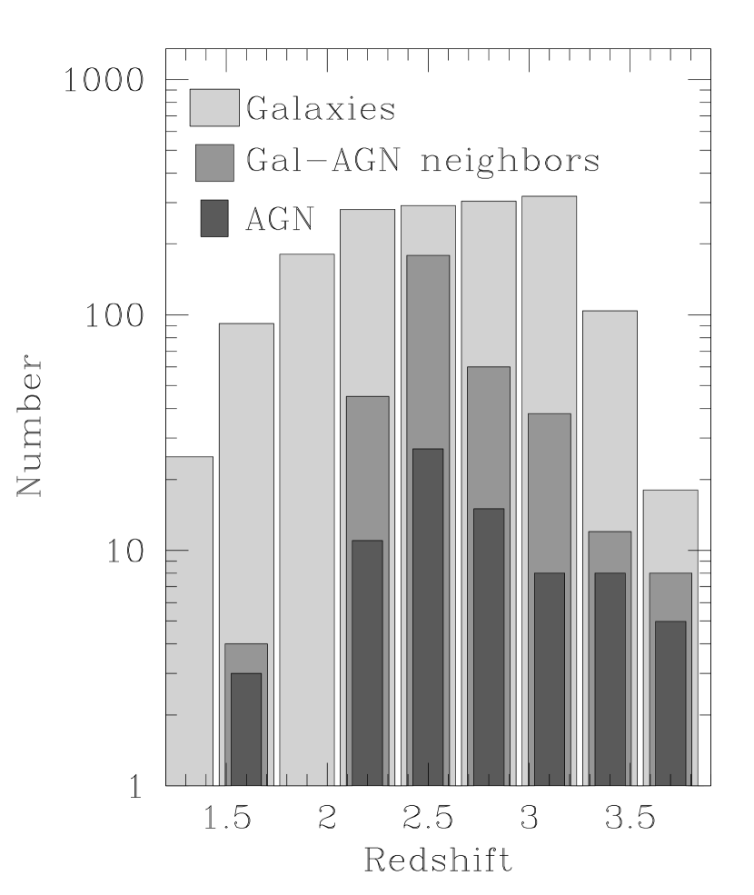
Figure 1.— Redshift distributions for the galaxies and AGN in our sample. Also shown is the number of galaxy-AGN neighbors, defined as the number of galaxy-AGN pairs with angular separation $60^{\prime\prime}<\theta<300^{\prime\prime}$ [$1.2\lower 2.15277pt\hbox{$\;\buildrel<\over{\sim}\;$}R/(h^{-1}{\rm comoving\,Mpc})\lower 2.15277pt\hbox{$\;\buildrel<\over{\sim}\;$}6.2$] and radial separation $\Delta Z<30h^{-1}$ comoving Mpc.

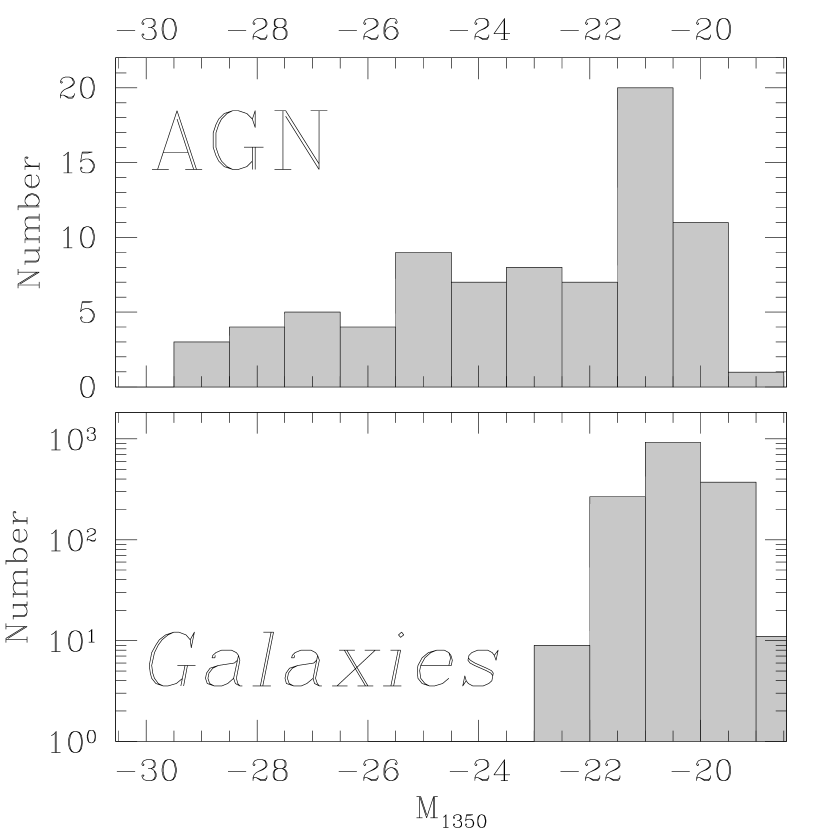
Figure 2.— Distribution of absolute AB magnitude at rest-frame $1350$Å for the AGN and galaxies in our spectroscopic sample. No corrections for incompleteness have been applied, so these do not resemble the true distributions for the underlying populations.

2.2. AGN

Fifty-seven of the 1684 objects in our spectroscopic sample have strong emission in both Lyman-$\alpha$ and CIV $\lambda 1549$. We classify these objects as AGN for reasons that are discussed in Steidel et al. (2002). Although some of our faintest AGN might be misclassified as galaxies because their CIV lines are too weak for us to detect, the lack of CIV emission in the thousand-object composite spectrum of Shapley et al. (2003) shows that these misclassified AGN must be rare.

Our total sample of AGN was increased to 79 by adding the previously known AGN that we deliberately included in our survey fields. Since CIV was the only line (aside from Lyman-$\alpha$) detected with reasonable significance in every AGN spectrum, we based our redshift assignments on it. In their analysis of 3814 QSOs from the Sloan Digital Sky Survey, Richards et al. (2002) found that CIV was blueshifted on average by 824 km s^-1 compared to MgII, which they assumed was at the QSO’s systemic redshift. We accordingly assumed that each of our AGN’s true redshift was 824 km s^-1 redder than the peak of CIV emission. Since Richards et al. (2002) report a scatter in the CIV–MgII velocity offsets of $500$ km s^-1, we expect that the uncertainty in our QSO redshifts will be approximately $500$ km s^-1. Although the way we assign redshifts is better suited to our sample’s broad-lined AGN, any mistakes in the redshifts of narrow-lined AGN are unlikely to affect our conclusions: as we will see, the typical redshift error would have to be $\sim 3000$ km s^-1 (i.e., $\sim 30h^{-1}$ comoving Mpc) to alter our clustering measurements significantly. Figure 1 shows the redshift distribution for the 79 AGN. Figure 3 shows their distribution of velocity FWHM and apparent magnitude.

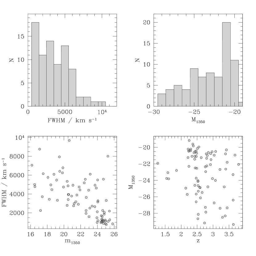
Figure 3.— Overview of the characteristics of the AGN in our sample. Upper left: Histogram of CIV line width. The typical uncertainty ranges from 10–20%, and is dominated by systematics (e.g., continuum placement) for the brightest AGN. Upper right: Histogram of absoluate AB magnitude at rest-frame 1350Å ($M_{1350}$). The uncertainty in the AB magnitude is $\lower 2.15277pt\hbox{$\;\buildrel<\over{\sim}\;$}0.2$ magnitudes for even our faintest objects (e.g., Steidel et al. 2003). Lower left: Relationship between CIV line width and apparent AB magnitude at rest-frame $1350$Å. Lower right: $M_{1350}$ against redshift. Recall that the selection bias is severe in our AGN sample, since (for example) we deliberately targeted AGN that were bright and had broad emission lines. These panels show the characteristics of our sample as selected, not of a fair sample of high-redshift AGN.

Strong emission lines prevented us from calculating the AGNs’ AB magnitudes at rest-frame 1350Å directly from their broadband magnitudes. Instead we scaled each AGN’s spectrum to match its observed $G$ and ${\cal R}$ magnitudes, measured the flux density near 1350Å, then converted to absolute magnitude for a cosmology with $\Omega_{M}=0.3$, $\Omega_{\Lambda}=0.7$, $h=0.7$. This procedure failed for our brightest sources, $G\lower 2.15277pt\hbox{$\;\buildrel<\over{\sim}\;$}18$, which were saturated in our images. For these we adopted the magnitude implied by their unscaled flux-calibrated spectra. Three of our sources were saturated and lacked flux-calibrated spectra. The magnitudes of these were taken from the Sloan Digital Sky Survey archive or from photographic measurements in the NASA/IPAC Extragalactic Database. Figure 2 shows the resulting histogram of AGN absolute magnitude. Although unintended, our selection strategy has given us a sample of AGN with brightnesses distributed almost uniformly over a 10-magnitude range. Comparison to the galaxies’ apparent magnitude distribution suggests that stellar light may contribute significantly to the measured magnitudes of the faintest AGN. We do not correct for this. Doing so would only strengthen our conclusions, since the faintest AGN would be even fainter than we assume.

2.3. Simulations

In a number of places our interpretation of the data relies on the GIF-LCDM numerical simulation of structure formation in a cosmology with $\Omega_{M}=0.3$, $\Omega_{\Lambda}=0.7$, $h=0.7$, $\Gamma=0.21$, and $\sigma_{8}=0.9$. This gravity-only simulation contained $256^{3}$ particles with mass $1.4\times 10^{10}h^{-1}M_{\odot}$ in a periodic cube of comoving side-length $141.3h^{-1}$ Mpc, used a softening length of $20h^{-1}$ comoving kpc, and was released publicly, along with its halo catalogs, by Frenk et al. astro-ph/0007362. Further details can be found in Jenkins et al. (1998) and Kauffmann et al. (1999). Although the simulation does not include much of the physics associated with galaxy formation, we make use only of its predictions for the statistical distribution of dark matter on large ($\;\buildrel>\over{\sim}\;$ Mpc) scales. Since the GIF-LCDM cosmology is consistent with the Wilkinson Microwave-Anisotropy Probe results (Spergel et al. 2003), and since modeling the gravitational growth of perturbations on large scales is not numerically challenging, the large-scale distribution of dark matter in this simulation should closely mirror that in the actual universe.

3. METHODS

3.1. Estimating $r_{0}$

We estimated the correlation lengths of the samples with two approaches. Both correct for the irregular angular sampling of our spectroscopy and are unaffected by the selection criteria that were used to include AGN in our sample. The second approach is also insensitive to the criteria that were used to select the galaxies. See Adelberger (2005) for a more complete discussion.

In the first approach, we cycle through the AGN in our sample, calculating for each one both the number $N_{\rm obs}(\ell)$ of galaxies in the AGN’s field whose comoving radial separation from the AGN, $\Delta Z$, is less than $\ell=30h^{-1}$ Mpc, and the number $N_{\rm exp}(\ell,r_{0})$ that would be expected if the correlation function had the form $\xi(r)=(r/r_{0})^{-1.6}$. The quantity $N_{\rm exp}(\ell,r_{0})$ is related straightforwardly to the integral of the correlation function along the lines of sight to galaxies in the field. As shown by Adelberger (2005),

$$N_{\rm exp}(\ell,r_{0})=\sum_{j}^{\rm galaxies}\frac{\int_{z_{i}-\Delta z}^{z_{i}+\Delta z}dz\,P_{j}(z)[1+\xi(r_{ij})]}{\int_{0}^{\infty}dz\,P_{j}(z)[1+\xi(r_{ij})]}$$ (1)

where the sum runs over all galaxies in the AGN’s field, $z_{i}$ is the AGN’s redshift, $\Delta z$ is the redshift difference corresponding to a comoving radial separation of size $\ell$, $P_{j}(z)$ is the selection function for the $j$th galaxy, normalized so that $\int_{0}^{\infty}dz\,P_{j}(z)=1$, and $r_{ij}$ is the distance between the AGN and a point at redshift $z$ with the galaxy’s angular separation $\theta_{j}$. We then sum the values $N_{\rm obs}(\ell)$ and $N_{\rm exp}(\ell,r_{0})$ for all our AGN, and take as our best-fit correlation length the value of $r_{0}$ that makes the total expected neighbor counts equal to the total observed. To ensure that our estimate of $r_{0}$ reflects the clustering strength on large ($\;\buildrel>\over{\sim}\;$ Mpc) scales, rather than conditions inside the AGNs’ halos, we exclude from consideration any galaxy-AGN pairs with angular separation $\theta<60^{\prime\prime}$ (i.e., $1.2h^{-1}$ comoving Mpc at $z=2.5$). Galaxy-AGN pairs with $\theta>300^{\prime\prime}$ are also excluded, since the weak clustering signal at the largest angular separations can be overwhelmed by low-level systematic errors (Adelberger 2005).

The approach of the preceding paragraph can fail if the assumed selection functions $P_{j}$ are inaccurate. To guard against this possibility, we also estimate $r_{0}$ by finding the value that makes

$$\frac{\sum_{\rm AGN}N_{\rm obs}(\ell)}{\sum_{\rm AGN}N_{\rm obs}(2\ell)}=\frac{\sum_{\rm AGN}N_{\rm exp}(\ell,r_{0})}{\sum_{\rm AGN}N_{\rm exp}(2\ell,r_{0})}$$ (2)

Taking the ratio causes most systematic errors to cancel (Adelberger 2005). Since it also increases the random errors, however, we use the equation 2 only to verify that systematic errors have not badly compromised the estimate of $r_{0}$ from the first approach.

3.2. Estimating the duty cycle

As stated in the introduction, our definition of duty cycle is the observed number density of AGN divided by the number density of halos that can host them. Calculating it requires two steps.

3.2.1 Halo abundance

We use the GIF-LCDM simulations to estimate the halo abundance from $r_{0}$. For each of the publicly released catalogs of halos at redshifts $2<z<3$, we calculated the cross-correlation function $\xi_{M_{1},M_{2}}(r)$ of halos in two mass ranges, $M>M_{1}$ and $M>M_{2}$, for different choices of $M_{1}$ and $M_{2}$, and estimated the cross-correlation length $r_{0}$ by fitting a power-law to $\xi_{M_{1},M_{2}}$ at separations $1<r/(h^{-1}{\rm Mpc})<10$. After calculating the number density of halos with $M>M_{2}$ in the simulations at redshift $z$, we stored our results as a table $r_{0}(z,M_{1},n_{2})$ giving the expected cross-correlation length at redshift $z$ between halos with mass threshold $M_{1}$ and halos with number density $n_{2}$. If all our observations were at redshift $z_{0}$ and we knew the threshold mass $M_{g}$ of the galaxies’ halos, we could convert any measured correlation length $r_{0}$ into a number density $n_{q}$ of AGN halos by simply looking up the value of $n_{q}$ that made the tabulated $r_{0}(z_{0},M_{g},n_{q})$ equal our observed correlation length. In fact our observations are at a range of redshifts and the galaxy mass is not precisely known. Figure 4 shows the uncertainty in the relationship between $r_{0}$ and $n_{q}$ that results from the range of redshifts in our survey and from the $1\sigma$ uncertainty in the galaxy masses (Adelberger et al. 2005a). For the remainder of the paper we will adopt an $r_{0}$–$n_{q}$ relationship that is a least-squares fit to the data in the figure (solid line). Although we can offer little justification for this compromise, the exact choice of relationship has almost no effect on our conclusions. Any errors in the relationship increase or decrease in tandem the implied duty cycles for bright and faint AGN; they alter the absolute value we infer for the duty cycles but not the relative difference between them. (We demonstrate that this is true in Figure 6, below.) This is one of the main strengths of our approach. It justifies our claim in § 1 that a systematic variation of AGN lifetime with luminosity is easier to measure than the absolute value of the lifetime itself.

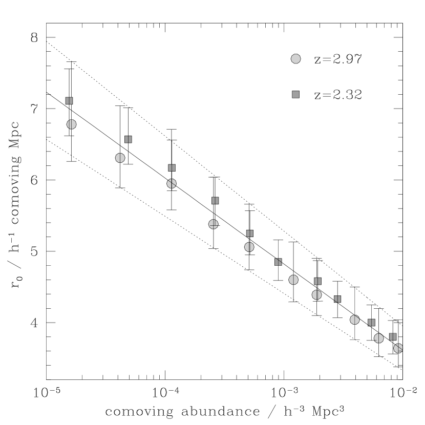
Figure 4.— Theoretical relationship between cross-correlation length $r_{0}$ and AGN-halo comoving abundance $n$. Points show the GIF-LCDM relationship at two redshifts. The error bars indicate the uncertainty in the relationship due to the uncertainty in the galaxies’ threshold mass. The solid line shows the least-squares compromise that we adopt throughout: $\log(n/(h^{-1}{\rm Mpc})^{3})=-0.83r_{0}+1.00$. The upper and lower dotted lines show the relationships that would result if we altered the assumed threshold mass by $\pm 1\sigma$. Figure 6 shows that our conclusions would not be significantly affected if we adopted these relationships instead.

3.2.2 AGN abundance

We adopt a crude approach since small (tens of percent) errors in the AGN abundance have little effect on our conclusions. At the faintest magnitudes we estimate the AGN number density by multiplying the galaxy luminosity function at $z=3$ (Adelberger & Steidel 2000) by $f(M_{1350})$, the fraction of sources in our spectroscopic sample with absolute magnitude $M_{1350}$ that were observed to be AGN. Note that we are including all AGN in this analysis, not merely the broad-lined AGN considered by Hunt et al. (2004). Since the faint end of the rest-frame UV luminosity distribution of galaxies does not evolve significantly from $z=3$ to $z=2$ (N.A. Reddy et al. 2005, in preparation), this number density should be roughly appropriate down to $z=2$. At the brightest magnitudes we adopt the “2dF” $1.81<z<2.10$ QSO luminosity function of Croom et al. (2004). The AGN luminosity distribution is fit tolerably well by a Schechter function (figure 5), and we use this fit to estimate the number density of AGN in each range of apparent magnitude.

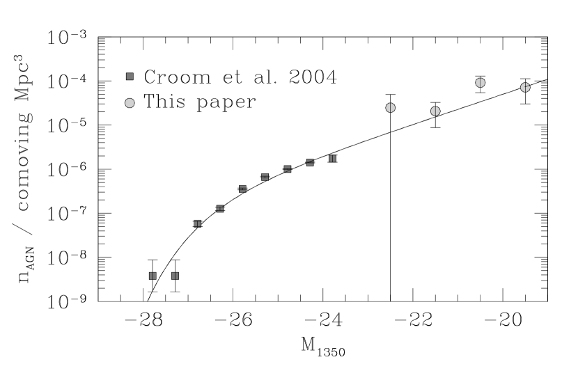
Figure 5.— Observed number density vs. magnitude for AGN at $z\sim 2$. Squares show the 2dF QSO luminosity function of Croom et al. (2004). Circles show our rough estimate of the AGN luminosity function at fainter magnitudes, calculated from our survey with the method described in § 3.2.2. The crude completeness corrections of this approach yield a luminosity function adequate only for cases like ours where low accuracy is tolerable. The parameters of the Schechter-function (solid line; $M_{\ast}=-26.2$, $\alpha=-1.85$, $\Phi_{\ast}=4\times 10^{-7}$ Mpc^-3) should not be used in other situations.

4. RESULTS

The first approach of § 3.1 leads to the estimates $r_{0}=4.7,5.4$ comoving Mpc for the galaxy-AGN cross-correlation length of AGN with magnitude $-30<M_{1350}<-25$ and $-25<M_{1350}<-19$, respectively. An easy way to estimate the uncertainty is suggested by the similarity of the cross-correlation length to the galaxy-galaxy correlation length reported by Adelberger et al. (2005a): generate many alternate realizations of the data by treating randomly chosen galaxies in each field as that field’s AGN, rather than the true AGN themselves, and recalculate $r_{0}$ for each simulated sample. The rms dispersion of $r_{0}$ among these simulated samples should be roughly equal to the uncertainty in $r_{0}$, and we adopted it for the error bars in the top panel of Figure 6. The true uncertainty is likely to be somewhat smaller, since our spectroscopic selection strategy gave our AGN more angular neighbors with measured redshifts than the typical galaxy.

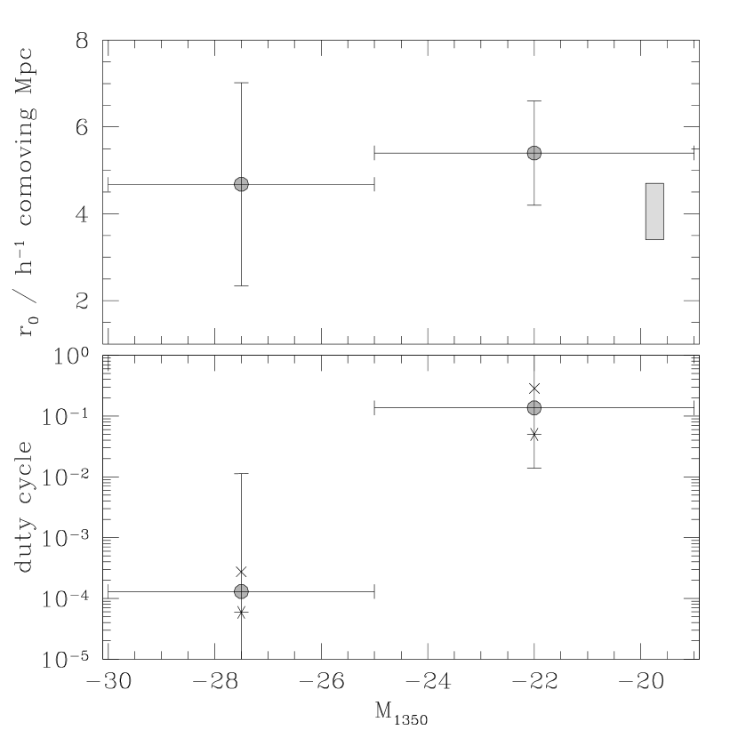
Figure 6.— Top panel: galaxy-AGN cross-correlation length as a function of AGN luminosity $M_{1350}$. Points with error bars show our measurements. The shaded square shows the $\pm 1\sigma$ range of the galaxy-galaxy correlation length at similar redshifts (Adelberger et al. 2005a); its abscissa is arbitrary. Bottom panel: implied duty cycle as a function of AGN luminosity. Error bars show the $\pm 1\sigma$ random uncertainty. The four- and six-pointed stars show how our estimated duty cycle would change if we altered the assumed relationship between clustering strength and abundance by an amount similar to its uncertainty. (They correspond to the upper and lower dotted envelopes in Figure 4.) Note that the confidence intervals shown in this plot reflect only the constraints from our clustering analysis. Other considerations rule out a duty cycle of $\lower 2.15277pt\hbox{$\;\buildrel>\over{\sim}\;$}1$ for the faint AGN and $\lower 2.15277pt\hbox{$\;\buildrel<\over{\sim}\;$}10^{-5}$ for the bright AGN, however. See § 5 for further discussion.

The bottom panel of Figure 6 shows the same data, except the cross-correlation length has been converted to a duty cycle with the approach of § 3.2. As emphasized in that section, uncertainties in the $r_{0}$–abundance relationship mean that the labels on the $y$ axis could be wrong by a multiplicative constant, but relative differences in duty cycle should be secure.

To estimate the significance of the apparent difference in duty cycle, we note that our adopted relationship between $r_{0}$ and halo number density implies that $r_{0}$ would be $2.92h^{-1}$ comoving Mpc larger for AGN with $-30<M_{1350}<-25$ than AGN with $-25<M_{1350}<-19$ under the null hypothesis that the duty cycle is independent of $M_{1350}$. The observed difference in best-fit correlation length, $-0.72h^{-1}$ comoving Mpc, is therefore $3.64h^{-1}$ comoving Mpc smaller than the difference that would be expected under the null hypothesis. A difference as large or larger than $\Delta r_{0}=3.64h^{-1}$ Mpc between AGN with $-25<M_{1350}<-19$ and $-30<M_{1350}<-25$ occurred in 10% of the randomized AGN samples described above. We conclude that the null hypothesis of a constant duty cycle can be rejected with roughly 90% confidence.

5. SUMMARY & DISCUSSION

We measured the galaxy-AGN cross-correlation length $r_{0}$ as a function of AGN luminosity. The cross-correlation length was similar for bright and faint AGN, $r_{0}=4.7\pm 2.3$ for $-30<M_{1350}<-25$ and $r_{0}=5.4\pm 1.2$ for $-25<M_{1350}<-19$, which led us to conclude with $90$% confidence that both are found in halos with similar masses and that bright AGN are rarer because their duty cycle is shorter. Since halo lifetimes depend only weakly on halo mass (e.g., Martini & Weinberg 2001), the difference in duty cycle implies that optically faint AGN have longer lifetimes.

Our analysis differs from previous work (e.g., that of Croom et al. 2005, who also found no luminosity dependence in the AGN clustering strength) in two principal ways. We estimated the duty cycle from the cross-correlation of galaxies and AGN, not from the auto-correlation function of AGN, and our sample included AGN with a much wider range of luminosities, extending $\sim 4$ magnitudes fainter than the QSO threshold $M_{1350}=-23$. These differences allowed us to obtain our measurement from a comparatively small survey.

An appraisal of this result should cover at least the following three points.

The first is obvious: it is only marginally significant. Larger samples will be required to prove that the duty cycle depends on luminosity. Moreover, other arguments suggest that the minimum allowed duty cycle at high luminosity should be increased and the maximum allowed at low luminosity should be decreased. Since the AGN lifetime is roughly the age of the universe times the duty cycle (e.g., Martini & Weinberg 2001), a duty cycle of $\lower 2.15277pt\hbox{$\;\buildrel<\over{\sim}\;$}10^{-5}$ for the brightest AGN is incompatible with the observed proximity effect in QSOs’ spectra (e.g., Martini 2004) and with the lack of flickering QSOs in the Sloan Digital Sky Survey (Martini & Schneider 2003). A duty cycle of roughly unity for the fainter AGN is implausible as well, since a black hole radiating continuously would almost certainly be too faint compared to its galaxy for us to detect: the difference in energetic efficiency for black hole accretion ($0.1mc^{2}$) and hydrogen burning ($0.007mc^{2}$) implies that a galaxy’s steadily radiating black hole would be much fainter than its stars if the final ratio of black hole to stellar mass is $M_{\rm BH}/M_{\ast}\sim 0.001$. Taking these arguments into account would bring the high and low luminosity duty cycles closer together in Figure 6.

Second, the physical interpretation is not straightforward. Recall that we have defined the duty cycle for the absolute magnitude range $M_{\rm lo}<M<M_{\rm hi}$ as the ratio of the number density of AGN with those magnitudes to the number density of halos that can host them. In the appendix we show that this duty cycle would be independent of magnitude if blackholes accreted only at the Eddington rate, were not obscured by dust, and had masses that followed a tight power-law correlation with the total masses $M_{h}$ of galaxies that contain them. The duty cycle would decrease at large luminosities if brighter AGN were more heavily obscured, if black hole masses fell below the predictions of the $M_{\rm BH}$–$M_{h}$ correlation at very large $M_{h}$, or if anything (e.g., complicated light curves) gave a broad range of luminosities $L$ to the AGN that lie within halos of a given mass $M_{h}$. Each of these is expected theoretically (e.g., Hopkins et al. 2005). The apparent decrease of duty cycle at large luminosities presumably results from a combination of physical effects, and our observations do not identify which is dominant among them.

Finally, our result was derived from a small survey designed for other purposes. Most of the brightest AGN lay behind the survey galaxies, not in their midst, reducing the number of galaxy-AGN pairs and increasing the uncertainty in $r_{0}$. A large, optimized survey could easily shrink the error bars several fold. The only useful contribution of this paper may be its demonstration that a definitive measurement is within easy reach.

KLA would like to thank L. Ho, L. Hernquist, L. Ferrarese, and J. Kollmeier for many interesting conversations and an anonymous referee for encouraging us to discuss the physical interpretation of the duty-cycle. Our collaborators in the Lyman-break survey did most of the work in taking and reducing these data. We are grateful that they let us proceed with the analysis. This research has made use of the NASA/IPAC Extragalactic Database (NED) which is operated by the Jet Propulsion Laboratory, California Institute of Technology, under contract with the National Aeronautics and Space Administration.

Appendix A PHYSICAL INTERPRETATION OF THE DUTY CYCLE

We discuss three simple models for AGN evolution that may help illustrate the physical meaning of the duty cycle.

Suppose first that black hole mass $M_{\rm BH}$ is tightly correlated with total galaxy mass $M_{h}$ at all times, that the correlation has the form $M_{\rm BH}\propto M_{h}^{\alpha}$, that AGN are unobscured by dust, and that black holes radiate either at the Eddington rate $L_{\rm Edd}(M_{\rm BH})$ or not at all, gaining their mass in a few short accretion episodes separated by long periods of quiescence. The duty cycle would then be independent of AGN magnitude, as can be seen with the following argument.

Begin by considering the evolution of a black hole inside a single dark matter halo of given mass $M_{h}$. When the halo forms in the very early stages of a merger of two smaller halos, its black hole mass may initially be smaller than the mean mass implied by the $M_{\rm BH}$–$M_{h}$ correlation, but by the time the halo is destroyed by mergers, roughly one Hubble time later (Martini & Weinberg 2001), the black hole must have grown enough to fall on the correlation. Otherwise the correlation could not be satisfied by the ensemble of all halos. Since accretion at the Eddington rate produces exponential growth, the black hole will spend equal amounts of time in each octave of luminosity as it grows from its initial mass $M_{i}$ to its final mass $M_{f}$; if one were to plot the amount of time spent in each logarithmic interval of luminosity $L$, it would be constant for $L_{\rm Edd}(M_{i})<L<L_{\rm Edd}(M_{f})$ and 0 elsewhere. This is equally true if the growth occurs in many discrete episodes of accretion or in a single burst. Now consider a plot of total elapsed time versus luminosity for the black holes within $N$ randomly chosen halos of the same mass $M_{h}$. It would be the superposition of $N$ boxcars with random left and right edges, producing an overall shape that is peaked near the Eddington luminosity of the typical black hole associated with halos of mass $M_{h}$. Figure 7 shows an example for $N=6$. The same plot for the ensemble of all halos of mass $M_{h}$ would be a smoother realization of a similar function. Call this plot the kernel. Since the number of AGN we observe with a given luminosity is proportional to the net time AGN spend at that luminosity, the kernel is the AGN luminosity distribution we would observe if the universe consisted solely of halos with mass $M_{h}$. The width of the kernel depends on how far the initial and final black hole masses stray from the expectation value $E(M_{\rm BH}|M_{h})$, but it must be very narrow compared to the multi-decade width of the halo mass distribution. Otherwise our assumption of a tight $M_{\rm BH}$–$M_{h}$ correlation would be violated. The AGN within a narrow range of luminosity therefore must lie inside halos with a narrow range of masses. Our definition of duty cycle for $L_{\rm min}<L<L_{\rm max}$ is the number density of AGN within that range of luminosity divided by the number density of halos that can host them. In this scenario, it is equal to the time required for the AGN’s luminosity to grow from $L_{\rm min}$ to $L_{\rm max}$ if it is accreting at the Eddington rate divided by the halos’ mean lifetime. The numerator is independent of halo mass for logarithmic luminosity intervals, and the denominator depends extremely weakly on halo mass (Martini & Weinberg 2001). Therefore the duty cycle in logarithmic luminosity bins should be nearly independent of halo mass or AGN luminosity.

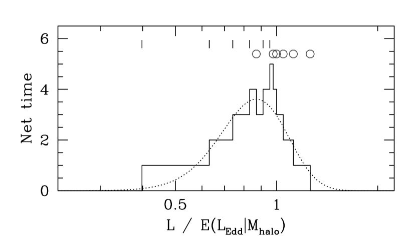
Figure 7.— Net time spent at a given luminosity for an ensemble of 6 blackholes in the first toy model considered in the appendix. We assume that these black holes radiate at the Eddington luminosity and lie inside 6 halos of equal mass $M_{h}$. If the blackholes have the initial luminosities that are marked with vertical lines, and they grow until the luminosities have reached the final values marked with circles, then the total amount of time the 6 AGN spent radiating at a given luminosity is shown by the solid histogram. The distribution for all AGN in halos of mass $M_{h}$, not just these 6 AGN, might look more like the dotted curve in the background. If black hole and halo mass are tightly correlated and all accretion is at the Eddington rate, this function has to be narrow. The units on the $x$ axis are normalized to $E(L_{\rm Edd}|M_{h})$, the mean Eddington luminosity of all AGN in halos of mass $M_{h}$; units on the $y$ axis are arbitrary.

To check this claim, we generated an ensemble of simulated AGN by starting with an ensemble of halos following a Press-Schechter mass function ($\Omega_{M}=0.3$, $\Omega_{\Lambda}=0.7$, $\Gamma=0.2$, $\sigma_{8}=0.9$, $z=2.5$), assigning each halo an expected central blackhole mass with the relationship $M_{\rm BH}=10^{7}(M_{h}/10^{12}M_{\odot})^{1.65}$ (Ferrarese 2002), and giving each black hole a luminosity equal to the Eddington luminosity of the expected mass times a random number drawn at random from the kernel (Figure 7). This resulted in the AGN luminosity distribution shown in the upper left panel of Figure 8. The distribution of halo masses for AGN with luminosities $L_{\rm Edd}(10^{6}M_{\odot})<L<L_{\rm Edd}(10^{8}M_{\odot})$ and $L_{\rm Edd}(10^{8}M_{\odot})<L<L_{\rm Edd}(10^{10}M_{\odot})$ is shown in the middle left panel. The bottom panel shows the inferred duty cycle in these luminosity ranges, i.e., the ratio of AGN number density in each luminosity range to the number density of halos more massive than the mean associated halo mass shown in the middle left panel. This is roughly the duty cycle that would be estimated with the approach we adopted above. It is the same for the two logarithmic luminosity ranges, as expected.

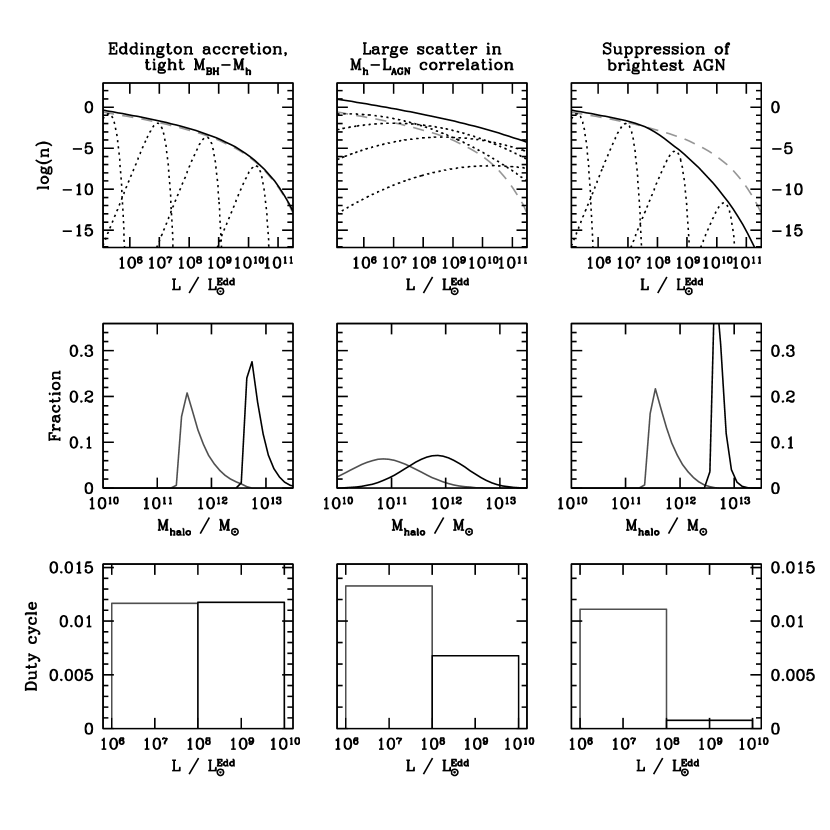
Figure 8.— Dependence of duty cycle on luminosity for three toy models. We generated an ensemble of simulated central black holes from a Press-Schechter mass function by associating each halo of mass $M_{h}$ with a blackhole of expected mass $M_{\rm BH}/M_{\odot}=10^{7}(M_{h}/10^{12}M_{\odot})^{1.65}$ (Ferrarese 2002), then associated each blackhole with a luminosity under different assumptions for the three models. Each column shows results for one model. Left panels assume Eddington accretion and a tight correlation of $M_{h}$ and $M_{\rm BH}$. Middle panels assume large scatter in the relationship between $M_{h}$ and AGN luminosity $L$. Right panels assume Eddington accretion but stunt the growth of blackholes in the most massive halos. Units on the $y$ axis are arbitrary in all panels. Top panels: Dashed lines show the luminosity distribution that would have resulted if each black hole had exactly the mean mass predicted by the $M_{\rm BH}$–$M_{h}$ relationship and radiated at its Eddington luminosity. Instead we assumed that each halo’s AGN luminosity had some scatter around its expectation value. Dotted lines indicate the assumed luminosity distribution for halos of mass $10^{12},10^{13},10^{14},10^{15}M_{\odot}$. They show the assumed scatter in the $M_{h}$–$L$ relationship, which is large for the middle model and equally small for the left and right models. The solid lines show the implied AGN luminosity function. (More-realistic models would keep the AGN luminosity function fixed to the observations by adjusting other parameters, but these simple models are sufficient to illustrate our point.) Middle panels: Distribution of mass for halos that host AGN with luminosities $10^{6}L^{\rm Edd}_{\odot}<L<10^{8}L^{\rm Edd}_{\odot}$ and $10^{8}L^{\rm Edd}_{\odot}<L<10^{10}L^{\rm Edd}_{\odot}$. Here $L^{\rm Edd}_{\odot}$ is the Eddington luminosity of a solar-mass blackhole. Bottom panels: Derived duty cycle for AGN in the same luminosity ranges. The duty cycles were estimated by dividing the number of AGN in the luminosity range by the number density of halos more massive than the mean shown in the middle panels. These panels show that the duty cycle will decrease at high luminosities if there is significant scatter in the $M_{h}$–$L$ relationship or if black hole accretion is suppressed in the most massive halos. Increases in dust obscuration with luminosity can also reduce the duty cycle at high $L$, but we judged this effect too obvious to illustrate here.

The scenario can be altered in two ways to make the duty cycle decrease at larger luminosities.

The first is to increase the number density of halos that can host the brightest AGN. For a fixed halo mass distribution, this can be accomplished by relaxing our assumption that accretion occurs only at the Eddington rate or by increasing the scatter in the $M_{\rm BH}$–$M_{h}$ relationship. Either increases the scatter in the relationship between $M_{h}$ and $L$, raising the probability that a high luminosity AGN resides within a low mass halo. The middle column of Figure 8 shows one example of how a broad distribution of $L$ at fixed $M_{h}$ makes the duty cycle depend on luminosity.

The second way is to reduce the lifetimes of the brightest AGN. If the $M_{\rm BH}$–$M_{h}$ correlation is a tight power-law and all accretion is at the Eddington rate, then we can adjust neither the mean accreted mass for blackholes in the most massive halos nor the rate at which accretion occurs. In this case lifetimes of the brightest AGN can be reduced only by making them heavily obscured while they accrete most of their mass. The lifetimes can also be reduced, even for unobscured Eddington-rate accretion, if we change the form of the $M_{\rm BH}$–$M_{h}$ relationship. One change seems well motivated: letting it break down for halos with super-galactic masses. Ferrarese’s (2002) relationship $M_{\rm BH}\sim 10^{7}(M_{h}/10^{12}M_{\odot})^{1.65}M_{\odot}$ predicts that local clusters of mass $10^{15}M_{\odot}$ should contain $10^{12}M_{\odot}$ central blackholes, for example, but there is no evidence that these ultra-massive blackhole exist. It seems more likely that blackhole formation becomes as suppressed as star-formation in halos with mass $M_{h}\gg 10^{13}M_{\odot}$. Suppressing or obscuring the brightest AGN can make the duty cycle depend strongly on luminosity, as Figure 8 shows.

If additional observations confirm the decrease in duty cycle at high luminosities, some combination of these effects would presumably be responsible.

References

- (1) Adelberger, K.L., Steidel, C.C., Giavalisco, M., Dickinson, M., Pettini, M. & Kellogg, M. 1998, ApJ, 505, 18
- (2) Adelberger, K.L. & Steidel, C.C. 2000, ApJ, 544, 218
- (3) Adelberger, K.L., Steidel, C.C., Shapley, A.E., Hunt, M.P., Erb, D.K., Reddy, N.A., & Pettini, M. 2004, ApJ, 607, 226
- (4) Adelberger, K.L., Steidel, C.C., Pettini, M., Shapley, A.E., Reddy, N.A., & Erb, D.K. 2005a, ApJ, 619, 697
- (5) Adelberger, K.L. 2005, ApJ, 621, 574
- (6) Adelberger, K.L. et al. 2005b, ApJ, in press (astro-ph/0505122)
- (7) Cristiani, S. & Vio, R. 1990, A& A, 227, 385
- (8) Croom, S.M., Smith, R.J., Boyle, B.J., Shanks, T., Miller, L., Outram, P.J., & Loaring, N.S. 2004, MNRAS, 349, 1397
- (9) Croom, S.M., Boyle, B.J., Shanks, T., Smith, R.J., Miller, L., Outram, P.J., Loaring, N.S., Hoyle, F., & da Ângela, J. 2005, MNRAS, 356, 415
- (10) Ferrarese, L. 2002, ApJ, 578, 90
- (11) Haiman, Z. & Hui, L. 2001, ApJ, 547, 27
- (12) Ho, L. 2004, in “Carnegie Observatories Astrophysics Series, Vol I”, ed. L. Ho (Cambridge: Cambridge Univ. Press), p292
- (13) Hopkins, P.F., Hernquist, L., Cox, T.J., Di Matteo, T., Martini, P., Robertson, B., & Springel, V. 2005, ApJ, submitted (astro-ph/0504190)
- (14) Hunt, M.P., Steidel, C.C., Adelberger, K.L., & Shapley, A.E. 2004, ApJ, 605, 625
- (15) Jenkins, A., Frenk, C.S., Pearce, F.R., Thomas, P.A., Colberg, J.M., White, S.D.M., Couchman, H.M.P., Peacock, J.A., Efstathiou, G., & Nelson, A.H., 1998, ApJ, 499, 20
- (16) Kaiser, N. 1984, ApJ, 284, L9
- (17) Kauffmann, G., Colberg, J.M., Diafero, A., & White, S.D.M., 1999, MNRAS, 303, 188
- (18) Kauffmann, G. & Haehnelt, M.G. 2002, MNRAS, 332, 529
- (19) Lynden-Bell, D. 1969, Nature, 223, 690
- (20) Martini, P. 2004, in “Carnegie Observatories Astrophysics Series, Vol I”, ed. L. Ho (Cambridge: Cambridge Univ. Press), p170
- (21) Martini, P. & Schneider, P. 2003, ApJ, 597, L109
- (22) Martini, P. & Weinberg, D.H. 2001, ApJ, 547, 12
- (23) Merloni, A. 2004, MNRAS, 353, 1035
- (24) Richards, G.T., Vanden Berk, D.E., Reichard, T.A., Hall, P.B., Schneider, D.P., SubbaRao, M., Thakar, A.R., & York, D.G., 2002, AJ, 124, 1
- (25) Shapley, A.E., Steidel, C.C., Pettini, M., & Adelberger, K.L. 2003, ApJ, 588, 65
- (26) Soltan, A. 1982, MNRAS, 200, 115
- (27) Spergel, D.N. et al. 2003, ApJS, 148, 175
- (28) Steidel, C.C., Hunt, M.P., Shapley, A.E., Adelberger, K.L., Pettini, M., Dickinson, M., & Giavalisco, M. 2002, ApJ, 576, 653
- (29) Steidel, C.C., Adelberger, K.L., Shapley, A.E., Pettini, M., Dickinson, M., & Giavalisco, M. 2003, ApJ, 592, 728
- (30) Steidel, C.C., Shapley, A.E., Pettini, M., Adelberger, K.L., Erb, D.K., Reddy, N.A., & Hunt, M.P. 2004, ApJ, 604, 534