STEllar Content from high resolution galactic spectra
via Maximum A Posteriori

Abstract

This paper describes STECMAP (STEllar Content via Maximum A Posteriori), a flexible, non-parametric inversion method for the interpretation of the integrated light spectra of galaxies, based on synthetic spectra of single stellar populations (SSPs). We focus on the recovery of a galaxy’s star formation history and stellar age-metallicity relation. We use the high resolution SSPs produced by Pégase-HR to quantify the informational content of the wavelength range $\lambda\lambda=4000-6800$ Å. Regularization of the inversion is achieved by requiring that the solutions are relatively smooth functions of age. The smoothness parameter is set automatically via generalized cross validation.

A detailed investigation of the properties of the corresponding simplified linear problem is performed using singular value decomposition. It turns out to be a powerful tool for explaining and predicting the behaviour of the inversion, and may help designing SSP models in the future. We provide means of quantifying the fundamental limitations of the problem considering the intrinsic properties of the single stellar populations in the spectral range of interest, as well as the noise in these models and in the data. We demonstrate that the information relative to the stellar content is relatively evenly distributed within the optical spectrum. We show that one should not attempt to recover more than about 8 characteristic episodes in the star formation history from the wavelength domain we consider. STECMAP preserves optimal (in the cross validation sense) freedom in the characterization of these episodes for each spectrum.

We performed a systematic simulation campaign and found that, when the time elapsed between two bursts of star formation is larger than 0.8 dex, the properties of each episode can be constrained with a precision of 0.04 dex in age and 0.02 dex in metallicity from high quality data ($R=10\,000$, signal-to-noise ratio $\mathrm{SNR}=100$ per pixel), not taking model errors into account. We also found that the spectral resolution has little effect on population separation provided low and high resolution experiments are performed with the same SNR per Å. However, higher spectral resolution does improve the accuracy of metallicity and age estimates in double burst separation experiments. When the fluxes of the data are properly calibrated, extinction can be estimated; otherwise the continuum can be discarded or used to estimate flux correction factors.

The described methods and error estimates will be useful in the design and in the analysis of extragalactic spectroscopic surveys.

1 Introduction

The diversity of shapes and colors of galaxies illustrates the wealth of physical mechanisms acting in these complex objects. Their formation history, including the building of their halos, bulges, disks and disk patterns, is still controversial. Empirical constraints on the formation scenarii are engraved in the distribution of stellar ages, metallicities, and kinematics. Unless the galaxies can be resolved into stars, this crucial information must be extracted from integrated spectra. This spectral energy distribution is a recording of the whole life of a galaxy: the condition of its birth, the formation and assembly of its first blocks, its passive evolution and the recycling of its material, or its active evolution through merging, all these determine the current stellar content. Yet, this information is embedded in a non-trivial manner in the light we receive.

While a wealth of such data is currently being gathered from spectroscopic surveys (for example the Sloan Digital Sky Survey or the 2DF Galaxy Redshift Survey), using them to probe the general properties of the stellar populations on a cosmological timescale is an exciting perspective.

In the literature, the stellar content of a galaxy is often characterized by a luminosity weighted age, a luminosity weighted metallicity, a global velocity dispersion, and a parameter characterizing extinction. Since Worthey (1994), the Lick indices have been readily used in order to describe the nature of the stellar populations. Spectral indices are convenient because they are robust to a number of observational perturbations, but they exploit only small wavelength domains. The use of a larger fraction, and eventually of all the information in a spectrum must, at least in principle, help separate, age-date and characterize coexisting stellar components, steps required to access the actual evolution of the galaxies under study. Individual spectral features with specific sensitivities to age or metallicity may add information to the Lick data points, and the redundancy provided by many lines spread over a wide spectral range reduces the sensitivity to noise. Recently, methods have emerged that use the whole available spectral range, relying on compression (Reichardt et al., 2001) or on non-negative least squares (Mateu et al., 2001; Cid Fernandes et al., 2004).

The introduction of these methods gave birth to a field of research, whose goal is to measure the cosmic star formation history by summing the individual star formation histories of a large number of galaxies. This results in an estimate of the mean history of star formation (a so called “Madau plot”) in principle free from the uncertainties related to pure emission-line diagnostics (Dopita, 2005). Moreover, the distribution of individual star formation histories is even more constraining than a Madau plot alone. If feasible, this approach indeed constitutes a very powerful test for the current cosmological models. In fact, such techniques have been used recently to support the idea of galactic downsizing, i.e. to argue the stellar activity has shifted in the recent past towards less massive galaxies, something that some authors have presented as a problem for hierarchical clustering. As more results of this kind are published, it becomes clear that different authors have very different conceptions of what is a reasonable interpretation of a galactic spectrum (Cid Fernandes et al., 2004; Heavens et al., 2004). Indeed, the problem of characterizing star formation histories based on a spectrum is strongly ill-conditioned as we will demonstrate extensively below (see also Moultaka & Pelat 2000; Moultaka et al. 2004). This remains true in the restrictive framework of evolutionary population synthesis, although this approach incorporates the simplifying assumption that the intrinsic spectra of mono-metallic, single-aged single stellar populations (SSPs) are known. Over-interpretation of the data is a common pitfall when ill-conditioning is misjudged or overlooked. A useful approach to ill-conditioned inverse problems is the maximum penalized likelihood, which is formally equivalent to a maximum a posteriori likelihood (MAP). It has been applied in the past in a variety of fields in astronomy such as light deprojection (Kochanek & Rybicki, 1996), stellar kinematics (Saha & Williams, 1994; Merritt, 1997; Pichon & Thiébaut, 1998), image deblurring (Thiébaut, 2002, 2005) or the interpretation of low resolution energy distributions of galaxies (Vergely et al., 2002).

This paper discusses the interpretation of high resolution optical spectra of galaxies. A maximum resolving power $R=10\,000$ is considered, which is adequate in particular for the studies of low mass galaxies or of massive star clusters in galaxy cores. We focus on the object’s stellar content. The simultaneous extraction of the kinematical information with a direct extension of the adopted method is the subject of a companion paper. Our work is positioned at the interface between single stellar population models and observations. Its purpose is not to question the particular ingredients and assumptions of a specific population synthesis code, although some of the discussion will be specific to the model package Pégase-HR of Le Borgne et al. (2004), since it is the first package to have provided a similar spectral resolution (see Gonzalez Delgado et al. (2005) for a medium resolution package). Rather, we intend to clarify how the intrinsic properties of a basis of single stellar population spectra can be used to infer consequences for the study of composite stellar populations.

The general problem, where additional constraints such as positivity of the star formation history are included is a non-linear problem. Nevertheless, we give special importance to the linear problem because it provides firm footing to explain the processes that determine the reliability of a recovered star formation history. It also clearly displays many of the features found in the more realistic inversions as well.

We also study the feasibility of the inversion in different observational regimes (in terms of spectral resolution and noise), and give simple scaling laws and error estimates to predict the accuracy and relevance of the results. The main characteristics of our approach are:

• It is non parametric, and thus provides properties such as the stellar age distribution with minimal constraints on their shape.

• The ill-conditioning of the problem is taken into account through explicit regularization.

• Optimal interpretation of the data is achieved by the proper setting of the smoothing parameter.

The organization of the paper is as follows. We start in Sect. 2 by describing the inversion problems that will be tackled. In Sect. 3, we provide a comprehensive investigation of the idealized linear problem of finding the stellar age distribution of a mono-metallic, reddening-free stellar population. Sect. 4 investigates the performance of these inversions in a set of simulations in terms of resolution and separability of bursts. Sect. 5 addresses the problem of the simultaneous study of stellar ages and metallicities, while allowing for extinction (or other transformations of the continuum). Conclusions are drawn in Sect. 6, while the paper closes with a discussion for prospects.

2 Non parametric models of spectra

The spectral energy distribution (SED) that we measure for each spatial pixel of an observed galaxy results from light emitted by coexisting stellar populations of various ages, metallicities and kinematics, and from the interactions of the stellar light with the interstellar medium (reddening, nebular emission). The example of the Milky Way tells us that any given stellar population of a galaxy may consist of stars with non-trivial distributions in age, metallicity, or even relative abundances (Feltzing et al., 2001; Prochaska et al., 2000; Gratton et al., 2000). In principle, age, abundances and velocity distributions should thus be treated as independent parameters in a galaxy model meant for an exploration without preconceptions.

In the following, we will restrict ourselves to simplified models that balance, in our view, technical feasibility (in view of current models and data) and scientific interest. We assume that metallicity describes the stellar abundances, mainly because our population synthesis model does not allow for abundance variations (Thomas et al. (2003) specifically address this issue). Except for the discussion of a more general case in Sect. 5, we restrict ourselves to the assumption of a one to one relationship between stellar ages and metallicities. This allows us to search for significant trends, as predicted by simple evolutionary scenarii for galaxies. We adopt a simple parameterized formulation for extinction. Finally, we will deal with stellar populations at rest (or with known velocity distributions).

Emission lines are out of the aim of this study. They may be used in the future, in particular to obtain further constraints on the youngest stars and on obscuration by dust, or to constrain properties of the interstellar medium.

2.1 The spectral basis

The basic building block to model the spectrum of an observed galaxy is the spectral energy distribution $S(\lambda,m,t,Z)$ of a star of initial mass $m$, age $t$ and metallicity $Z$ (mass fraction of metals at the formation of the star). Integrating over stellar masses yields the intrinsic spectrum $B^{0}(\lambda,t,Z)$ of the single stellar population of age $t$, metallicity $Z$ and unit mass:

$$B^{0}(\lambda,t,Z)\triangleq\int_{{M_{\mathrm{min}}}}^{{M_{\mathrm{max}}}}\operatorname{IMF}(m)\,S(\lambda,m,t,Z)\,\mathrm{d}m\,,$$ (1)

where $\operatorname{IMF}(M)$ is the Initial Mass Function and ${M_{\mathrm{min}}}$ and ${M_{\mathrm{max}}}$ are the lower and upper mass cut-offs of this distribution. Assuming that the metallicities of the stars can be described by a single-valued Age-Metallicity Relation (AMR) $Z(t)$, it is possible to derive the unobscured spectral energy distribution of the galaxy at rest:

$$F_{\mathrm{rest}}(\lambda)=\int_{{t_{\mathrm{min}}}}^{{t_{\mathrm{max}}}}\operatorname{SFR}(t)\,B^{0}(\lambda,t,Z(t))\,\mathrm{d}t\,,$$ (2)

where $\operatorname{SFR}(t)$ is the Star Formation Rate (i.e. mass of new stars born per unit of time, with the convention that $t=0$ is today) and ${t_{\mathrm{max}}}$ is an upper integration limit, for instance the Hubble time. Similarly, ${t_{\mathrm{min}}}$ is a lower integration limit, ideally 0. Both ${t_{\mathrm{min}}}$ and ${t_{\mathrm{max}}}$ must in practice be set according to the validity domain of the SSP basis $B^{0}(\lambda,t,Z(t))$.

The Luminosity Weighted Stellar Age Distribution (LWSAD) $\Lambda(t)$ gives the contribution to the total emitted light of stars of age $[t,t+\mathrm{d}t]$. It is related to the SFR by:

$$\Lambda(t)\triangleq\frac{\operatorname{SFR}(t)}{\Delta\lambda}\,\int_{\lambda_{\min}}^{\lambda_{\max}}B^{0}\bigl{(}\lambda,t,Z(t)\bigr{)}\,\mathrm{d}\lambda\,,$$ (3)

where $\Delta\lambda=\lambda_{\max}-\lambda_{\min}$ is the width of the available wavelength domain. In order to use the luminosity weighted stellar age distribution, we define the flux-normalized single stellar population basis $B(\lambda,t,Z)$ where each spectrum is normalized to a unitary flux:

$$B(\lambda,t,Z)=\frac{B^{0}(\lambda,t,Z)}{\displaystyle\frac{1}{\Delta\lambda}\,\int_{\lambda_{\min}}^{\lambda_{\max}}B^{0}(\lambda,t,Z)\,\mathrm{d}\lambda}\,.$$ (4)

Using $\Lambda(t)$, $B(\lambda,t,Z)$ and $Z(t)$, the unobscured spectral energy distribution of any composite population at rest reads:

$$F_{\mathrm{rest}}(\lambda)=\int_{{t_{\mathrm{min}}}}^{{t_{\mathrm{max}}}}\Lambda(t)\,B(\lambda,t,Z(t))\,\mathrm{d}t\,.$$ (5)

For a given single stellar population basis, dealing with the star formation rate or the luminosity weighted stellar age distribution is apparently equivalent. Yet, because of the strong dependence of the mass-to-light ratio of single stellar population fluxes on time, $\Lambda(t)$ is more directly related to observable quantities than $\operatorname{SFR}(t)$. We therefore prefer the formulation based on $\Lambda$ (see also Sect. 4.1.2).

Figure 1: Example of high resolution single stellar populations produced by Pégase-HR. Panel a: solar metallicity single stellar populations of age $50$, $400$, $2\,500$, and $15000$ Myr (from top to bottom). Panel b: $1$ Gyr single stellar population for several metallicities, Z$=0.05$, $0.02$, $0.004$ and $0.0004$ (from top to bottom). The spectra are normalized to a common mean flux and offset for clarity.

Many codes are available to construct $B(\lambda,t,Z)$. The single stellar population library adopted here is computed with Pégase-HR (Le Borgne et al., 2004), a version of Pégase that provides optical spectra at high resolution ($R=10\,000$), based on the ELODIE stellar library (Prugniel & Soubiran, 2001). It consists of single stellar populations generated by single instantaneous starbursts with a set of metallicities $ZZ=[0.0001,0.1]$. The wavelength range of the spectra is $\lambda\lambda=[4000$Å$,6800$Å$]$, sampled in $\delta\lambda=0.2$ Å steps. Fig. 1 shows example spectra of such single stellar populations, at fixed metallicity (panel a) and fixed age (panel b). The large number of lines is supposed to improve the accuracy of stellar content analysis. The IMF used is described in Kroupa et al. (1993) and the stellar masses range from $0.1$ $\mathrm{M}_{\odot}$ to $120$ $\mathrm{M}_{\odot}$. The IMF is an input of Pégase-HR, that we do not attempt to constrain. On the contrary, we assume it is universal and known a priori. The generated spectra are considered most reliable from ${t_{\mathrm{min}}}=10\,{\mathrm{Myr}}$ to ${t_{\mathrm{max}}}=20\,{\mathrm{Gyr}}$ (Le Borgne et al., 2004). The spectra of the different single stellar populations are computed for a set $S_{t}$ of logarithmically spaced ages between ${t_{\mathrm{min}}}$ and ${t_{\mathrm{max}}}$. The set of mono-metallic single stellar populations obtained is referred to as the basis or kernel in the rest of the paper.

2.2 Extinction models

In most cases, the intrinsic emission of the stars of a galaxy is affected by dust. Both the composition and the spatial distribution of the dust determine the extinction. The ISM of galaxies is rarely homogeneous, and the stars may be seen through different amounts of dust. One could therefore envisage an age-dependent extinction law or extinction parameter. Indeed, there is evidence that the obscuration of an ensemble of stars varies systematically with age over the first $\sim 10^{7}$ years of their evolution, while these young stars leave or destroy their parent molecular clouds (Charlot & Fall, 2000, and references therein). However, the early epochs relevant to starbursts are currently slightly out of reach with Pégase-HR, although they will become accessible with improvements of the stellar library. Vergely et al. (2002) suggest that recovering such a trend with age is possible with high quality data ranging from the ultraviolet to the infrared. In this paper, we deliberately chose not to search for an age-dependence of extinction. The main reason is that we are considering only a limited section of the electromagnetic spectrum. We postpone a systematic study to future work. In the following, we adopt a unique extinction law $f_{\mathrm{ext}}(E,\lambda)$ parameterized by the color excess $E\equiv E(B-V)$ and normalized to have a unit mean. Accounting for extinction, the model spectral energy distribution then reads:

$$F_{\mathrm{rest}}(\lambda)=f_{\mathrm{ext}}(E,\lambda)\,\int_{t_{\mathrm{min}}}^{t_{\mathrm{max}}}\Lambda(t)B\bigl{(}\lambda,t,Z(t)\bigr{)}\,\mathrm{d}t\,.$$ (6)

Note that $f_{\mathrm{ext}}$ can be a function of more than one time-independent parameter, and may for example be a more complex attenuation law, function of the distribution of dust in the galaxy and its mixing with the stars, or a low order polynomial accounting for the instrumental spectrophotometric calibration error.

2.3 General properties and problems with SSPs

Synthetic spectra of single stellar populations are the building blocks involved in the interpretation of galaxy spectra. Their properties have a strong effect on the behaviour of the inversion problem.

Both the theory of stellar evolution and observations tell us that single stellar population evolution with time is fundamentally smooth in the optical except for a number of specific evolutionary transitions (e.g. helium flash, carbon flash, supernova explosion, envelope expulsion at the end of the Asymptotic Giant Branch), and that it shows some linearity. This means, for instance, that a 500 Myr old population looks very similar to the average between a 600 Myr and 400 Myr old one. Our ability to identify the differences depends strongly on the signal-to-noise ratio (hereafter SNR) of the models and data. Section 3 shows how to quantify this quasi-linearity and its consequences.

The synthetic spectra of single stellar populations are affected by uncertainties in the stellar evolutionary tracks and in the stellar library used to construct them. Despite permanent progress, some aspects of stellar evolution remain difficult to model (e.g. the Horizontal Branch, the Asymptotic Giant Branch, the Red Supergiant phase; effects of convection, of rotation, of a binary companion). The errors propagate to the SSPs, resulting in unknown systematic errors in age and metallicity estimates. Some insight to the amplitude of these errors is given by the direct comparison between results obtained using different sets of tracks. Nevertheless, it is beyond the scope of this paper to discuss the pros and cons of the different set of tracks and the reader is refered to Charlot et al. (1996) and Lejeune & Fernandes (2002) for an extensive discussion.

The input library of stellar spectra can be either empirical or theoretical. The latter situation has the advantage of providing spectra for any parameter set $(T,g,Z)$ with no observational noise. However, these are not free of intrinsic uncertainties, due for instance to shortcomings of atomic and molecular data, to assumptions on partial thermodynamical equilibrium, or to inappropriate abundance ratios. Empirical spectra, on the other hand, are hampered by a number of issues:

1. The library is discrete. Therefore interpolation between existing stars is needed. This can be a tricky issue, especially on the borders of the grid and in underpopulated regions of $(T,g,Z)$ space. Moreover, when stars are interpolated, the noise patterns are also carried along. We will see in Sect. 3.4 that this has noticeable effects on the behaviour of the inverse problem.

2. The library generally consists only of Milky Way or even Solar Neighbourhood stars. Thus, the solar metallicity is the best populated region of parameter space, while other regions may be depleted, especially for extreme cases as young metal poor or old metal rich stars. We also know that outer galaxies may involve abundance ratios that are not found within the Milky Way. One example is found in the metal-rich and $\alpha$-enhanced populations of large elliptical galaxies. This difficulty is known as template mismatch and results in biases that would be best studied using simulations based on theoretical spectra with various sets of abundances. The library used in Pégase-HR is known to be deficient in high metallicity, high $\alpha$-element abundance red giants (Le Borgne et al., 2004), which may lead to an over-estimate of age or metallicity in observed galaxies.

3. Empirical stellar spectra have a finite SNR, and so do the averaged or interpolated spectra involved in the synthesis of a galaxy spectrum. It should then be considered useless to observe stellar populations at SNR’s larger than the library’s.

4. The fundamental parameters of each star in the library are estimates, in the case of Pégase-HR based on a subset of standards and the automated code TGMET (Katz et al., 1998). Even though error bars on these parameters are provided, some glitches and outliers happen. The final error resulting from interpolating between correct and ill-parametered stars and summing is unknown.

Notwithstanding the above limitations of spectral synthesis, our purpose here is to investigate the behaviour of the inverse method for a given model. Hence, in this paper we will be restricted to one given SSP model.

3 A simplified inverse problem: the age distribution recovery

This section discusses the inverse problem of recovering the age distribution of a purely mono-metallic unobscured population at rest. This simplification is deliberate and yields a linear relationship between the observed spectral energy distribution $F_{\rm{rest}}(\lambda)$ and the stellar age distribution $\Lambda(t)$. It allows us to address its fundamental properties and behaviour, characterized by simple quantities and criteria. These turn out to be precious tools in the process of understanding and diagnosing the ill-conditioning and pathological behaviour of such a problem and their non linear generalization. It also allows us to introduce the automated regularizing method required to solve the problem in practice.

3.1 The linear inverse problem

Our idealized mono-metallic unobscured model stellar population is characterized by its luminosity weighted stellar age distribution $\Lambda(t)$ and its constant age-metallicity relation $Z(t)=Z_{0}$, the spectral energy distribution of the emitted light $F_{\mathrm{rest}}(\lambda)$ then reads:

$$F_{\mathrm{rest}}(\lambda)=\int_{t_{\mathrm{min}}}^{t_{\mathrm{max}}}\Lambda(t)\,B(\lambda,t,Z(t))\,\mathrm{d}t\,,$$ (7)

where $B(\lambda,t,Z(t))$ is the flux-normalized single stellar population basis (cf. Eq. (4)) which is just a function of the wavelength and time as the AMR $Z(t)$ is supposed to be known. Solving Eq. (7) where $B(\lambda,t,Z(t))$, and $F_{\mathrm{rest}}(\lambda)$ are given and $\Lambda(t)$ is the unknown, is as we will demonstrate, a classical example of a potentially ill-posed problem (Hansen, 1994), i.e. it can be shown that small perturbations of the data can cause large perturbations of the solution. Hence any noise in the data, $F_{\mathrm{rest}}(\lambda)$, or in the kernel, $B(\lambda,t,Z(t))$, can lead to a solution very far from the true solution.

3.2 Discretization: the matrix form

Intuitively, after discretization of the wavelength and age ranges, the linear integral equation (7) can be approximated by:

$$s_{i}\approxeq\sum_{j=1}^{n}B_{i,j}\,x_{j}\,,\quad i\in\{1,..,m\}\,,$$ (8)

with:

$$\begin{array}[]{rcl}s_{i}&=&\left\langle F_{\mathrm{rest}}(\lambda)\right\rangle_{\lambda\in\Delta\lambda_{i}}\,,\\[4.30554pt] B_{i,j}&=&\left\langle B\bigl{(}\lambda,t,Z(t)\bigr{)}\right\rangle_{\lambda\in\Delta\lambda_{i},t\in\Delta{}t_{j}}\,,\\[4.30554pt] x_{j}&=&\left\langle\Lambda(t)\right\rangle_{t\in\Delta{}t_{j}}\,,\\ \end{array}$$ (9)

where the notation, e.g., $\langle F_{\mathrm{rest}}(\lambda)\rangle_{\lambda\in\Delta\lambda_{i}}$ indicates some kind of weighted averaging or sampling of the argument $F_{\mathrm{rest}}(\lambda)$ over the $i$-th wavelength interval $\Delta\lambda_{i}$ and similarly for the age interval.

More rigorously, let $\{g_{i}:[\lambda_{\min},\lambda_{\max}]\mapsto\mathbb{R};i=1,\ldots,m\}$ and $\{h_{j}:[{t_{\mathrm{min}}},{t_{\mathrm{max}}}]\mapsto\mathbb{R};j=1,\ldots,n\}$ be two ortho-normalized bases of functions spanning the wavelength and age intervals respectively. Then the best approximation of $\Lambda(t)$ writes:

$$\Lambda(t)\approxeq\sum_{j=1}^{n}x_{j}\,h_{j}(t)\,,\mbox{ with }x_{j}=\!\!\int\!\!\Lambda(t)\,h_{j}(t)\,\mathrm{d}t\,,$$ (10)

similarly, the best approximation of $F_{\mathrm{rest}}(\lambda)$ writes:

$$F_{\mathrm{rest}}(\lambda)\approxeq\sum_{i=1}^{m}s_{i}\,g_{i}(\lambda)\,,\mbox{ with }s_{i}=\!\!\int\!\!F_{\mathrm{rest}}(\lambda)\,g_{i}(\lambda)\,\mathrm{d}\lambda\,.$$ (11)

It is straightforward to obtain the coefficients of the matrix $\mathbf{B}$ in Eq. (8) by inserting these approximations in Eq. (7):

$$B_{i,j}=\iint B\bigl{(}\lambda,t,Z(t)\bigr{)}\,g_{i}(\lambda)\,h_{j}(t)\,\mathrm{d}t\,\mathrm{d}\lambda\,.$$ (12)

In practice, we adopt equally spaced $\lambda_{i}$ and equally spaced $\log(t_{j})$ to sample the wavelength range and the evolutionary timescales of single stellar populations. Then we simply use gate functions for $g_{i}$ and $h_{j}$. In other words, $s_{i}$ is the average flux received in $\lambda_{i}\pm\delta\lambda$ and $x_{j}$ is the mean flux contribution of the sub-population of age $[t_{j-1},t_{j}]$ – hence the notation used in Eqs. 9.

Note that if $t_{j}-t_{j-1}$ is too large, significantly different populations are already entangled in the sampled basis $B_{j}(\lambda)=\big{\langle}B(\lambda,t,Z(t))\bigr{\rangle}_{t\in\Delta{}t_{j}}$. For this reason the number $n$ of single stellar population elements in the basis should not be too small. The signatures of the populations of each age should be expressed in the adopted basis. On the other hand (see Sect. 3.4), we will sometimes want to use a small $n$, i.e. a basis that is coarser in time, and we will see that the overall adopted value strongly depends on the observational context (SNR, spectral resolution and range …).

Using matrix notation and accounting for data noise, the observed SED reads:

$$\mathbf{y}=\mathbf{B}\cdot\mathbf{x}+\mathbf{e}\,,$$ (13)

where $\mathbf{y}=(y_{1},\ldots,y_{m})^{\top}$ is the observed spectrum (including errors), i.e. $y_{i}$ is the measured flux in the range $\lambda_{i}\pm\delta\lambda$, and $\mathbf{e}=(e_{1},\ldots,e_{m})^{\top}$ accounts for modelling errors and noise. The vector of sought parameter $\mathbf{x}$ is the discretized stellar age distribution, i.e. the $x_{j}$ is the luminosity contribution of the stars of age $[t_{j-1},t_{j}]$ to the total luminosity, averaged over the available wavelengths. The vector $\mathbf{s}=\mathbf{B}\cdot\mathbf{x}$ is the model of the observed spectrum and $\mathbf{B}$ is the discrete model matrix, sometimes also referred to as the kernel.

3.3 Maximum a Posteriori

In a real astrophysical situation, the data $\mathbf{y}$ is always contaminated by errors and noise. Following Bayes’ theorem, the a posteriori conditional probability density $f_{\mathrm{post}}(\mathbf{x}|\mathbf{y})$ for the realization $\mathbf{x}$ given the data $\mathbf{y}$ writes:

$$f_{\mathrm{post}}(\mathbf{x}|\mathbf{y})\propto f_{\mathrm{data}}(\mathbf{y}|\mathbf{x})\,f_{\mathrm{prior}}(\mathbf{x})\,,$$ (14)

where $f_{\mathrm{prior}}(\mathbf{x})$ is the a priori probability density of the parameters, and $f_{\mathrm{data}}(\mathbf{y}|\mathbf{x})$, sometimes referred as the likelihood, is the probability density of the data given the model. For Gaussian noise, $f_{\mathrm{data}}(\mathbf{y}|\mathbf{x})\propto\exp[-\frac{1}{2}\,\chi^{2}(\mathbf{y}|\mathbf{x})]$, with:

$$\chi^{2}(\mathbf{y}|\mathbf{x})=\bigl{(}\mathbf{y}-\mathbf{s}(\mathbf{x})\bigr{)}^{\top}{\cdot}\mathbf{W}{\cdot}\bigl{(}\mathbf{y}-\mathbf{s}(\mathbf{x})\bigr{)}\,,$$ (15)

where the weight matrix is the inverse of the covariance matrix of the noise: $\mathbf{W}=\mathrm{Cov}(\mathbf{e})^{-1}$. Maximizing the posterior probability (14) is equivalent to minimizing the penalty:

$$Q(\mathbf{x})=\chi^{2}(\mathbf{y}|\mathbf{x})-2\,\log\left(f_{\mathrm{prior}}(\mathbf{x})\right)\,.$$ (16)

Without a priori information about the sought parameters, the probability density $f_{\mathrm{prior}}$ is uniformly distributed and this term can be dropped. In this case, $Q(\mathbf{x})$ simplifies to $\chi^{2}(\mathbf{y}|\mathbf{x})$, the traditional goodness of fit estimator for Gaussian noise.

When the errors are uncorrelated the matrix $\mathbf{W}$ formally assigns a weight $1/\mathrm{Var}(y_{i})$ to each pixel $i$ of data. Practically, one may want to modify the variance-covariance matrix in order to use it as a mask. For example, a dead pixel can be assigned null weight. In the same way, we may also mask emission lines. Because of this particular usage of the matrix $\mathbf{W}$, it will often be called the weight matrix. It need not be exactly a variance-covariance matrix, even though it can be built upon one.

3.4 Ill-conditioning and noise amplification

As mentioned earlier, the linear problem corresponding to the recovery of the stellar age distribution $\mathbf{x}$ by maximizing the likelihood term only, qualifies as a discrete ill-conditioned problem, i.e. it might therefore be extremely sensitive to noise, both in the data and in the kernel. It thus will require some form of regularization in order to obtain physically meaningful solutions.

3.4.1 Noisy data

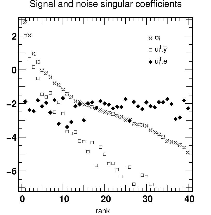
Figure 2: The decay of the singular values of the kernel (crosses) is the origin of the bad behaviour of the problem, through the amplification of the last singular vectors. In this example, the data $\mathbf{y}$ is perturbed by Gaussian noise of constant $\mathrm{SNR_{d}}=100$ per pixel. The unperturbed singular coefficients (white squares) decay, while the noise singular coefficients (black diamonds) remain spread around $1/\mathrm{SNR_{d}}$ for any $i$ (we chose $\langle\overline{\mathbf{y}}\rangle=1$ in this example). The perturbed singular coefficients $\mathbf{u}_{i}^{\top}\cdot\mathbf{y}$ are thus noise dominated as soon as $i\geq 7-9$, and so are the terms of the SVD solution (Eq. (22)). The increasing difference between the true and noise singular coefficients is worsened by the division by smaller $\sigma_{i}$. The solution $\mathbf{x}$ is dominated by the last few solution singular vectors, and its norm is purely noise dependent.

First, let us see how ill-conditioning arises, in the case of a noiseless kernel but with noisy data. We solve for $\mathbf{x}$ by maximizing the likelihood of the data $\mathbf{y}$ given the model; this is the same as minimizing:

$$\chi^{2}(\mathbf{y}|\mathbf{x})=\bigl{(}\mathbf{y}-\mathbf{B}\cdot\mathbf{x}\bigr{)}^{\top}\cdot\mathbf{W}\cdot\bigl{(}\mathbf{y}-\mathbf{B}\cdot\mathbf{x}\bigr{)}\,,$$ (17)

with respect to $\mathbf{x}$. The solution is the weighted least squares one:

$$\mathbf{x}_{\mathrm{ML}}=\bigl{(}\mathbf{B}^{\top}\cdot\mathbf{W}\cdot\mathbf{B}\bigr{)}^{-1}\cdot\mathbf{B}^{\top}\cdot\mathbf{W}\cdot\mathbf{y}\,.$$ (18)

For sake of simplicity, we will consider stationary noise in this section. The results of this section however apply for non-stationary noise by replacing the model matrix $\mathbf{B}$ by $\mathbf{K}{\cdot}\mathbf{B}$ and the data vector $\mathbf{y}$ by $\mathbf{K}{\cdot}\mathbf{y}$ where $\mathbf{K}$ is the Choleski decomposition of the weight matrix, i.e. $\mathbf{W}=\mathbf{K}^{\top}{\cdot}\mathbf{K}$. For stationary noise, the weight matrix factorizes out:

$$\chi^{2}(\mathbf{y}|\mathbf{x})\propto\bigl{(}\mathbf{y}-\mathbf{B}\cdot\mathbf{x}\bigr{)}^{\top}\bigl{(}\mathbf{y}-\mathbf{B}\cdot\mathbf{x}\bigr{)}\,,$$ (19)

and the maximum-likelihood solution becomes the ordinary least squares one:

$$\mathbf{x}_{\mathrm{ML}}=\bigl{(}\mathbf{B}^{\top}\cdot\mathbf{B}\bigr{)}^{-1}\cdot\mathbf{B}^{\top}\cdot\mathbf{y}\,.$$ (20)

In order to clarify the process of noise amplification, we introduce the singular value decomposition of $\mathbf{B}$ as:

$$\mathbf{B}=\mathbf{U}\cdot\mathbf{\Sigma}\cdot\mathbf{V}^{\top}\,,$$ (21)

where $\mathbf{\Sigma}=\operatorname{diag}(\sigma_{1},\sigma_{2},\dots,\sigma_{n})$ is a diagonal matrix carrying the singular values, sorted in decreasing order, of $\mathbf{B}$ on its diagonal. $\mathbf{U}$ contains the orthonormal data singular vectors $\mathbf{u}_{i}$ (data-size vectors), and $\mathbf{V}$ contains the orthonormal solution singular vectors $\mathbf{v}_{i}$ (solution-size vectors). Replacing $\mathbf{B}$ by its singular value decomposition in Eq. (20) yields:

$$\mathbf{x}_{\mathrm{ML}}=\mathbf{V}\cdot\mathbf{\Sigma}^{-1}\cdot\mathbf{U}^{\top}\cdot\mathbf{y}=\sum_{i=1}^{n}\frac{\mathbf{u}_{i}^{\top}\cdot\mathbf{y}}{\sigma_{i}}\,\mathbf{v}_{i}\,.$$ (22)

The solution is obtained as the sum of $n$ solution singular vectors $\mathbf{v}_{i}$ times the scalar $\mathbf{u}_{i}^{\top}\cdot\mathbf{y}/\sigma_{i}$. For real data, we have $\mathbf{y}=\overline{\mathbf{y}}+\mathbf{e}$, where the noiseless data $\mathbf{\overline{y}}$ is related to the true parameter vector $\overline{\mathbf{x}}$ via $\overline{\mathbf{y}}={\mathbf{B}}\cdot\overline{\mathbf{x}}$. Instead of $\overline{\mathbf{x}}$, the solution recovered from the noisy data reads:

$$\mathbf{x}_{\mathrm{ML}}=\sum_{i=1}^{n}\frac{\mathbf{u}_{i}^{\top}\cdot\mathbf{\overline{y}}}{\sigma_{i}}\,\mathbf{v}_{i}+\sum_{i=1}^{n}\frac{\mathbf{u}_{i}^{\top}\cdot\mathbf{e}}{\sigma_{i}}\,\mathbf{v}_{i}\equiv\mathbf{\overline{x}}+\mathbf{x}_{e}\,.$$ (23)

Thus, we recover the true unperturbed solution $\mathbf{\overline{x}}$ plus a perturbation, $\mathbf{x}_{e}$, related to the noise. Comparing $\mathbf{\overline{x}}$ and $\mathbf{x}_{e}$ is equivalent to comparing the unperturbed singular coefficients ${\mathbf{u}_{i}^{\top}\cdot\mathbf{\overline{y}}}$ and the noise singular coefficients ${\mathbf{u}_{i}^{\top}\cdot\mathbf{e}}$. Figure 2 shows an example with $40$ logarithmical age bins from $10$ Myr to $20$ Gyr, and where the data is perturbed by Gaussian noise and has constant $\mathrm{SNR_{d}}=100$ per pixel (the subscript d stands for data). The figure shows that the singular values decay very fast and span a large range, giving a conditioning number, defined by $\mathrm{CN}=\sigma_{1}/\sigma_{n}\approx 10^{8}$ characteristic of an ill-conditioned problem. Note that $\mathbf{B}$ is the flux-normalized SSP basis defined by Eq. (4), i.e. each spectrum of the basis has unitary flux, and the $x_{i}$ are thus flux fractions and not mass fractions (see Sect. 4.1.2 for more details). The noise singular coefficients remain rather constant for any rank $i$. Indeed, $\mathbf{u}_{i}^{\top}\cdot\mathbf{e}$ involves a normalized vector times noise, and has a constant statistical expected value of $\langle\overline{\mathbf{y}}\rangle/\mathrm{SNR_{d}}$. On the contrary, the unperturbed singular coefficients decay. In this example, the model $\overline{\mathbf{x}}$ is a Gaussian centered on $1$ Gyr, and we find that changing the mean age of the model does not significantly affect the decay of the ${\mathbf{u}_{i}^{\top}\cdot\mathbf{\overline{y}}}$ (see Appendix A). We can thus define two regimes, with a transition for $i_{0}\approx 7-9$ in this example:

• For $i\leq i_{0}$ we have ${\mathbf{u}_{i}^{\top}\cdot\mathbf{{y}}}\simeq{\mathbf{u}_{i}^{\top}\cdot\mathbf{\overline{y}}}$ and the singular coefficients and modes are set by the unperturbed signal $\overline{\mathbf{y}}$.

• For $i>i_{0}$ we have ${\mathbf{u}_{i}^{\top}\cdot\mathbf{{y}}}\simeq{\mathbf{u}_{i}^{\top}\cdot\mathbf{{e}}}\simeq\langle\overline{\mathbf{y}}\rangle/\mathrm{SNR_{d}}$. The singular coefficients are set by the noise in the data and saturate.

The division by decreasing $\sigma_{i}$ makes the high rank terms in $\mathbf{x}_{e}$ become very large. The solution $\mathbf{x}$ is thus dominated by the last few $\mathbf{v}_{i}$. Its norm is several orders of magnitude larger than the true solution. We see that, for such ill-conditioned problems, pure maximum-likelihood estimation results in huge noise amplification and useless solutions.

The origin of ill-conditioning is, in most part, physical: it lies in the evolution of the single stellar populations, which is dictated by stellar physics and the relevant stellar evolution models. One aspect of the situation is illustrated in Fig. 3. It shows a map of the $\chi^{2}$ distances between the spectra (i.e. columns) of the kernel $\mathbf{B}$, for different SNRs. In this figure, the time interval $[50$Myr$,15$Gyr$]$ was arbitrarily divided in $40$ logarithmic age bins, and the SSP basis is flux normalized as in Eq. (4). It shows that for low SNRs (of order 10), one element of the basis can not be quantitatively distinguished from its neighbours within a typical log age interval of $\sim$0.5 dex. It also makes it clear that the logarithmic age-resolution of any inversion method will not be constant all over the time range.

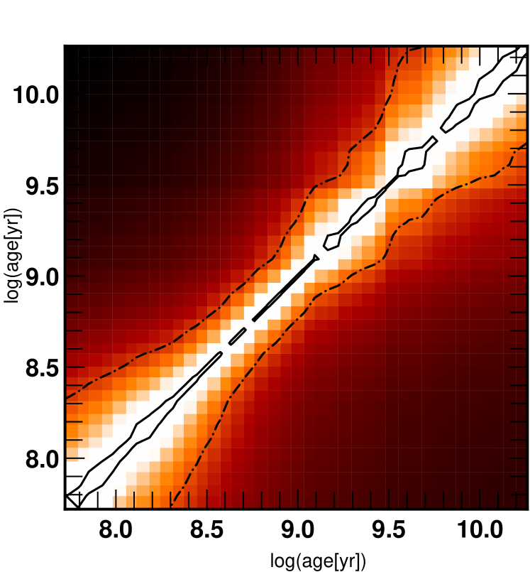
Figure 3: Distance map of the spectral energy distributions involved in the flux-normalized kernel $\mathbf{B}$. The contours enclose a domain where the $i$th spectrum can not be distinguised against the $j$th at a $90\%$ confidence level. The solid contour is for $\mathrm{SNR}=100$ per pixel and the dash-dotted one is for $\mathrm{SNR}=10$ per pixel. It is not possible to unambiguously disentangle two spectra in such regions, i.e. the resolution in age of any inversion method can not be finer than the width of these regions (which is read on the axis), and it is not constant all along the age range. This resolution in age in data space has a counter part in the resolution defined in Sect. 4.2

3.4.2 Noisy correlated kernel

Figure 4: Investigation of the noise signatures of the kernel. For comparison, the kernel was noised in several different ways: with white noise, oversampled noise and finally noise correlated in the age direction of the kernel, each type of noise producing characteristic features in the singular values. The expected spectral signature of the noise in the initial basis (saturation of the singular values) does not occur. This is likely to be caused by the interpolation between the stars of the stellar library: the noise patterns are carried along in the interpolation, giving rise to noise patterns correlated in the direction of ages.

As discussed in Sect. 2.3, the models which are constructed from observed spectra, are also contaminated by observational noise. Let us investigate the expected signature and basic properties of a noisy kernel.

PEGASE-HR single stellar populations have a noise component estimated to ${\mathrm{SNR_{b}}}\approx 200$ per $0.2$ Å pixel (the subscript b stands for basis). From theoretical studies of random matrices (Hansen, 1988), it is known that a hypothetical noiseless single stellar population basis perturbated by adding white noise of root mean square $\sigma_{0}$ should have its singular values settle around $\sqrt{m}\,\sigma_{0}$, where $m$ is the number of samples in the observed spectral energy distribution. If the spectra are normalized to unitary flux we have $\sigma_{0}\simeq 1/\mathrm{SNR_{b}}$. Figure 4 shows the singular values of the flux-normalized kernel $\mathbf{B}$ (thick line). The singular values clearly do not settle around the value expected for $m\simeq 10^{4}$, i.e. $\approx 1$ for $\mathrm{SNR_{b}}=100$ (dash-dotted line) and $\approx 0.1$ for $\mathrm{SNR_{b}}=1\,000$ (dash-double-dotted line). On the contrary, their decay is typical of an ill-conditioned noiseless kernel, as if the single stellar populations involved had infinite SNR. Let us investigate some details of the synthesis process, in an attempt to explain this unexpected property.

As every single stellar population is actually the weighted sum of $p$ single stars from the library, the noise level of the synthetic spectral energy distribution should be lower (typically divided by $\sqrt{p}$). However, the singular values of the kernel plus white noise at a level $\mathrm{SNR}=1\,000$ (corresponding to summing $p=100$ stars having $\mathrm{SNR}=100$) are still much larger than the initial kernel’s singular values. Having more stars available would lower the saturation level, but one would need $10^{10}$ stars with $\mathrm{SNR}=100$ to make the saturation vanish.

In order to test for the effect of wavelength resampling of the individual stellar spectra, we added $\mathrm{SNR}=100$ per pixel smoothed noise (i.e. noise with a correlation between neighboring wavelengths) to the kernel. The corresponding singular values are very similar to the former white noise case, except that they settle to a slightly smaller value. They still saturate high above the singular values of the initial kernel.

In contrast, when the added noise pattern is correlated in the direction of ages instead of wavelength, one obtains a non-saturated singular value spectrum very similar to the initial kernel, even with SNR as low as $100$ (a larger SNR would make it look even more similar).

Indeed, such correlated noise arises in part in the kernel because individual stellar spectra are interpolated in $(T,g,Z)$ space.

A single spectrum from the input stellar library can thus significantly contribute to several ages. For instance, the same limited number of red giants will be used (with slightly different weights) to represent the red giant branch stars over a range of ages and metallicities. Their noise patterns will show up in several consecutive synthetic single stellar populations, and can therefore not be properly discriminated against true physical signal. The expected saturation is washed out by the interpolation between spectra, resulting in a degraded signature. This correlation affects us in two ways: it prevents us from determining the precise SNR of the basis, and then from computing the conditioning number of the real problem (where $\mathrm{SNR_{b}}\rightarrow\infty$). Only a lower limit on the conditioning number is obtained, meaning the real problem could actually be worse.

Whatever process is responsible for degrading the noise signature, the properties of the problem in very high quality data regimes can not be inferred from the apparently noiseless initial kernel $\mathbf{B}$. Let’s return to the case of white noise, with a noisy kernel $\mathbf{B+E}$. Its singular values saturate at some rank $i_{B}$. The singular vectors of lower rank are identical to those of $\mathbf{B}$ but for higher rank, they differ strongly. Thus, the number of free parameters we can recover can not be larger than $i_{B}$. For Pégase-HR we estimate $i_{B}=6$ for $\mathrm{SNR_{b}}\approx 200$. This means that high frequency variations of the stellar age distribution are unreachable, no matter what is the SNR of the data. This is a fundamental limitation of the problem, related specifically to the SNR of the single stellar population models. When $\mathrm{SNR_{d}}\geq\mathrm{SNR_{b}}$, a pure maximum likelihood estimation actually uses noise patterns inside the kernel as if it was true physical signal, and simulations will give results with an illusory accuracy. A useful technique, which explicitly accounts for modeling errors, is then total least squares (hereafter TLS). The total least squares solution to our linear problem (for simplicity we set $\mathbf{W}$ to Identity here) is defined by:

$$\mathbf{x}_{\mathrm{TLS}}=\arg\min_{\mathbf{x},\,\bar{\mathbf{B}}}\,\left(\|\mathbf{y}-\bar{\mathbf{B}}\cdot\mathbf{x}\|^{2}+\|\bar{\mathbf{B}}-\mathbf{B}\|^{2}\right)\,,$$ (24)

where $\|\mathbf{x}\|=\sqrt{\mathbf{x}^{\top}\cdot\mathbf{x}}$ denotes the Euclidian (or $\ell_{2}$) norm. More can be found in Hansen & O’Leary (1996) and Golub et al. (2000).

However, in the rest of the paper, we will most frequently explore regimes where the dominant error source is the data, so that the number of degrees of freedom of the problem is dictated by $\mathrm{SNR_{d}}$ rather than $\mathrm{SNR_{b}}$. It will also allow us to estimate what could be the best performance of the method, if the single stellar population models were taken as perfect. Thus, in the following sections, we will focus exclusively on the treatment of noisy data, and will often drop the subscript “d”.

3.5 Regularization and MAP

This section explains how adequate regularization allows us to improve the behaviour of the problem with respect to noise in the data. Perturbation of the solution arises from the noise-dominated higher rank terms of Eq. (22). In order to ensure that $\mathbf{x}_{e}$ remains small, one could reduce the effective number of age bins. Several criteria are applicable.

• The singular coefficients should always be dominated by the true signal. With plots such as Fig. 2, we find that $i_{0}$ is between $7$ and $9$ for $\mathrm{SNR_{d}}=100$ per pixel with Pégase-HR single stellar populations. Nevertheless, in a real situation only $\mathbf{u}_{i}^{\top}{\cdot}\mathbf{y}$ is generally available, and $i_{0}$ is guessed from the rank for which the singular coefficients begin to saturate.

• In the true signal dominated region, the singular coefficients decrease faster than the singular values. Inversely, singular coefficients decreasing faster than the singular values for any rank $i$ guarantee the smallness of $\mathbf{x}_{e}$. This requirement is known as the discrete Picard condition. See Hansen (1994) for further details.

• A useful criterion that does not require any plot involves choosing the number of age bins $n$ so that the conditioning number of the resulting kernel satisfies

  $$\mathrm{CN}=\sigma_{1}/\sigma_{n}\lesssim\sqrt{m}\,\mathrm{SNR_{d}}\,,$$ (25)

  where ${m}$ is the number of pixels.

Note that this statement is SNR dependent.

Another way to prevent the noise component from being amplified into the solution is to truncate the SVD expansion at some rank $i_{\mathrm{trunc}}$:

$$\mathbf{x}_{\mathrm{TSVD}}=\sum_{i=1}^{i_{\mathrm{trunc}}}\frac{\mathbf{u}_{i}^{\top}\cdot\mathbf{y}}{\sigma_{i}}\,\mathbf{v}_{i}\,.$$ (26)

This technique is known as truncated SVD (hereafter TSVD). The use of this method dates back to Hanson (1971) and Varah (1973). The truncation rank $i_{\mathrm{trunc}}$ can be chosen with the help of plots such as Fig. 2

However, if the truncation is brutal, it will produce strong artifacts, known as aliasing, which reflects the fact that higher frequencies are projected onto a low frequency basis; the best fit leads to a non local alternated expansion which rings. Moreover, TSVD is best suited for problems where a clear gap in the singular values is seen because in this instance, the lower modes are well represented by the truncated basis. Unfortunately, our kernel displays a smooth, continuously decreasing spectrum of singular values. This is very similar to the situation in image reconstruction. When deconvolution problems are addressed, the brutal truncation of the transfer function (which corresponds to the singular coefficients of the point spread function, hereafter PSF) results in the formation of strong artifacts known as Gibbs rings.

Moreover, we here have an other degree of complexity arising from the property that our problem is not shift-invariant. As a consequence, the solution singular vectors are fairly unsmooth and even more artifacts are expected as discussed in Sect. 4.1.2. In image deblurring, artifacts are reduced and reconstructions improved by apodizing the Fourier transformed PSF (i.e. making it smoothly decrease to $0$), for example by Wiener filtering. In a similar manner, we wish to apodize the singular value spectrum of the kernel $\mathbf{B}$.

We chose to regularize the problem by imposing the smoothness of the solution through a penalizing function. We define the objective function as

$$Q_{\mu}(\mathbf{x})\equiv-\frac{1}{2}\log(f_{\mathrm{post}})={\chi^{2}}({\mathbf{s}}(\mathbf{x}))+\mu\,P(\mathbf{x})\,,$$ (27)

which is a penalized $\chi^{2}$, where $P$ is the penalizing function: it has large (small) values for unsmooth (smooth) $\mathbf{x}$. Adding the penalization $P$ to the objective function is exactly equivalent to injecting a priori information in the problem. We effectively proceed as if we assumed a priori that a smooth solution was more likely than a rough one. This is in part justified by the fact that any unregularized inversion tends to produce rough solutions. If we identify $Q_{\mu}$ with the expression of the logarithm of the maximum a posteriori likelihood (16) we see that by building a penalization $P$ we have built a prior distribution $f_{\mathrm{prior}}$

$$f_{\mathrm{prior}}({\mathbf{x}})=\exp\left(-\mu P({\mathbf{x}})\right)\,,$$ (28)

omitting the normalization constant. If $\mu=0$, the prior distribution is uniform and contains no information. It is a pure maximum likelihood estimation. If $\mu>0$ the prior probability density is larger for smooth solutions, and we are performing a maximum a posteriori likelihood estimation (MAP).

The smoothing parameter $\mu$ sets the smoothness requirement on the solution. There are several examples of such regularizations in the litterature (Tikhonov, least squares with quadratic constraint, maximum entropy regularization …see Pichon et al. (2002) for a discussion). Here, we define $P$ as a quadratic function of $\mathbf{x}$, involving a kernel $\mathbf{L}$.

$$P(\mathbf{x})=\mathbf{x}^{\top}\cdot\mathbf{L}^{\top}\cdot\mathbf{L}\cdot\mathbf{x}\,,$$ (29)

If $\mathbf{L}$ is the identity matrix $\mathbf{I}_{n}$, then $P(\mathbf{x})$ is just the square of the Euclidian norm of $\mathbf{x}$. To explicitly enforce a smoothness constraint, we can use a finite difference operator $\mathbf{D}_{2}\equiv{\operatorname{diag}}_{2}[-1,2,-1]$ that computes the Laplacian of $\mathbf{x}$, defined in Pichon et al. (2002) by

$$\mathbf{D}_{2}\equiv\left[\begin{array}[]{rrrrrrrr}-1&2&-1&0&0&0&0&\cdots\cr 0&-1&2&-1&0&0&0&\cdots\\ 0&0&-1&2&-1&0&0&\cdots\\ 0&0&0&-1&2&-1&0&\cdots\\ \cdots&\cdots&\cdots&\cdots&\cdots&\cdots&\cdots&\cdots\end{array}\right]\,\,\,\,,$$ (30)

The objective function $Q_{\mu}$ is then quadratic and has an explicit minimum:

$$\mathbf{x}_{\mu}\triangleq\widetilde{\mathbf{B}}\cdot\mathbf{y}=\Bigl{(}\mathbf{B}^{\top}\cdot\mathbf{W}\cdot\mathbf{B}+\mu\,\mathbf{L}^{\top}\cdot\mathbf{L}\Bigr{)}^{-1}\cdot\mathbf{B}^{\top}\cdot\mathbf{W}\cdot\mathbf{y}\,,$$ (31)

where $\widetilde{\mathbf{B}}$ is defined here to be the regularized inverse model matrix, whose properties we will investigate below.

We may now derive a more insightful expression for $\mathbf{x}_{\mu}$ while relying on the generalized singular value decomposition(hereafter GSVD) of $(\mathbf{B},\mathbf{L})$ (assuming $\mathbf{W}=\mathbf{I}_{m}$ or using the Choleski square root of $\mathbf{W}$). According to Appendix C, the regularized solution now writes:

$$\mathbf{x}_{\mu} = \arg\min_{\mathbf{x}}\left(\|\mathbf{B}\cdot\mathbf{x}-\mathbf{y}\|^{2}+\mu\,\|\mathbf{L}\cdot\mathbf{x}\|^{2}\right)\,,$$ (32)

$$= \bigl{[}\mathbf{B}^{\top}\cdot\mathbf{B}+\mu\,\mathbf{L}^{\top}\cdot\mathbf{L}\bigr{]}^{-1}\cdot\mathbf{B}^{\top}\cdot\mathbf{y}\,,$$

$$= \mathbf{V}\cdot\bigl{[}\mathbf{\Sigma}^{2}+\mu\,\mathbf{\Theta}^{2}\bigr{]}^{-1}\cdot\mathbf{\Sigma}\cdot\mathbf{U}^{\top}\cdot\mathbf{y}\,,$$

$$= \sum_{i=1}^{n}\eta_{i}\,\bigl{(}\mathbf{u}^{\top}_{i}\cdot\mathbf{y}\bigr{)}\,\mathbf{v}_{i}\,,$$

where the filter factors $\eta_{i}$:

$$\eta_{i}=\frac{\sigma_{i}}{\sigma_{i}^{2}+\mu\,\theta_{i}^{2}}\,,$$ (33)

depend on the type of penalization and the smoothness parameter $\mu$. For any quadratic penalization as in Eq. (29), the matrices $\mathbf{U}$, $\mathbf{V}$, $\mathbf{\Sigma}=\operatorname{diag}(\sigma_{1},\sigma_{2},\dots,\sigma_{n})$ and $\mathbf{\Theta}=\operatorname{diag}(\theta_{1},\theta_{2},\dots,\theta_{n})$ are given by the generalized singular value decomposition of the matrix pair $(\mathbf{B},\mathbf{L})$ (see Appendix C for details). For the simple case of square Euclidian norm penalization, $\mathbf{L}=\mathbf{I}_{n}$, the filter factors becomes:

$$\eta_{i}=\frac{\sigma_{i}}{\sigma_{i}^{2}+\mu}\,.$$ (34)

We then have $\eta_{i}\approx 1/\sigma_{i}$ when $\sigma_{i}^{2}\gg\mu$, and $\eta_{i}\rightarrow 0$ for higher ranks (i.e. smaller singular values), so that division by almost $0$ is avoided in high rank terms. Thus, setting $\mu$ actually sets the rank where the weights of the SVD solution components begin to decrease. Note that the smooth cutoff (apodization) of the singular values should allow us to recover models similar to relatively high rank singular vectors provided that the weights associated to lower rank vectors are small enough. Small $\mu$ yield noise sensitive, possibly unphysical solutions, whereas very large $\mu$ lead to flat solutions whatever the data. The choice of $\mu$ thus appears as a critical step, and should give a fair balance between smoothness of the solution and sensitivity to the data.

3.6 Setting the weight for the penalty: $\mu$

The optimal weighing between prior and likelihood is a central issue in MAP since it allows us to taylor the effective degree of freedom of each inversion to the SNR of the data. See, e.g., Titterington (1985) for an extensive comparison between various methods for choosing the value of the hyper-parameter $\mu$.

3.6.1 The automatic way: generalized cross validation

Figure 5: Histograms of the distribution of $\mu_{\mathrm{GCV}}$ for a linear stellar age distribution inversion with 60 age bins, and several SNR per pixel and penalizations. From left to right: Euclidian norm, Laplacian and $\mathbf{D}_{3}$ penalizations. The distributions are vertically offset for readility, and the SNR is given for each of them. The median of these distributions give the GCV-optimal smoothing parameter for each SNR and penalization. It is well defined in all cases except for very low $\mathrm{SNR}=5$ per pixel. The median parameter increases with the order of the penalization and decreasing SNR. Note the skewed distributions (this is quite generic in GCV).

Generalized cross validation (GCV) is a function of the parameter $\mu$, the data and the kernel $\mathbf{B}$, defined as

$${\mathrm{GCV}}(\mu)=\frac{\bigl{\|}\bigl{(}\mathbf{I}-\mathbf{B}\cdot\tilde{\mathbf{B}}\bigr{)}\cdot\mathbf{y}\bigr{\|}^{2}}{\operatorname{tr}^{2}\bigl{(}\mathbf{I}-\mathbf{B}\cdot\tilde{\mathbf{B}}\bigr{)}}\,,$$ (35)

where $\tilde{\mathbf{B}}$ is the regularized inverse model, defined by Eq. (31) and $\operatorname{tr}(\cdot)$ is the trace of its argument. The minimum of GCV optimizes the predictive power of the solution (Wahba, 1990), in the sense that if any pixel is left out of the data, this pixel’s value should still be well predicted by the corresponding regularized solution. For quadratic penalizations, one may obtain very simple expressions for the GCV function, speeding up its computation, and therefore the determination of $\mu$ by several orders of magnitude. Using the GSVD of $(\mathbf{B},\mathbf{L})$, we can derive:

$$\mathrm{GCV}(\mu)=\frac{\sum_{i=1}^{n}\left(\rho_{i}\,\mathbf{u_{i}}^{\top}\cdot\mathbf{y}\right)^{2}}{\left(\sum_{i=1}^{n}\rho_{i}\right)^{2}}\,,$$ (36)

where

$$\rho_{i}=1-\frac{\sigma_{i}^{2}}{\sigma_{i}^{2}+\mu\,\theta_{i}^{2}}=\frac{\mu\,\theta_{i}^{2}}{\sigma_{i}^{2}+\mu\,\theta_{i}^{2}}\,.$$ (37)

where $\sigma_{i}$ and $\theta_{i}$ are the singular values obtained from the generalized singular value decomposition of the matrix pair $(\mathbf{B},\mathbf{L})$ (see Appendix C). Note that the $\mu$ in the denominator of $\rho_{i}$ factorizes out in the expression of $\mathrm{GCV}(\mu)$.

When available, the minimum of GCV provides a good, data quality-motivated value for $\mu$. Moreover, GCV has been extendedly tested and applied by a number of authors, in several fields of physics. Figure 5 shows distributions of $\mu_{\mathrm{GCV}}$ for a mono-metallic inversion for several SNR and penalizations. Each histogram results from $150$ experiments. The GCV determination of the smoothing parameter is successful over a wide range of SNR, in the sense that the histogram shows a clear maximum. This maximum is best defined for the Tikhonov penalization (square of the Euclidian norm). With laplacian and higher order penalizations, especially for low SNR, the GCV values are more widely spread. Nevertheless, we can still obtain a useful value by extrapolating the higher SNR $\mu$ down to the desired SNR.

3.6.2 Empirical approach: trial and error

GCV and most of the automated smoothing parameter choice methods were designed for linear problems. In the case of non-linear problems, it can provide a useful value for $\mu$ to start with, but fine empirical tuning is also required (Craig & Brown, 1986). For instance, when positivity is imposed through reparameterization or gradient clipping, $\mu$ should be smaller than $\mu_{\mathrm{GCV}}$. Indeed, since the positive problem has a better behaviour than the full linear one, it is expected that GCV overestimates $\mu$. One can thus afford to lower it to some extent without threatening the relevance of the solution. As a consequence, finer structures can be recovered. To set $\mu$ for the positive problem, we used the simple following procedure. First, we set $\mu=\mu_{\mathrm{GCV}}$. We produce mock data, and perform successive inversions, while decreasing $\mu$. As a consequence, finer structures are recovered. At some point, we will enter a regime where the structures of the solution can be identified as artifacts. This transition defines a lower limit above which $\mu$ should remain.

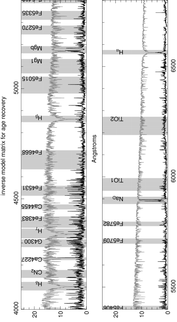
Figure 6: Black solid line: peak to peak variations of the inverse model matrix discussed in Sect. 3.7. In this example, we took $60$ age bins and $\mu=10^{2}$ corresponding to $\mathrm{SNR}=100$ per pixel with Laplacian penalization. Large values point at age-sensitive parts of the spectrum. A $500$ Myr single stellar population with half-solar metallicity is shown as reference (grey solid line). The spectral domains corresponding to the Lick indices appear as grey-shaded areas. Many of the spectral domains involved in the Lick system seem to effectively carry more information than the rest of the spectrum. However, the information is still widely distributed along the whole optical range.

3.7 Where is the age information?

Which spectral domains or lines are most discriminative in terms of population age-dating? An answer to this can be given by inspecting the properties of the regularized inverse model matrix $\tilde{\mathbf{B}}(\mu)$ defined by Eq. (31). In effect, we expect the peak to peak amplitude of a column of $\tilde{\mathbf{B}}(\mu)$ to be largest for the most discriminatory wavelengths for age-dating. In Fig. 6, the inverse model matrix was computed for a Laplacian penalization with $\mu_{\mathrm{GCV}}=10^{2}$ corresponding to $\mathrm{SNR}=100$ per pixel with $60$ age bins from $10$ Myr to $20$ Gyr and half-solar metallicity. It shows that the Balmer lines ${\mathrm{H}}_{\alpha,\beta,\gamma,\delta}$, along with the spectral regions of the Lick index NaD, the magnesium indices ${\mathrm{Mg}}_{1},{\mathrm{Mg}}_{2},{\mathrm{Mg}}_{b}$ and the calcium ${\mathrm{Ca}}_{4227}$ have strong weight in the age-dating process. Note that the above analysis is clearly noise dependent via $\tilde{\mathbf{B}}(\mu_{\mathrm{GCV}})$. The list of relevant lines will change with the SNR. Many of the wiggles and peaks of the inverse model remain so far uninterpreted, and many peaks hit spectral domains where no referenced index is known, but still contribute strongly to age separation. Another important feature of the inverse model is that most of its norm is in the form of low value pixels. If some of the peaks were $2$ or $3$ orders of magnitude larger than the average value, we could conclude that most of the information is contained exclusively in the corresponding lines. Yet, the Fig. 6 does not allow us to reach this conclusion. Even though the information seems denser in the strongest, well known lines, most of it remains in the form of a large number of weaker lines, more concentrated in the blue part of our spectra. This supports the intuition that a lot of information is left aside by looking exclusively at spectral indices, and that the constraints obtained therefrom are not optimal. Hence our effort to build a global spectrum fitting tool.

4 Validation: Behaviour of the linear inversion

Let us now apply STECMAP to mock data, to study the biases and the dispersion of the solutions, and to test for different penalizations. Producing mock data involves choosing a model age distribution, $\mathbf{x}_{M}$, and a noise model, $\mathbf{e}$. A mock spectrum is then obtained as $\mathbf{y}=\mathbf{B}\cdot\mathbf{x}_{M}+\mathbf{e}$. The corresponding astrophysical goal is the recovery of the star formation history of mono-metallic stellar populations (for example superimposed clusters) seen without extinction. The stellar age distribution models for these objects are single (Sect. 4.1) or multiple (Sect. 4.2) star formation episodes of approximately Gaussian shape. Recall that no assumption on the shape of the distribution is included in the inversion process. The only a priori is the smoothness of the solution, while the smoothing parameter is set by GCV. Here we relate the results of our simulation to the properties of the solution singular vectors, thereby explaining the generation of artifacts.

4.1 Single bump stellar age distribution

Let us discuss in turn the relationship between the artifacts of the reconstructions and the shape of the solution vectors (Sect. 4.1.1), the flux-averaging of the basis and the behaviour of the problem regarding the fiducial model (Sect. 4.1.2), the choice of penalization (Sect. 4.1.3), the requirement to impose positivity (Sect. 4.1.4), and the need for an extensive simulation campaign (Sect. 4.1.5)

4.1.1 Artifacts and the shape of the solution vectors

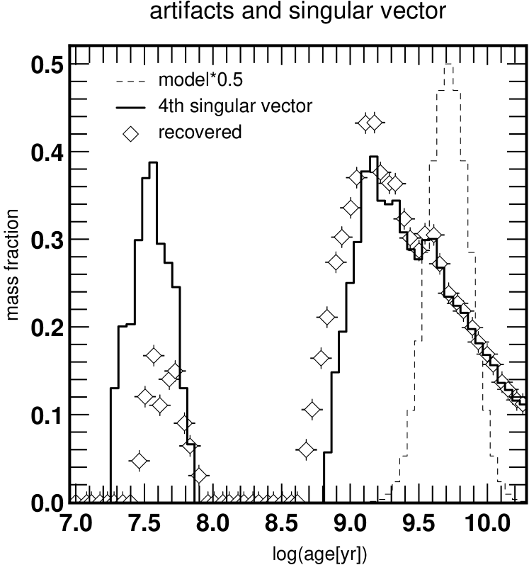
Figure 7: Blow-up of the bottom right panel of Fig. 8 showing only the mass reconstruction of the oldest bump. The dashed line is the model distribution, and the diamonds show the median of the recovered age distributions for $10$ realizations. The error bars showing the dispersion are smaller than the symbol itself. The details of the shape of the mass distribution reconstruction trace closely the $4$th singular vector of the kernel $\mathbf{B}$, with very little dispersion, showing that the artifacts and the fine structures of the reconstructions are closely related to the properties of the single stellar population models.

Since any solution is a linear combination of the solution vectors $\mathbf{v}_{i}$ (see Eq. (32)), their shapes impose what kind of shape for $\mathbf{x}$ can or can not be reconstructed, depending on what feature in the observed spectra is best matched by the corresponding data singular vectors.

Moreover, as regularizing the problem involves attenuating the high rank terms of Eq. (32), the detailed shape of the solution is in general given by the first few $\mathbf{v}_{i}$. Figure 7 shows the stellar mass distribution reconstruction of an old population. It is actually a blow-up of the recovery of the oldest burst in the bottom right panel of Fig. 8. The penalization is square Euclidian norm, so that the relevant singular vectors are given by the SVD of $\mathbf{B}$. The details of the solution are mostly those of the $4$th solution singular vector, and appear as a systematic artifact (the diamonds are the median of $10$ realizations, and the dispersion of the solutions is smaller than the symbol itself). The spurious young component between $10^{7.5}$ and $10^{8}$yr seems to be related to the 4th singular vector as well, and also appears systematically even though it has no physical reality. The fine structure and the artifacts of any solution thus rely most on the properties of the single stellar population basis rather than on the data or even the realization of the noise.

It is generally impossible to reconstruct accurately the shape of the distribution for ages where the singular vectors display no structure. The right panel of Fig. 9, shows that the $10$ first singular vectors of the absolute flux kernel have very little structure for ages larger than $\simeq 3$ Gyr. Correspondingly, the right panels of Fig. 8 show that indeed, in this range of ages, the shape of the distribution is very poorly constrained.

For an inversion problem to be well behaved, the first solution singular vectors, the $\mathbf{v}_{k}$, should be rather smooth. They should display more and more oscillations as the rank $k$ increases (typically $k-1$ oscillations), but remain smooth and regular. The unsmooth aspect of our singular vectors arises from the temporal roughness in the spectral basis. This could also be related to physical fast evolution of the single stellar populations in some specific stages of stellar evolution, producing variable distance between the elements of the basis. It also reflects the non shift-invariance of the problem, as is also illustrated by Fig. 3.

Some further artifacts can however not be trivially explained by the solution singular vectors alone. For example many of the displayed solutions, even with high SNR, show variations far away from the bulk of the signal, seen as misleading spurious secondary bumps. This artifact is the analog of Gibbs rings in imaging. It arises because the higher frequency modes needed to suppress these secondary oscillations are attenuated by regularization, and would be best identified by examining the GSVD of $(\mathbf{B},\mathbf{L})$. It is the old age extension of the low frequency mode involved in building the main bump. We will deal with this by introducing positivity in Sect. 4.1.4.

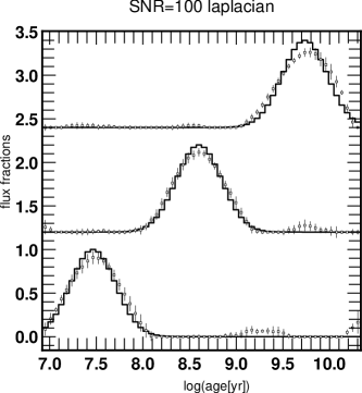
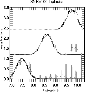
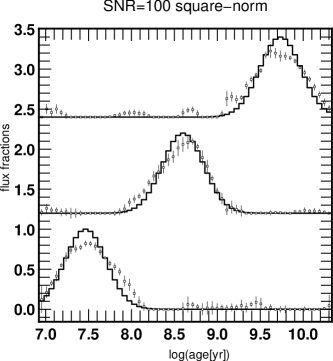
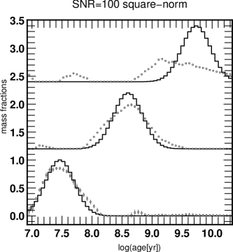
Figure 8: Simulations of the reconstruction of a young, intermediate and old single burst populations. The thick histograms represent the models, while the symbols and vertical bars show the median and interquartiles of 10 inversions. Negative values in these reconstructions have been set to zero for clarity. Right: Case of an absolute flux basis. The plots thus represent mass fractions. Left: Case of a flux normalized basis. Thus are represented flux contributions. The SNR is fixed to $100$ per pixel with $R=10\,000$. The penalizations are square Euclidian norm (bottom) and Laplacian (top). In terms of distance to the model, the bumps are best reconstructed in flux fractions, and the best penalization is Laplacian. We checked that Laplacian penalization gave flux fraction reconstructions similar to the third order penalization, showing that these do not strongly rely on the details of the smoothness a priori.

4.1.2 Flux-normalized basis and independence from the fiducial model

Figure 9: Solution singular vectors of the flux-normalized kernel (left) and the absolute flux basis (right). The vectors are vertically offset for lisibility, and the associated singular values are given on the right. The low rank singular vectors of the absolute flux basis are very flat in the large ages, indicating that no information about these populations can be obtained unless we have very high SNR. On the contrary, fluctuations in large ages are already present in the low rank singular vectors of the flux-normalized basis, which indicates the better feasibility of reconstructing the age distribution in the older part.

In practice, one can choose between a basis where the flux of each single stellar population is given for $1M_{\sun}$ (absolute flux basis or mass-normalized basis), and a basis where the flux of each single stellar population has been normalized to the same value (or flux-normalized basis, cf. Sect. 2.1). This choice has a physical meaning: in the first case, the unknown $\mathbf{x}$ will contain mass fractions, whereas in the latter case, it will contain flux fractions.

There are several reasons why we prefer to work with the flux-normalized basis.

It is more directly linked to the luminous properties of the observed population (and thus less directly linked to the mass): a component of a given flux can not “hide” behind another component of similar flux. This is not true for components of similar masses, due to the evolution of $M/L(t)$. For instance, in the upper right plot of Fig. 8, the mass of the older components is poorly constrained when the model is a young burst. This is expected, because when a young component is present, adding the same mass of old stars will have very little effect on the integrated optical light. This is predictable from the lack of structure beyond $3$ Gyr in the singular vectors of the right panel of Fig. 9 (see also the discussion in Sect. 4.1.1). Modulations in this range of ages are seen in the vectors of the right panel for the higher rank vectors only. On the other hand, the singular vectors of the flux-normalized basis (left panel of Fig. 9) display structure in the large ages even for low ranks, indicating a better behaviour. And indeed, the upper left plot of Fig. 8 shows that all the flux fractions are satisfactorily constrained no matter if the model population is young or old. In this respect, the “separability” issues tackled later in the article for superimposed populations (Sect. 4.2) are more easily discussed in terms of flux fractions. Note that it is however not expected that the mass fractions obtained by multiplying the flux fractions by $M/L(t)$ be accurate over the whole age range (positivity will improve this particular aspect significantly; see Sect. 4.1.4).

The difference of behaviour between the mass and flux fractions reconstructions is also reflected in the variation of the transition rank $i_{0}$ (see Sect. 3.4) between the noise and signal dominated regimes, as shows Fig. 21. For a mass-normalized basis, the transition rank $i_{0}$ increases with the age of the fiducial model $\overline{\mathbf{x}}$ (as defined in Panter et al. (2003)), from 5 to 20. On the other hand, for a flux-normalized basis, the transition rank remains around 7-9 in this pseudo-observational setup, no matter the age of the fiducial model. Ideally, we would like to come up with a problem whose behaviour is fixed only by the SNR. In this respect, independence of the transition rank $i_{0}$ from the fiducial model is a welcome property. We thus chose to carry on with the flux-normalized basis for the rest of the paper.

4.1.3 Laplacian or square Euclidian norm penalty

Figure 8 allows us to check which penalization gives the solutions with smallest distance to the model. First of all, it is quite clear that the square Euclidian norm penalization is worst, because it produces both flattened solutions and strong artifacts. Indeed, requiring the norm of the solution to be small does not explicitly have an effect on the smoothness of the solutions.

Laplacian penalizations give results very similar to the third order penalization $\mathbf{D}_{3}\equiv{\mathrm{Diag}}_{3}[-1,3,-3,1]$ defined as in Eq. (30) . The latter are therefore not plotted, and perform equally well at any SNR. Both produce moderately flattened solutions showing increasing dispersion with decreasing SNR, without systematic bias in age. The width of these bumps is a simple (but crude) measure of the time resolution of the reconstructions, because any bump narrower than the models displayed would be broadened by the inversion. The absence of significant difference between the results of the Laplacian and third order penalizations shows that the inversion does not rely strongly on the details of regularization, as long as it involves a differential operator. We chose to carry on with the Laplacian penalization for the rest of the paper.

4.1.4 Positivity and Gibbs apodization

Positivity of the solution is a physically motivated requirement, but it also stabilizes the inversion by strongly reducing the explored parameter space. The maximum frequency (or best resolution in age) that would be obtained for infinite SNR is thus not only a matter of basis ill-conditioning but also has a methodological component. This is illustrated by the slightly better age-resolution (and thus higher frequency) obtained while relying on positivity as shown in Fig. 10. Unfortunately there isn’t any simple extension of the analytical ill-conditioned problem diagnosis to the non linear problem. Also the minimization of $Q_{\mu}$ defined in Eq. (27) requires efficient algorithms as described in Appendix B. As any regularization method, positivity will also introduce some bias. Indeed, the solutions in Fig. 10 seem to be slighlty asymmetrical compared to the linear solutions. However, one strong advantage of positivity is its ability to reduce Gibbs ringing. Linear solutions with any penalization exhibit spurious oscillations even far from the main bump, which can be interpreted as a superimposed component. These annoying artifacts do not appear in the positive solutions as shows Fig. 10. In many applications, this property turns out to be more important than the possible bias it might introduce in age estimation.

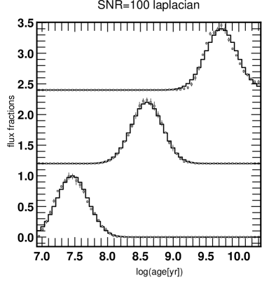
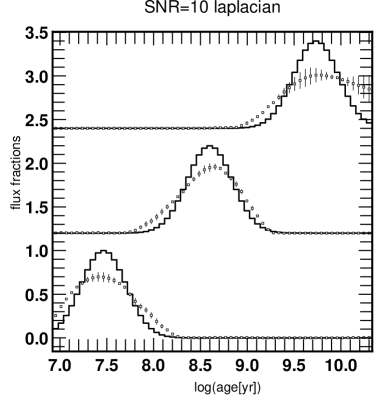
Figure 10: Same as Fig. 8 with a flux-normalized basis, positivity enforced by quadratic reparameterization and Laplacian penalization. Results of simulations for $\mathrm{SNR}=100$ and $\mathrm{SNR}=10$ per pixel at $R=10\,000$ are shown. Even though some residual remains, the solution sticks to zero where it should, instead of displaying Gibbs rings.

4.1.5 Why carry out an extensive simulation campaign?

An inversion method can perform very well for some specially chosen cases while performing poorly generally. As an example we discuss the recovery of the age distribution of a complex population consisting in a superposition of young, intermediate, and old sub-populations. Each of these 3 components contributes equally to the total observed spectrum $\mathbf{y}$. The noise is Gaussian. Figure 11 shows reconstructions of the age distribution by the Eq. (31), for 150 realizations, with a Laplacian penalization. The reconstruction seems to be satisfactory: it is unbiased and the interquartile intervals of the solutions shrink with increasing SNR. A naive reading of Fig. 11 would suggest that we are able to recover nearly any age distribution, without bias and with very small error for all the time bins, even with quite low SNR, but there is a trick. Why do the simulations in Fig. 11 look so good? First, the temporal frequency of the solution is lower than in the single bump simulations. Second, higher frequency sine fuctions are needed to represent a single bump than to represent a sinusal curve (one is enough). Thus, as the first singular vectors roughly form a basis of sine functions, one needs fewer and lower order solution singular vectors to represent a sine function than a bump, and lower SNR.

One simple (yet unadvisable!) recipe to make good looking simulations even without regularization could involve the following steps:

1. choose as model $\mathbf{x}$ one of the last few solution singular vectors $\mathbf{v}_{k}$ (or one of the first few if some penalization is implemented)

2. compute the corresponding pseudo-data $\mathbf{y}=\mathbf{B}\cdot\mathbf{x}$

3. noise the data at chosen SNR

4. invert and show how close the recovered solution lies to the initial model

By doing so, we managed to produce apparently good looking simulations down to $\mathrm{SNR}=0.1$ per pixel. Thus the requirement to assess and demonstrate the validity and efficiency of the MAP method carried out in this section.

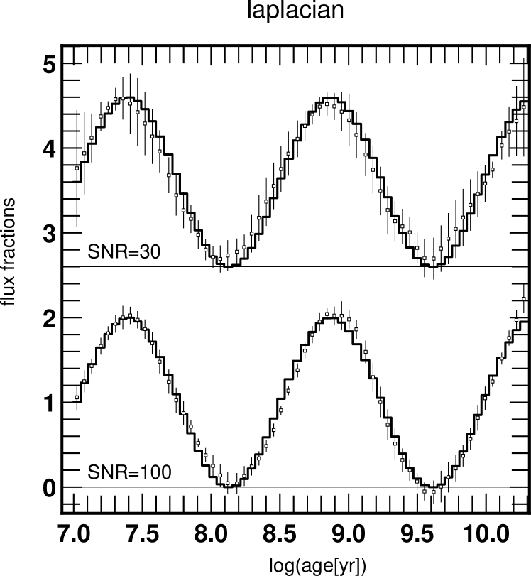
Figure 11: Same as Fig. 10, with a $1+\sin$ model for the stellar age distribution. The SNR per pixel is given for each experiment ($10$ realizations), and the resolution is $R=10\,000$. The smoothing parameter $\mu$ was adjusted by running several simulations and choosing the one providing the smallest distance to the model. The reconstruction is excellent, but there is a catch: it turns out that sine functions are intrinsically easier to recover than single bumps, given the shape of the solution vectors of the kernel. Hence, such reconstructions are very misguiding. More systematic simulations are required.

4.2 Age separation versus $R$ and SNR

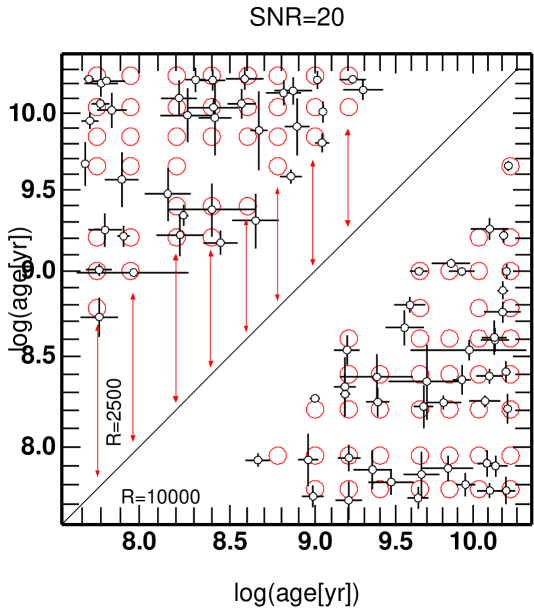
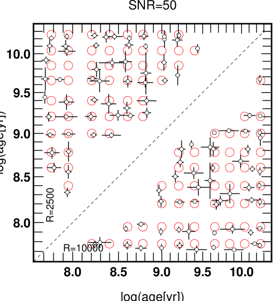
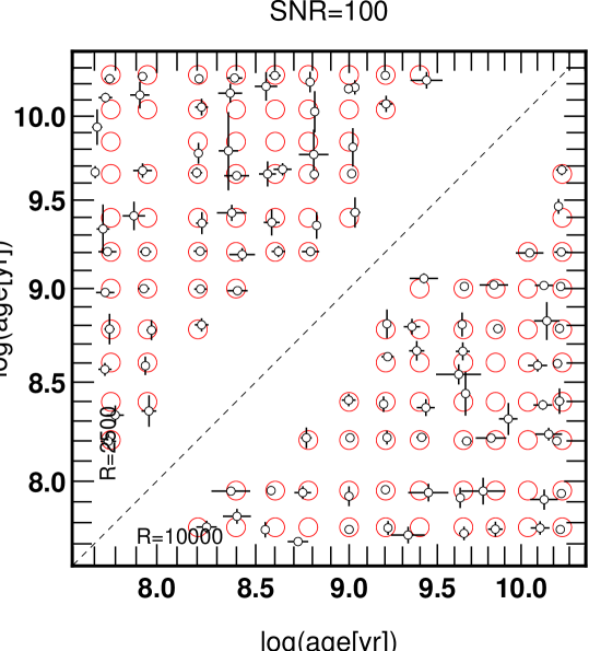
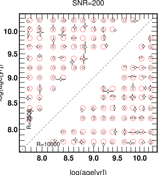
Figure 12: Recovery of double bursts for several SNR per Å. The large circles are the models. Their coordinates $(a_{1},a_{2})$ are the ages of the two bursts. The smaller circles with error bars show the median and the interquartiles of the recovered ages in $10$ reconstructions each. The dotted line represents the $a_{1}=a_{2}$ limit. Solutions that do not satisfy the quality criteria illustrated in Fig. 14 are rejected and not plotted. The upper diagonal part of each panel shows $R=2\,500$ results while the lower diagonal part shows $R=10\,000$ results. Results for the other spectral resolutions down to $R\approx 1\,000$ are very similar and therefore not shown. Our ability to separate close double bursts improves with increasing SNR, but does not significantly change with spectral resolution. The top left panel illustrates the definition of the resolution in age as the median length of the segments. Note that the shape of the “unseparable” zone and its evolution with SNR are similar to that shown in Fig. 3.

We have already made clear that we can not recover all the high frequency oscillations of a given stellar age distribution even with very high SNR, but rather moderately slow variations, corresponding to smooth solutions. Let us nonetheless consider the special case where a composite population consists of two successive bursts, i.e. stellar age distributions with two bumps of same luminosity. This is one order of complexity above the classical characterization of a population through one unique age using Lick indices. And indeed, it applies to many astrophysically interesting cases. The ability to separate the two main populations would allow for example to age-date respectively the disc and the bulge of unresolved spiral galaxies, or late stages of accretion and star forming activity in ellipticals in surveys such as SDSS and $2$DFGRS. It would also allow to better constrain the mass to light ratio of such complex populations. We wish to investigate what observational specifications (spectral resolution, SNR) are required to reliably perform such a separation. We thus ran extensive simulations of reconstructions of double bursts populations. The spectral resolution, SNR and the age separation $\Delta$age between the 2 bursts were varied, and the recovered ages were studied as a function of $R$, SNR, and $\Delta$age. Figure 12 shows the recovered and model age couples $(a_{1},a_{2})$ in several experiments of double bursts superpositions, for $\mathrm{SNR}=20$ to $200$ per Å, at $R=10\,000$ and $R=2\,500$. The model age grid takes $13$ values, separated by $0.2\;\mathrm{dex}$, therefore defining $78$ age couples.

These systematic simulations allow us to estimate the resolution in age achievable for a given $(R,\mathrm{SNR})$ and the corresponding errors. It is a solid, systematic way for testing the method in different regimes. The smoothing parameter was set for each $(R,\mathrm{SNR})$ by taking the GCV value as a guess and fine tuning it in order to obtain stable reconstructions of close bumps.

Figure 13: Selection criterion: the rejected solution shows no clear separation, while the accepted one has two clear bumps of similar area with a well defined minimum.

Figure 14: Left: Resolution in age, in dex versus SNR per Å for various spectral resolutions. As expected, the age resolution improves with increasing SNR, and seems to settle around $0.4\;\mathrm{dex}$ for the highest SNR. No significant trend is seen with spectral resolution.Right: Mean error of the age estimates for the successful cases (according to our criteria). The mean error is approximately one order of magnitude smaller than the resolution in age, and decreases with increasing SNR.

The quality of the reconstructions is assessed using two criteria:

• since, in the model, the two bursts have exactly the same luminosity, we require that the areas of the two biggest bumps have a ratio smaller than $2$.

• the minimum between the two main bumps of the solution should be fairly low, otherwise it is difficult to state whether the populations are truly distinct or part of an extended star formation episode. Here we required the minimum to be lower than $10$% of the mean height of the biggest bumps.

The solutions are required to satisfy these two criteria to be considered as “good” in terms of age separation. Figure 13 shows as an example an acceptable (well-defined bumps, minimum at $0$), and a rejected solution (bumps and minimum unclear). In Fig. 12, we retained exclusively the cases satisfying these criteria, i.e. for the other age couples (not plotted), the recovered stellar age distributions failed one or both criteria. A common failure is the recovery of one wide bump instead of two, indicating that the sub-populations are not separated given the SNR and spectral resolution. Thus, the empty region between the successfully separated couples and the bisector (dashed line) is a region of “unseparable” couples. The width of this region indicates the resolution in age that we can achieve. This region shrinks with increasing SNR, showing that we can separate two close sub-populations more accurately. We superimposed on the leftmost panel of Fig. 12 several vertical segments spanning the “unseparable” region. We define the resolution in age as the median length of these segments. The statistical error on this quantity is of order $0.2\;\mathrm{dex}$ for $\mathrm{SNR}=20$ per Å.

In a realistic observational context, a separation of two sub-populations with an age difference lower than the computed resolution in age should not be attempted, or at least not trusted. The resolution in age achieved here is a lower limit because no error source other than Gaussian noise is considered. Other possible sources of noise are glitches, residual sky lines, non-sky emission lines (when not masked in $\mathbf{W}$), spectrophotometric and wavelength calibration error, and models error, along with effects of the age-Z-extinction degeneracy (in this section the true metallicity of the observed system was known a priori).

Figure 12 also shows that the error on both ages of the couple of sub-populations decrease on average with increasing SNR, as expected. For small SNR, the figure is quite inconclusive, and the recovered age couples are more or less randomly spread all over the age domain, while for high SNR, every couple seems to be quite in place, even though some couples remain slightly offset. For other resolutions, the plots are quite similar, and therefore we do not reproduce them here. The left panel of Fig. 14 gives a synthesis of all the experiments by showing the resolution in age, computed according to the given definition, versus the SNR per Å, for several spectral resolutions. The resolution in age improves with increasing SNR, from $0.9\;\mathrm{dex}$ at $\mathrm{SNR}=20$ per Å to $0.4\;\mathrm{dex}$ at $\mathrm{SNR}=200$ per Å. Given the small number of measurements of the width of the unseparable zone in each experiment, the variation of the resolution in age with spectral resolution is not highly significant, and thus it seems that, as long as the SNR per Å is conserved, spectral resolution does not significantly improve our ability to separate sub-populations. The right panel of Fig. 14 shows the error on recovered ages versus SNR for the successful separations, for several spectral resolutions. The error decreases with increasing SNR, as expected, and is about ten times smaller than the resolution in age for the same SNR. Again, no strong trend is seen with spectral resolution.

4.3 Compressed versus uncompressed data

In this section, we discuss the similarity between SVD and Gram-Schmidt othonormalization (GSO), the decomposition scheme adopted by MOPED’s authors (Reichardt et al., 2001). This comparison is carried out in the mono-metallic, extinction-less regime. Data can be compressed by multiplying it by the $n$ singular vectors to obtain $n$ numbers containing the same information as the whole original spectrum. Appendix D shows that, the fact that the singular vectors are provided by non-truncated SVD or GSO makes little difference in the linear regime. The compression can effectively be lossless, but the conditioning of the problem is unchanged, as shown by the inspection of the singular values in the left panel of Fig. 22. The right panel of Figure 22 shows the result of a Gram-Schmidt othonormalization (Eq. (60)) and a SVD (Eq. (22)) inversion for a composite population in a moderately ill-conditioned example. They are equal down to machine precision. Minimizing the $\chi^{2}$ of the compressed data involves the issues discussed in Sect. 3.4, if the compression is provided via the SVD or GSO singular vectors.

4.4 Constraints on metallicity?

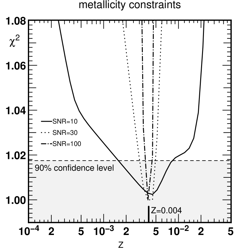
Figure 15: The high resolution spectral energy distribution of model extinctionless mono-metallic population with $Z=0.004$ is inverted using spectral bases with different metallicities for several SNR. For $\mathrm{SNR}=10$ per pixel, the metallicity is moderately well constrained ($\Delta Z\approx 1\;\mathrm{dex}$), while for $\mathrm{SNR}\geq 30$ per pixel all the metallicities other than $0.004$ can be rejected at the $90\%$ confidence level.

When attempting to reconstruct the stellar age distribution from real observations, one would still have to guess the metallicity of the population. A classical parametric way to proceed would be to perform a mono-metallic inversion for each of the available metallicities in the basis. If the dominant observational error is Gaussian, we expect the $\chi^{2}$ to be minimum when using the true metallicity. However, because of the age-metallicity degeneracy, it might not be so clear, and one could expect to reach a good $\chi^{2}$ even with an erroneous metallicity guess, resulting in an error in age estimation. Figure 15 shows a plot of the reduced $\chi^{2}$ when inverting a population of metallicity $Z=0.004$ with a basis of different metallicity for several SNR and $R=10\,000$. The smoothing parameter was chosen using GCV with the $Z=0.004$ kernel. The best fit is always obtained when the initial model metallicity is used. We computed the $90\%$ confidence level by taking as the number of degrees of freedom, the number of pixels in the spectrum minus the number of age bins ($40$ in this example). This choice could be discussed because the weights of adjacent time bins are correlated by the penalization. However, the number of time bins remains far smaller than the number of pixels and thus plays no critical role. For $\mathrm{SNR}=10$ per pixel (i.e. $\mathrm{SNR}=20$ per Å), we can not reject fits with wrong metallicities $Z\in[0.002,0.009]$. The error on metallicity can therefore reach $0.35\;\mathrm{dex}$ for $\mathrm{SNR}=10$. The range of acceptable metallicities however shrinks rapidly with increasing SNR, tightening the constraints. At $\mathrm{SNR}\geq 30$, it is possible to break the age-metallicity degeneracy, and thus to let metallicity be a free parameter of the inversion problem.

This closes our detailed investigation of the idealized problem of recovering the stellar age distribution of a mono-metallic, reddening-free stellar population.

5 Stellar content and reddening recovery

The previous section presented STECMAP in an idealized regime, which could only be applied to observations where both the metallicity and the extinction are known a priori, which is rarely the case in reality. We now present an extension of STECMAP accounting for these additional free parameters as well. In Sect. 5.1, the full linear age-metallicity problem is examined, where both metallicity mixing and age mixing are allowed, and study its behaviour. Then, for simplicity, and given the extremely poor conditioning of this problem, the unknown metallicity will be handled specifically as an age-metallicity relation. The technique for reconstructing the stellar age distribution, the age-metallicity relation and the extinction will be presented in Sect. 5.2, along with a few example simulations in Sect. 5.3, and finally its applicability and accuracy will be discussed while exploring several observational regimes in Sect. 5.4.

5.1 2D Linear age-metallicity problem

Here we consider a very composite population where several sub-populations with different ages and metallicities are superimposed. Let us define a $2$D stellar age and metallicity distribution $\Lambda(t,Z)$ yielding the fraction of optical flux emitted by stars with age $t\in[t,t+\mathrm{d}t]$ and metallicity $Z\in[Z,Z+\mathrm{d}Z]$. The model spectrum is the integral of $\Lambda$ over age and metallicity space. Discretizing as in Sect. 3, we get the discrete model spectrum as the weighted sum of the single stellar populations for all the ages and all the metallicities in the basis. Here the parameter vector is a $2$D map containing the weights $x_{ij}$ of the single stellar population of age $t_{i}$ and metallicity $Z_{j}$. The model matrix $\mathbf{B}$ is the concatenation of the mono-metallic bases described in Sect. 3, i.e. sequences of single stellar populations in age and metallicity. Its conditioning number is commonly of order $10^{8}$, telling us that thorough regularization is required.

5.1.1 Where is the information on $Z$?

In a manner similar to Sect. 3.7 we can determine which spectral domains are important for age and metallicity determination. We compute the inverse model matrix $\tilde{\mathbf{B}}$ of the problem for a given $\mathrm{SNR_{d}}$ and look for large peak to peak variations in this matrix, indicating spectral features having strong discriminative power, as shown in Fig. 16. Most of the bands involved in the Lick indices carry a lot of information. However, some of them, like TiO₂, seem to be unimportant, and a large number of medium and high resolution lines not involved in Lick indices actually carry most of the information.The comparison with Fig. 6 shows that several metallic lines, which were not important for a mono-metallic population age distribution recovery, turn out to carry a substantial part of the information when the metallicity is unknown. Again, the blue part of the spectrum seems to be more discriminative.

Since age sensitive and metallicity sensitive lines are spread along the whole optical wavelength range, any small section of the spectrum has good chances of containing such lines (see Le Borgne et al. (2004) for an example around H_γ). Thus, if the available data does not allow reliable full optical domain fitting, plots such as Fig. 16 are a good starting point for the search for new high resolution indices. The use of the whole spectrum implies some redundancy, but considering the sensitivity of the inversion problem to noise, this redundancy is highly welcome.

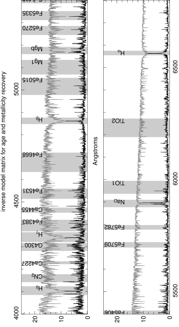
Figure 16: Same as in Fig. 6 for the linear age-metallicity distribution recovery. The dimensions of the inverse problem are $60$ age bins and $5$ metallicity bins. The smoothing parameter is set by GCV for $\mathrm{SNR}=100$ per pixel. The grey solid line is a $1$ Gyr half-solar metallicity single stellar population for reference. Many of the spectral domains involved in the definition of the Lick indices system seem to carry more information than the rest of the spectrum. However, the information is still widely spread along the whole optical range in the form of medium depth lines, suggesting there is a large number of potential high resolution indices.

5.1.2 Age-metallicity degeneracy?

We carried out the following experiment illustrated in figure 17. We produced mock data corresponding to a $2$D stellar age and metallicity distribution map $\mathbf{x}$ and investigated how well we could reconstruct it for a given SNR. In the example of figure 17 (top panels), the model is a mono-metallic bump centered on $1$ Gyr and $Z=0.008$. The corresponding mock data is noised and then inverted as in Eq. (31) except that $\mathbf{B}$ is now the multi-metallic single stellar population basis defined above. The penalization is Laplacian. In this experiment, we focus on the broadening of the bump in the metallicity direction as a signature of the age-metallicity degeneracy.

The inspection of the first non attenuated solution singular modes tells us about the properties of the regularized problem. The panels c and d of Fig. 17 show the second and the fifth solution singular modes of the model matrix $\mathbf{B}$. Each of them is an age-metallicity map. The shapes of the stellar age distribution for each metallicity in the second singular mode are very similar, indicating bad separability between metallicities. Thus, if only the first singular modes are recovered, the solutions will have a strong tendancy to be flat in the metallicity direction.

The fifth singular mode is the first one to show a well-defined structure: a bump in age, elongated in the metallicity direction, with a slight shift to larger ages with decreasing metallicities. This traces the age-metallicity degeneracy: a pure mono-metallic population will be reconstructed in regularized regimes as a composite, mixing younger metal rich single stellar populations with older metal poor single stellar populations. The a and b panels of Fig. 17 show reconstructions of such age-metallicity maps for $R=10\,000$, $\mathrm{SNR}=500$ and $200$ per pixel. The model consists of a single bump centered on $1$ Gyr and $Z=0.008$, and the penalization is Laplacian. For $\mathrm{SNR}=500$ per pixel we see that the population is effectively reconstructed as a single bump in age and metallicity. The age-metallicity degeneracy is in this example explicitly broken. The same experiment with $\mathrm{SNR}=200$ per pixel gives a solution degenerate in metallicity: the mono-metallic population is seen as the sum of three mono-metallic sub-populations contributing nearly equally to the total light. The younger component is more metal-rich, while the older one is poorer, as is expected for age-metallicity degenerate solutions, and is similar to the trend seen in the solution singular modes. In this example, the smoothing parameter was chosen by generalized cross validation. More realizations of this experiment gave similar degenerate solutions. From the shape of the fifth solution singular mode, we can measure the slope of the age-metallicity degeneracy, that is the slope defined by the maxima of the bumps of the singular mode in the age-metallicity plane. We find it to be equal to $0.3$, which is much smaller than the $3/2$ given in Worthey (1994). Smaller slopes indicate a better definition of age. This is expected because here we consider the whole optical range and the continuum as reliable.

As a conclusion, we found $2$D age-metallicity map reconstructions to be feasible for only very high ${\mathrm{SNR}}\geq 500$. Since this is comparable or larger than $\mathrm{SNR_{b}}$, we consider it strongly unphysical. Moreover, from an observational point of view, such a high $(\mathrm{SNR},R)$ combination for an outer galaxy is generally unreachable in reasonable time with the present generation of instruments. Thus, inversions with this complexity and SNR are doubly challenging. We now address a simplified version of this problem by reducing the metallicity parameters to a $1$D age-metallicity relation.

Figure 17: (a) and (b): Free metallicity reconstructions of a mono-metallic population for $\mathrm{SNR}=500$ and $\mathrm{SNR}=200$ per pixel. For high $\mathrm{SNR}$ a mono-metallic population is unambiguously recovered, while at lower SNR, a multi-metallic solution appears, indicating the degeneracy of the problem. (c) and (d): solution singular modes of the $2$D age-metallicity reconstruction problem. The difficulty involved in such a reconstruction arises from the very bad conditioning number, and the lack of features of the first singular modes in the metallicity direction.

5.2 Non-linear age-metallicity recovery

In the rest of the paper we assume that the chemical properties of the population are represented by an age-metallicity relation $Z(t)$ of unknown shape. In contrast to Sect. 5.1, the sub-population of age $t_{j}$ is therefore assigned one and only one metallicity $Z_{j}$ rather than a metallicity distribution. In addition, we now allow the spectral energy distribution to be affected by an extinction $f_{\mathrm{ext}}(E,\lambda)$ parameterized by the color excess $E$. Finally, accounting for the age distribution $\Lambda(t)$, the observed spectral energy distribution at rest then writes:

$$F_{\mathrm{rest}}(\lambda)=f_{\mathrm{ext}}(E,\lambda)\,\int_{t_{\mathrm{min}}}^{t_{\mathrm{max}}}\Lambda(t)\,B\bigl{(}\lambda,t,Z(t)\bigr{)}\,\mathrm{d}t\,.$$ (38)

This model is linear in age distribution $\Lambda$, and non linear in metallicity $Z$ and extinction $E$. Recall that $f_{\mathrm{ext}}$ may be replaced by other parametric functions of wavelength that could for instance describe flux calibration corrections.

5.2.1 Discretization and parameters

Following the same prescription as in Sect. 3, but accounting for extinction, we can derive the discretized version of Eq. (38). Provided the extinction law is very smooth compared to the size of the wavelength bins, the model of the sampled spectral energy distribution of the reddened composite stellar population in the $i$-th spectral bin writes:

$$s_{i} = \int F_{\mathrm{rest}}(\lambda)\,g_{i}(\lambda)\,\mathrm{d}\lambda$$ (39)

$$\approxeq f_{\mathrm{ext}}(E,\lambda_{i})\!\int\!g_{i}(\lambda)\!\int_{t_{\mathrm{min}}}^{t_{\mathrm{max}}}\!\!\Lambda(t)\,B\bigl{(}\lambda,t,Z(t)\bigr{)}\,\mathrm{d}t\,\mathrm{d}\lambda,$$

which simplifies to:

$$s_{i}=f_{\mathrm{ext}}(E,\lambda_{i})\,\sum_{j=1}^{n}B_{i,j}\,x_{j}\,,\quad i\in\{1,..,m\}\,,$$ (40)

or in matrix form:

$$\mathbf{s}=\operatorname{diag}\bigl{(}\mathbf{f}_{\mathrm{ext}}(E)\bigr{)}\cdot\mathbf{B}\cdot\mathbf{x}\,,$$ (41)

where the kernel matrix $\mathbf{B}$ and the vector $\mathbf{x}$ of the age distribution $\Lambda(t)$ sampled upon time are defined as in Sect. 3, and $\operatorname{diag}(\mathbf{f}_{\mathrm{ext}})$ is the diagonal matrix formed from the extinction vector:

$$\mathbf{f}_{\mathrm{ext}}(E)=\bigl{(}f_{\mathrm{ext}}(E,\lambda_{1}),\ldots,f_{\mathrm{ext}}(E,\lambda_{m})\bigr{)}^{\top}\,.$$ (42)

which contains the extinction law seen by the population and depends non-linearly on the color excess ${E}$. Note that $\mathbf{B}$ contains the single stellar population basis for the age-metallicity relation vector $\mathbf{Z}$ (the age-metallicity relation $Z(t)$ sampled in time).

From a computational point of view, any matrix product involving $\operatorname{diag}\bigl{(}\mathbf{f}_{\mathrm{ext}}(E)\bigr{)}$ is very expensive and can be profitably implemented using term to term product. However, in order to save the introduction of confusing operators, we will carry on with the current notation.

5.2.2 Smoothness a priori with MAP

The model defined by Eq. (41) is non-linear because of the dependancies of $\mathbf{T}$ and $\mathbf{B}$ on respectively $E$ and $\mathbf{Z}$. We can therefore not refer to the classical definition of ill-conditioning. However, since the simpler problem solved in Sect. 3 is ill-conditioned, it is expected that the more complex problem treated here will be even more ill-conditioned, all the more since we now seek two fields plus one extinction parameter. We will thus add a priori information by implementing smoothness constraints, and allow the unknowns to have different smoothing parameters. We define the penalizing function $P_{\mathrm{smooth}}$ by

$$P_{\mathrm{smooth}}(\mathbf{x,Z})\equiv\mu_{\mathbf{x}}P(\mathbf{x})+\mu_{\mathbf{Z}}P(\mathbf{Z})\,,$$ (43)

where $P$ is the standard quadratic function defined by (29).

5.2.3 Metallicity bounds

The metallicity range $[{Z_{\mathrm{min}}},{Z_{\mathrm{max}}}]$ for which models are available is bounded. We must therefore find a way to ensure that the solution lies in the desired metallicity range by making unwanted values of $Z$ unattractive. To do this we use a binding function $c$ ($c$ stands for constraint) which is another kind of penalizing function. This technique was proposed by R. Lane (private communication). The function $c$ must be flat inside $[{Z_{\mathrm{min}}},{Z_{\mathrm{max}}}]$ in order not to influence the metallicity search and increase gradually outside. We define $c$ piecewise by

$$c(Z)=\quad\left\{\begin{array}[]{ll}(Z-{Z_{\mathrm{min}}})^{2}&\mbox{if }Z\leq{Z_{\mathrm{min}}}\,,\\ (Z-{Z_{\mathrm{max}}})^{2}&\mbox{if }Z\geq{Z_{\mathrm{max}}}\,,\\ 0&\mbox{else}\,.\end{array}\right.$$ (44)

The binding function $C$ used in practice is defined by

$$C(\mathbf{Z})=\sum_{j}c(Z_{j})\,.$$ (45)

The penalization function we finally adopt is

$$P_{\mu}(\mathbf{x},\mathbf{Z})\equiv P_{\mathrm{smooth}}(\mathbf{x},\mathbf{Z})+\mu_{C}\,C(\mathbf{Z})\,,$$ (46)

where a binding parameter $\mu_{C}$ allows to set the repulsiveness of the exterior of $[{Z_{\mathrm{min}}},{Z_{\mathrm{max}}}]$. The objective function,

$$Q_{\mu}=\chi^{2}(\mathbf{s}(\mathbf{x},\mathbf{Z},E))+P_{\mu}(\mathbf{x},\mathbf{Z})\,,$$

is now fully characterized. Its derivatives are given in the appendix B.

5.3 Simulations of metal dependent LWSAD

We applied the proposed inversion method to mock data for various stellar age distributions, age-metallicity relations, extinctions and SNR. In this case, choosing an input model involves choosing the functions $\Lambda(t)$, $Z(t)$, and a color excess $E$. The corresponding model spectrum is then computed following (41). Gaussian noise is added to obtain the pseudo-data.

Figure 18 shows simulations of reconstructions in the case of high quality pseudo-data: $R=10\,000$ at $4000-6800$ Å with $\mathrm{SNR}=100$ per pixel for $100$ realizations. The left panels show the stellar age distribution while the right panels show the age-metallicity relations. The top row shows reconstructions of a double-burst population where the two bursts have different luminous contributions. The young component accounts for $75\%$ of the light, and its metallicity is a tenth of the old component’s, which contributes only to $25\%$ of the total light. The unbalance between the young and old luminous contributions should make it more difficult to constrain the old component. Still, the reconstructions are good in the sense that the bumps are properly centered and scaled. Metallicities are also adequately recovered. The reconstructed stellar age distributions are smoothed versions of the model, as expected.

The bottom line plots illustrate the case of a continuous rather than bumpy stellar age distribution. All ages contribute equally to the light except the youngest and oldest ones. The model age-metallicity relation yields a metallicity $Z(t)$ that increases with time. The rise and decay of the recovered age distribution are adequately located, and the metallicities have the correct trend. The metallicities of the youngest component are unconstrained simply because they do not contribute to the total light.

For each realization of these simulations, the color excess was a random number between $0$ and $1$. In each case, it was recovered with an accuracy better than $10^{-2}$.

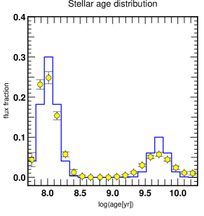
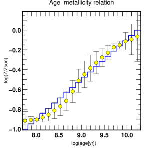
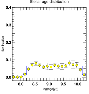
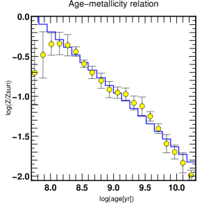
Figure 18: Reconstruction of the stellar age distribution (left) and age-metallicity relation (right) for $R=10\,000$ and $\mathrm{SNR}=100$ per pixel. The thick line is the input model. The circles and the bars show respectively the median and the interquartiles of the recovered solutions for 100 realizations. The metallicities and flux fractions of the populations with significant contributions are adequately recovered. In each experiment, the extinction parameter of the model was chosen randomly and recovered with good accuracy.

5.4 Age separation of metal dependent LWSAD

In a realistic observationnal setting, we would like to age-date superimposed populations. For such investigations, it is essential to have a good understanding of the limitations of the non-parametric method. We therefore investigated again how well we could reconstruct two superimposed bursts of unknown metallicities and extinction. We proceeded as in Sect. 4.2, and the grid of double burst ages is the same. Both bursts contribute equally to the total light. In a first set of experiments, the model age-metallicity relation is arbitrarily chosen as $\log(Z)=-9.95+0.85\,$ log(age[yr]), where the age ranges from $50$ Myr to $15$ Gyr. It is not supposed to be a physically motivated choice, but allows us to explore about $2$ decades in metallicity. The allowed range for the solution age-metallicity relation is $[{Z_{\mathrm{min}}}=0.0004,{Z_{\mathrm{max}}}=0.05]$. The extinction parameter was chosen randomly between $0$ and $0.5$. The reconstructions were performed without any a priori for the age-metallicity relation, stellar age distribution or extinction parameter, apart from the requirement of smoothness. For each pseudo-observational context, the smoothing parameter was set using the GCV value for the mono-metallic case and fine-tuned for a small separation between 2 bursts. The smoothing parameter for the age-metallicity relation was set to a large value (around $10^{3}$) because we just wish to recover a global trend of the metallicity evolution in the reconstruction. A flat guess for all variables was the starting point. In every case we converged to a stable solution in less than $1500$ iterations, corresponding to $\approx 1$ minute on a $1$ Ghz pc for a $R=10000$ basis (i.e. $14000$ pixels of $0.2$ Å) with $60$ age bins. The distribution of the reduced $\chi^{2}$ of the solutions were found to follow a Gaussian distribution law with unit mean, showing that each experiment had properly converged.

We are thus able to give an estimate of the resolution in age versus SNR and spectral resolution. Figure 19 shows some of the results of our simulation campaign. On each panel we plotted the results obtained at $R=2\,500$ (upper octan) and $R=10\,000$ (lower octan). The results for $R=1\,000$ and R=$6000$ are very similar and are not shown. The number of successful inversions rises with increasing SNR, and the unseparable zone in the diagram shrinks. In the same way, the error bars and bias reduce with increasing SNR. We give the resolution in age for several SNR per Å and spectral resolutions in Fig. 20. It improves with increasing SNR, but settles around $0.8\;\mathrm{dex}$ for very high quality data. The variation of the resolution in age with spectral resolution is not significant compared to the statistical error ($\approx 0.25\;\mathrm{dex}$), so that no trend with spectral resolution can clearly be deduced. The middle panel shows the median error on the luminous weighted ages of the two bursts for the successful separations. The error decreases with increasing SNR down to $0.02\;\mathrm{dex}$ for $\mathrm{SNR}=200$ per Å, and is significantly lower for the high resolution experiments (the relative statistical error for this measure is smaller than $5\%$). We see the same trend in the metallicities median errors of the double bursts, in the right panel. The smallest error is obtained for the highest spectral resolution. The general smallness of these errors is partly explained by the severity of the selection, that rejects as non separable any ambiguous solution.

Somewhat unexpectedly, the results do not depend on the slope of the age-metallicity relation adopted for the double-burst models. With a negative slope, a young metal-rich population is added to an old metal-poor one. In view of the age-metallicity degeneracy, this should be the least favorable situation for a proper separation. We performed simulations with positive and negative slopes and obtained identical results considering the statistical errors given above. Thus, the age-metallicity degeneracy is not a limiting factor in our experiment.

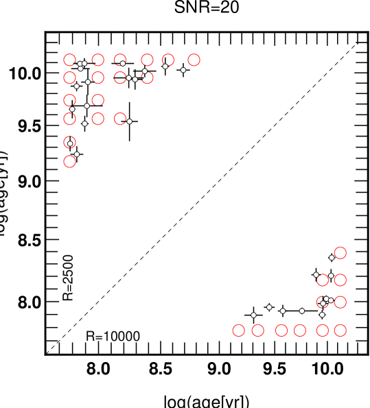
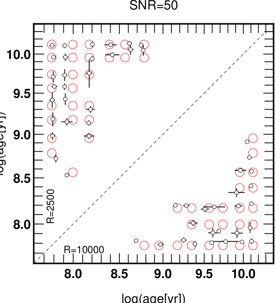
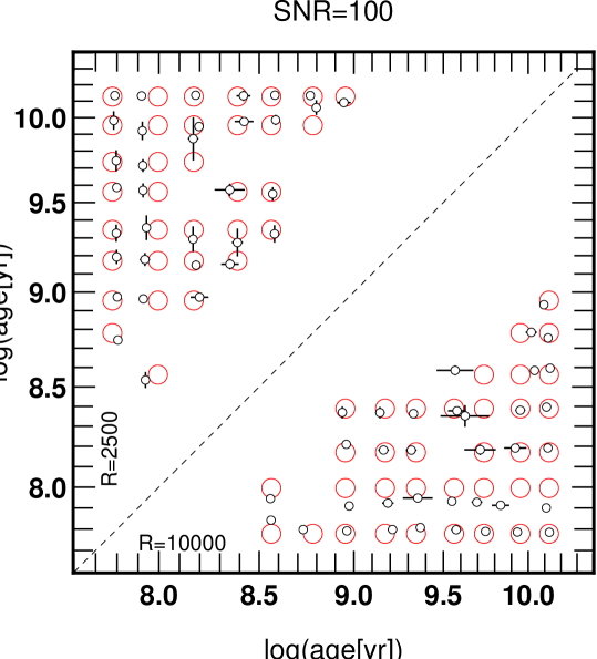
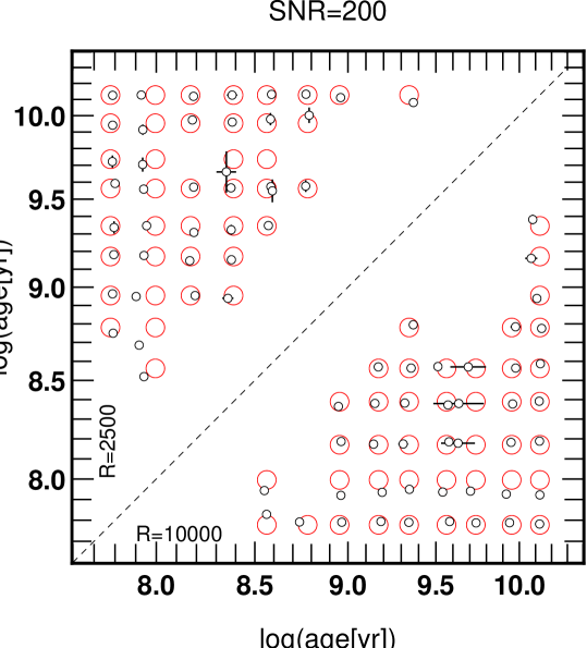
Figure 19: Same as Fig. 12 but the metallicities and the extinction are free parameters. The SNR is given per Å. The ability to separate close sub-populations improves with SNR, as does the accuracy of the age estimates.

Figure 20: Left:Resolution in age [dex] versus SNR per Å for various spectral resolutions. As expected, the resolution in age improves with increasing SNR. It settles around $0.8\;\mathrm{dex}$ for the highest SNR. No significant trend is seen with spectral resolution. Middle: Median error on the age of the bursts [dex] in the successful separations vs SNR for several resolutions. High resolution experiments give the smallest errors. Right: Same as middle panel but for metallicity estimates. Again, the best accurracy is obtained at high spectral resolution, given the same total number of photons.

6 Conclusions and prospects

Let us sum up our findings relative to the diagnosis of the linear (mono-metallic) problem (Sect. 3 and 4) and the more realistic non linear problem of recovering simultaneously the luminosity weighted stellar age distribution, the extinction and the age-metallicity relation  (Sect. 5) in turn, and close on the observational and methodological prospects of STECMAP.

6.1 Probing the linear problem: the tricks of the trade

The idealized problem of recovering the non-parametric stellar age distribution of a mono-metallic population seen without extinction is linear. The conditioning number of the kernel is very large and accounts for the ill conditioning of the problem, i.e. pathological sensitivity to noise in the data.

The noise in the single stellar population models also limits the number of free parameters that may be recovered robustly to describe the star formation history. In textbook inversion problems, this number can be estimated quantitatively from the sequence of singular values of the single stellar population basis. Here however, this theoretical value is misleading because the expected signature of the model noise in the singular value spectrum is not apparent. We explained this by the correlations between the noise patterns in subsequent basis spectra. To obtain the number of free parameters, the singular values are used together with an independent estimate of the SNR of the basis. For the optical spectral range covered with Pegase-HR and ages ranging from $50$ Myr to $15$ Gyr, the corresponding number is 6. This makes high frequency variations of the stellar age distribution unrecoverable, no matter the data quality, $\mathrm{SNR}_{\mathrm{d}}$, and the inversion method.

When the dominant error source is the data, the problem may be regularized by truncating the singular value decomposition  or reducing the number of age bins so that $\sigma_{1}/\sigma_{n}\leq\mathrm{SNR_{d}}\sqrt{m}$. This crude rule can be used to obtain a quick estimate of the performance expected for a given dataset.

The problem can be more profitably regularized without reducing arbitrarily the number of age bins by imposing the smoothness of the solution, to obtain a penalized likelihood estimate. This constraint reduces the risk of overinterpreting the data. The smoothing parameter is set automatically by generalized cross validation for each ${\mathrm{SNR_{d}}}$, or/and by performing simulations in a suited pseudo-observational context.

For an adequately regularized problem, we defined the inverse model matrix and inspected it in order to find the wavelength ranges which are most discriminative for age determinations. We found that the information is widely distributed along the optical range (cf. Figs. 6 and 16).

The behaviour of the inversion can be predicted by inspecting the singular value decomposition or generalized singular value decomposition of the kernel. The first non-attenuated solution vectors are responsible for the detailed shape of the regularized reconstructions, and thus for the generation of artifacts. The general shape of the solution vectors, and especially the presence/absence and location of their oscillations, gives an indication in which age ranges the inversion behaves worst.

In particular, the inspection of the SVD components revealed that the problem of recovering flux distributions was less pathological than the problem of recovering mass fractions. More specifically, the transition rank $i_{0}$ between signal and noise dominated regimes is independent from the fiducial model in the recovery of flux fractions.

Second or third order penalizations gave similarly good results, showing that the quality of the inversion does not rely strongly on the details of the regularization.

Requiring the solutions to be positive improves the results even further, and in particular reduces Gibbs ringing, as can be seen by comparing Fig. 8 and Fig. 10.

One should be aware that the efficiency of the inverse method cannot be assessed on the basis of a small set of simulations. Indeed, it is easy to produce good looking results down to ${\mathrm{SNR_{d}}}=0.1$ per pixel by carefully choosing the model age distribution.

We performed an extensive simulation campaign by inverting a grid of double burst models in several pseudo-observational regimes. If the age difference between the bursts is larger than $0.4\;\mathrm{dex}$, we were able to separate the $2$ components and recover their ages with a very small error from high quality data ($\mathrm{SNR_{d}}=200$ per Å).

However, the high $\mathrm{SNR_{d}}$ regime for which we obtained the best results are questionable. Indeed, when ${\mathrm{SNR_{d}}}$ and ${\mathrm{SNR_{b}}}$ are comparable, the number of degrees of freedom is imposed by the noise in the basis rather than in the data. We therefore consider the extreme regimes with ${\mathrm{SNR_{d}}}\geq 200$ per Å unphysical: small oddities (of uncertain nature) in the basis are seen as physically discriminative information. Only an improvement of $\mathrm{SNR_{b}}$ could in principle increase the number of degrees of freedom. Assuming that the singular values spectrum of the initial kernel shown in Fig. 4 is representative of the basis even at higher $\mathrm{SNR_{b}}$, we can set the following rules of thumb.

1. If for example $\mathrm{SNR_{d}}=100$ per pixel, the maximum number of freedom degrees one may consider is of order $8$ ($n=8$ from criterion (25) or Fig. 2).

2. To ensure that no serious contamination of the singular values by noise in the basis happens for $i<8$, one would need $\mathrm{SNR_{b}}\geq 1\,000$ per pixel (estimated from Fig. 4) ($2\,500$ per Å). We caution that this is an extrapolation, and that the actual behaviour of single stellar population spectra at this kind of SNR is not known.

By comparing the solutions given by singular value decomposition and the Gram-Schmidt othonormalized kernel we showed that ill-conditioning remains an issue when working with compressed data.

Finally, the mismatch observed when a mono-metallic population is fitted by a basis of different metallicity allowed us to constrain this additional metallicity parameter with a $\mathrm{SNR_{d}}$ as small as $10$ per pixel, well enough to motivate a feasibility study of the recovery of the age distribution, the metallicities and the reddening of a composite stellar population.

6.2 Beyond the mono-metallic inversion?

The ill-conditioned problem of recovering a $2$D age-metallicity distribution of a composite unreddened population can also be recast into a linear problem. A penalized likelihood estimate can be obtained by means of additionnal smoothness constraints. The inspection of the regularized inverse model matrix reveals that a large number of age and metallicity sensitive lines carrying discriminative information are located all along the optical range. The shape of the first solution singular modes shows that age-metallicity degenerate solutions are expected even for $\mathrm{SNR_{d}}$ as large as $200$ per pixel. Notwithstanding the above caveat about high SNR, the inversions with such a complexity are thus unfeasible in realistic regimes from optical integrated light only.

A natural simplification involves assuming that the metallicity of the population can be described by a one to one non parametric age-metallicity relation. The problem of recovering the stellar age distribution, the age-metallicity relation and an extiction parameter then becomes tractable provided that adequate regularization (smoothness, bound and positivity) is implemented, and yields a penalized likelihood estimate.

A detailed simulation campaign allowed us to estimate the resolution in age that can be achieved from optical data in several pseudo-observational regimes. If the time elapsed between $2$ instantaneous bursts is larger than $0.8\;\mathrm{dex}$, they can be separated unambiguously by STECMAP from high quality data ($\mathrm{SNR_{d}}=100$ per Å), and their ages and metallicities can be constrained with an accuracy of respectively $0.02\;\mathrm{dex}$ and $0.04\;\mathrm{dex}$. In such regimes, the age-metallicity degeneracy is effectively broken. For smaller separation, there is always a mono-burst or smoother solution that fits the data equally well. Our experiments reveal no clear dependency of the resolution in age on the spectral resolution $R$ ($\geq 1\,000$) as long as the SNR per Å (or integration time) is conserved in the comparative experiments. As in the preliminary conclusion for the idealized mono-metallic unreddened problem, it is not clear whether the extreme $\mathrm{SNR}_{\mathrm{d}}$ are physical or not, since in these regimes the noise in the basis is not negligible any more compared to the noise in the data. In any case, $0.8\;\mathrm{dex}$ should be considered as a lower resolution limit, for any separation attempt in the range $\lambda\lambda=[4\,000\;\mbox{\AA},6\,800\;\mbox{\AA}]$.

The fact that free extinction does not hinder the inversions indicates that the continuum is not a critical constraint. Simulations with more complex corrections on the continuum (not described in this paper) confirm this point. The information on age and metallicities is carried in the line spectrum.

6.3 Discussion and prospective

Perhaps the most intriguing conclusions of this paper are the small number of degrees of freedom found in an optical single stellar population basis even with $\mathrm{SNR_{b}}$ as large as Pégase-HR, and the very anti-intuitive hint that significantly larger SNR is needed in the basis than in the data to be analyzed. It highlights the need to study and quantify the influence of the models noise in linear and non-linear inversions, and to continue and improve the various steps involved in the construction of the model.

Several directions can be followed, on the basis of Sect. 2.3. Empirical libraries should improve with the combination of large collecting areas, and high resolution, large coverage instruments with massive multi object capacities, which should boost up the construction of libraries by a significant factor. The library UVES POP (Bagnulo et al., 2003) is an example. With telescopes of the 10m class or larger, stars in clusters and in Local Group galaxies can be observed to remedy in part the issue of completeness and some of the biases of solar neighbourhood libraries (e.g. more luminous metal-poor stars, or stars with modified $\alpha$-element abundances).

On the theoretical side, one should investigate accurately and systematically what drives the shape of the singular value spectrum of the SSP basis. In this paper we concentrated on a given SSP model, without tuning the basis to study the effect of e.g. sampling strategies on the conditioning. Since the behaviour of an inverse problem depends on the shape of the solution singular vectors as well, it is a key issue to understand what drives their shape. Making them smoother and more regular is a step towards reducing the generation of artifacts. Clearly, one would want to question the sampling strategy in $(T,g,Z)$ space in terms of both the conditioning number of $\mathbf{B}$ and the roughness of its singular vectors. In particular, one would like for instance to apply an error weighted regularized tomographic interpolation in $(T,g,Z)$ space, in order to construct a noise free spectral basis, which would by construction prevent from interpolating the noise from one spectrum to another. Even though the interpolation of the noise patterns of individual stars in the library may explain the vanishing of the saturation of the singular values, we still miss a quantitative relation between the density of library stars in $(T,g,Z)$ space, their SNR, and the slope of the singular value spectrum.

Ultimately one should aim at designing inverse methods where the errors in the models are explicitly taken into account (for instance using TLS) in order to draw a consistent error budget.

The generally very limited separability of successive star formation episodes in most pseudo-observational settings is in strong contrast with the results of a number of more optimistic authors. In particular, if one is bound to draw cosmological constraints from the stacking of a large set of noisy star formation histories, it is still essential to check that individual star formation histories are well recovered, since otherwise the median solution is likely to be dominated by artifacts. Exhaustive testing of the method as we propose is in this case a mandatory step.

The spectral energy distribution matching procedures and parameter recovery presented here are absolutely not model-dependent and could be used in association with any other stellar population model as is. It will thus be interesting and informative to perform the same kind of study (resolution in age, conditioning) with other existing evolutionary synthesis models, in order to quantify the amount of information and the constraints to be expected from observations in other wavelength domains, as the UV, NIR or FIR. It is expected that increasing the wavelength coverage should improve significantly the resolution in age and the behaviour of the problem in general. The possible discrepancies between the models are also a major matter of concern. For instance, are the metallicity constraints using a given set of single stellar populations robust to a change of the evolutionary synthesis code? It will be interesting to test this by producing mock data with one available code (Bruzual & Charlot, 2003; Gonzalez Delgado et al., 2005) and interpreting them with another one. We expect misfits to arise from wavelength calibration error, small scale flux calibration errors, and systematic deviations caused by the use of different evolutive tracks, IMFs, and stellar libraries. This exercise will allow us to investigate the amount of error introduced by the models themselves.

The methods we described together with the corresponding error and separability analysis will be very useful for interpreting large sets of data from large surveys such as SDSS, 2DFGRS, DEEP2, $\cdots$, and also for upcoming new generation instruments, especially high resolution instruments with multi-object or field integral capacities, for instance FALCON (Puech & Sayede, 2004), or MUSE (Henault et al., 2003). In this context, astronomers will want to extract kinematical information as well, and question the relationship between the kinematics and the nature of the stellar populations. The simultaneous recovery of the kinematical distribution and the corresponding stellar population via the non-parametric interpretation of spectra is described in a companion paper.

Appendix A Dependence of the signal-noise transition on the fiducial model

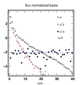
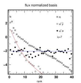
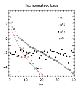
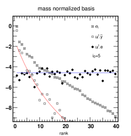
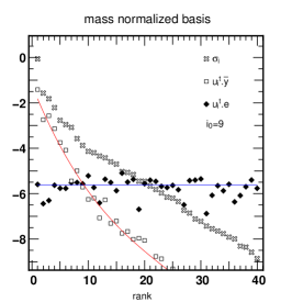
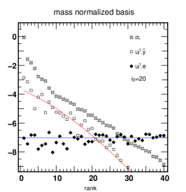
Figure 21: Study of the location of the signal-noise transition rank as a function of the fiducial model. The figures are the same as Fig. 2, with the same pseudo-observational setting (SNR=100 per pixel), for a flux-normalized (top) and a mass-normalized basis (middle) respectively, for 3 different fiducial models $\overline{\mathbf{x}}$, given at the bottom of each column. Polynomial fits are given for the signal and noise singular coefficients. The transition rank $i_{0}$ is given in each figure as the intersection of these fits. For the mass-normalized basis, the rank of the transition between signal and noise dominated regimes spans a wide range of values depending on the fiducial model $\overline{\mathbf{x}}$. On the contrary, for the flux-normalized basis, the transition rank is rather constant with regard to modifications of the age of the fiducial model.

In this section we clarify the relation between the transition rank $i_{0}$ between the noise and signal dominated regimes (the intersection of the $\mathbf{u}_{i}^{\top}\cdot\overline{\mathbf{y}}$ with the $\mathbf{u}_{i}^{\top}\cdot\mathbf{e}$) and the fiducial model, as defined in Sect. 3.4 and Fig. 2. More specifically, we explore the shift of the transition by varying the age of the fiducial model, for a flux-normalized and a mass-normalized basis. The results are shown in Fig. 21. The fiducial models are given in the bottom of each column. Note that the $y$ axis is labeled “flux fractions” on the left and “mass fractions” on the right. This is to recall that the interpretation of the model curve differs, depending on the adopted normalization of the basis. Compared to Fig. 2, we added a 3rd order polynomial fit to the signal singular coefficients and a constant fit to the noise coefficients. This allows to detect automatically and objectively the transition rank $i_{0}$, as the intersection of the two fits.

For the mass-normalized basis, the transition moves from the 5-th rank (for the youngest fiducial model) up to the 20-th (for the oldest fiducial model). On the other hand, the location of the transition for the flux-normalized basis is rather unaffected by changes of the fiducial model and remains around rank 7-9.

Appendix B Gradients of $Q_{\mu}$

The direct linear solution which minimizes the objective function $Q_{\mu}$ can only be used in the case of a linear model (with respect to the parameters) and without constraints (such as positivity). For all other cases, the objective function $Q_{\mu}$ can only be minimized by means of an iterative method. The most efficient and yet simple to use of these methods require the computation of the objective function and of its gradient. These optimization methods are: the conjugate gradients and variable metric methods (e.g. BFGS). In practice for non-linear problems, variable metric methods have been found to require less iterations and less function evaluations than conjugate gradient ones (Thiébaut, 2002). For that reason, we used the limited memory variable metric method VMLM-B implemented in the OptimPack package written by E. Thiébaut for Yorick (http://www.maumae.net/yorick/doc/index.html).

Since the efficiency of these iterative optimization algorithm rely on the correctness of the gradient of $Q_{\mu}$ (i.e. partial derivatives of $Q_{\mu}$ with respect to the free parameters), we devote this appendix to the derivation of such partial derivatives for the different cases considered in this paper. Whenever it was possible (i.e. in the linear case), the iterative solutions were tested against the analytical solutions, and were found to be identical down to machine precision.

B.1 Simple Linear Model

In the linear problem, the gradients of $Q_{\mu}$ have simple expressions:

$$\frac{\partial\chi^{2}}{\partial\mathbf{x}} = -2\,\mathbf{B}^{\top}\cdot\mathbf{W}\cdot\left(\mathbf{y}-\mathbf{B}\cdot\mathbf{x}\right)\,,$$ (47)

$$\frac{\partial P}{\partial\mathbf{x}} = 2\,\mathbf{L}^{\top}\cdot\mathbf{L}\cdot\mathbf{x}\,.$$ (48)

B.2 Age-Metallicity-Extinction Gradients

For the resolution of the age-metallicity-extinction problem (Sect. 5), the objective function $Q_{\mu}$ is a $\chi^{2}$ penalized by regularization terms and a binding function. The regularization terms being the same as in the linear case, their gradients are given by Eq. (48). The gradient of the binding function $C$ for a metallicity vector $\mathbf{Z}$ reads:

$$\left(\frac{\partial C}{\partial\mathbf{Z}}\right)_{j}=\left\{\begin{array}[]{ll}2\,(Z_{j}-{Z_{\mathrm{min}}})&\mbox{for }Z_{j}<{Z_{\mathrm{min}}}\,,\\ 2\,(Z_{j}-{Z_{\mathrm{max}}})&\mbox{for }Z_{j}>{Z_{\mathrm{max}}}\,,\\ 0&\mbox{else}\,.\end{array}\right.$$ (49)

In order to derive the gradients of the $\chi^{2}$ term for more complex (non-linear) models, it is useful to rewrite this term as:

$$\chi^{2}=\mathbf{r}^{\top}\cdot\mathbf{W}\cdot\mathbf{r}\,,$$ (50)

where, for sake of simplicity, we introduced the vector of residuals $\mathbf{r}$ defined, in this case, by:

$$\mathbf{r}\triangleq\mathbf{y}-\operatorname{diag}(\mathbf{f}_{\mathrm{ext}}){\cdot}\mathbf{B}{\cdot}\mathbf{x}\,.$$ (51)

Then the derivative of the $\chi^{2}$ term with respect to any free parameter, say $\alpha$, writes:

$$\frac{\partial\chi^{2}}{\partial\alpha}=2\,\frac{\partial\mathbf{r}}{\partial\alpha}^{\top}\cdot\mathbf{W}\cdot\mathbf{r}\,.$$ (52)

Considering the different type of free parameters, we obtain:

$$\frac{\partial\chi^{2}}{\partial\mathbf{x}} = -2\,\mathbf{B}^{\top}\cdot\operatorname{diag}(\mathbf{f}_{\mathrm{ext}})\cdot\mathbf{W}\cdot\mathbf{r}\,,$$ (53)

$$\frac{\partial\chi^{2}}{\partial\mathbf{Z}} = -2\,\mathbf{x}^{\top}\cdot\frac{\partial\mathbf{B}}{\partial\mathbf{Z}}^{\top}\cdot\operatorname{diag}(\mathbf{f}_{\mathrm{ext}})\cdot\mathbf{W}\cdot\mathbf{r}\,,$$ (54)

$$\frac{\partial\chi^{2}}{\partial E} = -2\,\mathbf{x}^{\top}\cdot\mathbf{B}^{\top}\cdot\operatorname{diag}\!\left(\frac{\partial\mathbf{f}_{\mathrm{ext}}}{\partial E}\right)\cdot\mathbf{W}\cdot\mathbf{r}\,.$$ (55)

In the above expressions, $\partial\mathbf{B}/\partial\mathbf{Z}$ is derived directly from the single stellar population basis $B(\lambda,t,Z)$:

$$\left(\frac{\partial\mathbf{B}}{\partial\mathbf{Z}}\right)_{i,j}\triangleq\left(\frac{\partial B(\lambda,t,Z)}{\partial Z}\right)_{t=t_{j},Z=Z_{j},\lambda=\lambda_{i}}\,.$$ (56)

Similarly, the term $\partial\mathbf{f}_{\mathrm{ext}}/\partial E$ derives directly from the chosen extinction law $f_{\mathrm{ext}}(E,\lambda)$:

$$\left(\frac{\partial\mathbf{f}_{\mathrm{ext}}}{\partial E}\right)_{i}\triangleq\left(\frac{\partial f_{\mathrm{ext}}(E,\lambda)}{\partial E}\right)_{E,\lambda=\lambda_{i}}\,.$$ (57)

Appendix C Generalized singular value decomposition

This section introduces briefly the Generalized singular value decomposition which is used in the main text to understand how regularization damps smoothly the singular vectors according to the SNR. In short, the generalized singular value decomposition of $(\mathbf{B},\mathbf{L})$ is defined by:

$$\mathbf{B}=\mathbf{U}\cdot\mathbf{\Sigma}\cdot\mathbf{V}^{\top}\,,\quad\mbox{and}\quad\mathbf{L}=\mathbf{Q}\cdot\mathbf{\Theta}\cdot\mathbf{V}^{\top}\,,$$ (58)

where $\mathbf{U}$ and $\mathbf{Q}$ are both orthogonal. The matrix $\mathbf{V}$ is non-singular and its columns $\mathbf{v}_{i}$ are $\mathbf{B}^{\top}{\cdot}\mathbf{B}$ and $\mathbf{L}^{\top}{\cdot}\mathbf{L}$ orthonormal i.e. $\mathbf{V}^{\top}{\cdot}\mathbf{B}^{\top}{\cdot}\mathbf{B}{\cdot}\mathbf{V}=\mathbf{\Sigma}^{2}$ and $\mathbf{V}^{\top}{\cdot}\mathbf{L}^{\top}{\cdot}\mathbf{L}{\cdot}\mathbf{V}=\mathbf{\Theta}^{2}$. The matrices $\mathbf{\Sigma}$ and $\mathbf{\Theta}$ are diagonal: $\mathbf{\Sigma}=\operatorname{diag}(\sigma_{1},\sigma_{2},\dots,\sigma_{n})$ and $\mathbf{\Theta}=\operatorname{diag}(\theta_{1},\theta_{2},\dots,\theta_{n})$, with the $\sigma_{i}$ in increasing order and the $\theta_{i}$ decreasing. See Hansen (1994) for a more detailed description of generalized singular value decomposition and its properties.

Appendix D GSO versus SVD

Figure 22: Left: Singular values of the Gram-Schmidt othonormalization and the singular value decomposition of the kernel. Both decays are characteristic of an ill-conditioned problem. Right: Solutions found using the Gram-Schmidt othonormalization and the singular value decomposition (slightly offset for clarity) for simulated data with $\mathrm{SNR}=100$ per pixel, $R=10\,000$. They are identical down to machine precision, showing the similarity between both formulations.

In the main text, we claim that Gram-Schmidt othonormalization amounts to singular value decomposition in the linear regime (mono-metallic and extinction-less populations) in the absence of truncation. Let us demonstrate and discuss this briefly.

In the mono-metallic extinctionless case, we can expand the kernel $\mathbf{B}$ as:

$$\mathbf{B}=\mathbf{O}\cdot\mathbf{\Sigma}\cdot\mathbf{V}\,,$$ (59)

where $\mathbf{O}$ is the Gram-Schmidt orthonormalized kernel obtained from $\mathbf{B}$, and $\mathbf{\Sigma}=\operatorname{diag}(\sigma_{1},\dots,\sigma_{n})$ is a diagonal matrix such that $\mathbf{\Sigma}\cdot\mathbf{V}=\mathbf{O}^{\top}\mathbf{B}$ is the passage matrix from the initial coordinates of the kernel $\mathbf{B}$ to the orthonormalized basis. In this sense, the $\sigma_{i}$ are the norms of the vectors of the passage matrix. It is interesting to compare this expansion with the SVD: the kernel $\mathbf{O}$ is orthonormal and the matrix $\mathbf{\Sigma}$ is diagonal, but the matrix $\mathbf{V}$ is not orthogonal.

Thus, the expansion of Eq. (59) is not exactly identical to that corresponding to singular value decomposition. Still, as long as none of the $\sigma_{i}$ is zero, the matrix $\mathbf{V}$ is inversible, and as for the singular value decomposition, we can write the solution $\mathbf{x}$ as

$$\mathbf{x}=\mathbf{V}^{-1}\cdot\mathbf{\Sigma}^{-1}\cdot\mathbf{O}^{\top}\cdot\mathbf{y}=\sum_{i=1}^{n}\frac{\mathbf{O}^{\top}_{i}\cdot\mathbf{y}}{\sigma_{i}}\left(\mathbf{v}^{-1}\right)_{i}\,,$$ (60)

where $\mathbf{y}=\mathbf{B}\cdot\mathbf{x}$ is the data, and the $(\mathbf{v}^{-1})_{i}$ are the columns of ${\mathbf{V}}^{-1}$. We will in this section abusively call the $\sigma_{i}$ the singular values, the $\mathbf{O}_{i}$ and $(\mathbf{v}^{-1})_{i}$ respectively the data singular vectors and the solution singular vectors. The solution $\mathbf{x}$ is the sum of the singular coefficients $\mathbf{O}_{i}^{\top}\cdot\mathbf{b}$ (the “compressed datum” proposed by MOPED’s authors) divided by the singular values $\sigma_{i}$ times the solution singular vector $(\mathbf{v}^{-1})_{i}$. The left panel of Fig. 22 shows the singular values of the SVD and the GSO expansion of the kernel. Their very similar decay indicates similar behaviour of the inverse problem. The right panel of Fig. 22 shows for a moderately ill-conditioned example ($R=10\,000$, $\mathrm{SNR_{d}}=100$, 10 age bins, solar metallicity, $\sigma_{1}/\sigma_{10}=2\,\sqrt{m}\,\mathrm{SNR}_{\mathrm{d}}$) the solutions found by applying Eq. (60) and Eq. (22) corresponding to the two expansions. As expected from the conditioning number and $\mathrm{SNR_{d}}$, both are fairly noisy, but the important point is that they are actually equal down to machine precision. Thus, even though there is a slight formulation difference between these two expansions, they practically give the same solutions.

References

- Bagnulo et al. (2003) Bagnulo S., Jehin E., Ledoux C., Cabanac R., Melo C., Gilmozzi R., 2003, Messenger, 114, 10
- Bruzual & Charlot (2003) Bruzual G., Charlot S., 2003, MNRAS, 344, 1000
- Charlot et al. (1996) Charlot S., Worthey G., Bressan A., 1996, ApJ, 457, 625
- Cid Fernandes et al. (2004) Cid Fernandes R., Mateus A., Sodre L., Stasinska G., Gomes J. M., 2004, astro-ph/0412481
- Craig & Brown (1986) Craig I. J. D., Brown J. C., 1986, Inverse problems in astronomy: A guide to inversion strategies for remotely sensed data. Research supported by SERC. Bristol, England and Boston, MA, Adam Hilger, Ltd., 1986, 159 p.
- Dopita (2005) Dopita M. A., 2005, in The Spectral Energy Distribution of Gas-Rich Galaxies: Confronting Models with Data, Heidelberg, 4-8 Oct. 2004, eds. C.C. Popescu and R.J. Tuffs, AIP Conf. Ser., in press Modelling the UV/submm SED of starburst galaxies
- Feltzing et al. (2001) Feltzing S., Holmberg J., Hurley J. R., 2001, A&A, 377, 911
- Golub et al. (2000) Golub G. H., Hansen P. C., O’Leary D. P., 2000, SIAM Journal on Matrix Analysis and Applications, 21, 185
- Gonzalez Delgado et al. (2005) Gonzalez Delgado R. M., Cervino M., Pires Martins L., Leitherer C., Hauschildt P. H., 2005, astro-ph/0501204
- Gratton et al. (2000) Gratton R. G., Carretta E., Matteucci F., Sneden C., 2000, A&A, 358, 671
- Hansen (1988) Hansen P. C., 1988, J. Comp. Appl. Math., 23, 117
- Hansen (1994) Hansen P. C., 1994, Numerical Algorithms, 6, 1
-
Hansen &
O’Leary (1996)
Hansen P. C., O’Leary D. P., 1996, Technical Report CS-TR-3684,
Regularization Algorithms Based on Total Least Squares,
citeseer.ist.psu.edu/hansen96regularization.html - Hanson (1971) Hanson R. J., 1971, Numer. Anal., 8, 616
- Heavens et al. (2004) Heavens A., Panter B., Jimenez R., Dunlop J., 2004, Nature, 428, 625
- Henault et al. (2003) Henault F., Bacon R., Bonneville C., Boudon D., Davies R. L., Ferruit P., Gilmore G. F., LeFevre O., Lemonnier J., Lilly S., Morris S. L., Prieto E., Steinmetz M., de Zeeuw P. T., 2003, in Instrument Design and Performance for Optical/Infrared Ground-based Telescopes. Edited by Iye, Masanori; Moorwood, Alan F. M. Proceedings of the SPIE, Volume 4841, pp. 1096-1107 (2003). MUSE: a second-generation integral-field spectrograph for the VLT. pp 1096–1107
- Katz et al. (1998) Katz D., Soubiran C., Cayrel R., Adda M., Cautain R., 1998, A&A, 338, 151
- Kochanek & Rybicki (1996) Kochanek C. S., Rybicki G. B., 1996, MNRAS, 280, 1257
- Kroupa et al. (1993) Kroupa P., Tout C. A., Gilmore G., 1993, MNRAS, 262, 545
- Le Borgne et al. (2004) Le Borgne D., Rocca-Volmerange B., Prugniel P., Lançon A., Fioc M., Soubiran C., 2004, A&A, 425, 881
- Lejeune & Fernandes (2002) Lejeune T., Fernandes J., eds, 2002, Observed HR Diagrams and Stellar Evolution, ASP Conf. Ser. 274
- Mateu et al. (2001) Mateu J., Magris G., Bruzual G., 2001, in ASP Conf. Ser. 230: Galaxy Disks and Disk Galaxies A Method to Estimate the Star Formation History of Galaxies. pp 323–324
- Merritt (1997) Merritt D., 1997, AJ, 114, 228
- Moultaka et al. (2004) Moultaka J., Boisson C., Joly M., Pelat D., 2004, A&A, 420, 459
- Moultaka & Pelat (2000) Moultaka J., Pelat D., 2000, MNRAS, 314, 409
- Panter et al. (2003) Panter B., Heavens A. F., Jimenez R., 2003, MNRAS, 343, 1145
- Pichon et al. (2002) Pichon C., Siebert A., Bienaymé O., 2002, MNRAS, 329, 181
- Pichon & Thiébaut (1998) Pichon C., Thiébaut E., 1998, MNRAS, 301, 419
- Prochaska et al. (2000) Prochaska J. X., Naumov S. O., Carney B. W., McWilliam A., Wolfe A. M., 2000, AJ, 120, 2513
- Prugniel & Soubiran (2001) Prugniel P., Soubiran C., 2001, A&A, 369, 1048
- Puech & Sayede (2004) Puech M., Sayede F., 2004, in UV and Gamma-Ray Space Telescope Systems. Edited by Hasinger, Günther; Turner, Martin J. L. Proceedings of the SPIE, Volume 5492, pp. 303-311 (2004). FALCON: extending adaptive optics corrections to cosmological fields. pp 303–311
- Reichardt et al. (2001) Reichardt C., Jimenez R., Heavens A. F., 2001, MNRAS, 327, 849
- Saha & Williams (1994) Saha P., Williams T. B., 1994, AJ, 107, 1295
- Thiébaut (2002) Thiébaut E., 2002, in Astronomical Data Analysis II. Edited by Starck, Jean-Luc; Murtagh, Fionn D. Proceedings of the SPIE, Volume 4847, pp. 174-183 (2002). Optimization issues in blind deconvolution algorithms. pp 174–183
- Thiébaut (2005) Thiébaut E., 2005, in Foy R., Foy F.-C., eds, NATO ASI Series, Optics in Astrophysics. Kluwer Academic
- Thomas et al. (2003) Thomas D., Maraston C., Bender R., 2003, MNRAS, 339, 897
- Titterington (1985) Titterington D. M., 1985, A&A, 144, 381
- Varah (1973) Varah J. M., 1973, SIAM J. Numer. Anal., 10, 257
- Vergely et al. (2002) Vergely J.-L., Lançon A., Mouhcine 2002, A&A, 394, 807
- Wahba (1990) Wahba G., ed. 1990, Spline models for observational data
- Worthey (1994) Worthey G., 1994, ApJS, 95, 107