An Analysis of Fundamental Waffle Mode in Early AEOS Adaptive Optics Images

Abstract

Adaptive optics (AO) systems have significantly improved astronomical imaging capabilities over the last decade, and are revolutionizing the kinds of science possible with 4-5m class ground-based telescopes. A thorough understanding of AO system performance at the telescope can enable new frontiers of science as observations push AO systems to their performance limits. We look at recent advances with wave front reconstruction (WFR) on the Advanced Electro-Optical System (AEOS) 3.6 m telescope to show how progress made in improving WFR can be measured directly in improved science images. We describe how a “waffle mode” wave front error (which is not sensed by a Fried geometry Shack-Hartmann wave front sensor) affects the AO point-spread function (PSF). We model details of AEOS AO to simulate a PSF which matches the actual AO PSF in the $I$-band, and show that while the older observed AEOS PSF contained several times more waffle error than expected, improved WFR techniques noticeably improve AEOS AO performance. We estimate the impact of these improved WFRs on $H$-band imaging at AEOS, chosen based on the optimization of the Lyot Project near-infrared coronagraph at this bandpass.

1. Introduction

Various wave front sensors (WFS’s) are in principle insensitive to certain kinds of wave front errors. The commonly-used square ‘Fried geometry’ sensing (Fried, 1977) in most Shack-Hartmann-based adaptive optics (AO) systems is insensitive to a checkerboard-like pattern of phase error called waffle. This zero mean slope phase error is low over one set of WFS subapertures arranged as the black squares of a checkerboard, and high over the white squares.

Since waffle modes are in the null space of a Fried geometry WFS, they can be present in the reconstructed wave front unless the wave front reconstructor (WFR) explicitly removes or attenuates these modes. Because waffle is so common to Shack-Hartmann systems — early images from the 241-actuator Palomar AO system (Troy et al., 2000), the 349-actuator Keck AO system (Wizinowich et al., 2000b), and the 941-actuator Advanced Electro Optical System (AEOS) AO system (Roberts & Neyman, 2002) all showed the presence of significant waffle — effort has been made to understand how to control this and other “blind” reconstructor modes (Gavel, 2003; Poyneer, 2003; Makidon et al., 2003). Advances in wave front reconstruction approaches have improved AO system performance considerably on all three of the aforementioned telescopes (M. Troy 2003, private communication; D. Gavel 2003, private communication; G. Smith 2003, private communication).

However, the prevalence of waffle in most Shack-Hartmann-based AO systems led us to investigate the physical nature of waffle, without a sophisticated control-theoretic formalism. Here we present the understanding we gained about waffle mode error using a combination of Fourier analysis and numerical simulation to examine the effects of waffle on the observed point spread function (PSF). We concentrate our efforts on the fundamental waffle mode, where the checkerboard extends over the full aperture of the telescope (a complete enumeration of all waffle modes can be found in Gavel (2003)).

We follow the methods of Sivaramakrishnan et al. (2001) (hereafter referred to as SKMBK), which established simulations calibrated to AO imaging data from Palomar as a viable means to examine AO system characteristics. We have tuned our simulations to the AEOS Adaptive Optics PSF in an attempt to reproduce waffle behavior seen in early data acquired with this system.

The 3.6 m AEOS telescope, part of the U.S. Air Force Research Laboratory’s Maui Space Surveillance System (MSSS), is arguably the best telescope on which to develop the nascent field of Extreme Adaptive Optics (ExAO). This is a result both of the telescope’s location at a prime astronomical site possessing good seeing and, more importantly, the AEOS adaptive optics system’s 941-actuator deformable mirror, with 35 actuators spanning the diameter of the DM (Roberts & Neyman, 2002). This provides the highest actuator density available to any civilian astronomical observing program, with a projected actuator spacing of order 0.11 m/actuator at the primary mirror.

In Section 2 we examine the nature of waffle mode error using Fourier analysis and the PSF expansion of Sivaramakrishnan et al. (2002); Perrin et al. (2003). We apply this understanding to simulations of waffle mode in AEOS $I$-band images in Section 3. We then extrapolate our $I$-band imaging simulations to $H$-band in Section 4 to predict AO system performance in the near-infrared at AEOS. Our choice in simulating $H$-band is predicated on the Lyot Project coronagraphic imager’s optimization for operations at $H$-band and the scientific potential of this instrument (Oppenheimer et al., 2004).

2. The Nature of Waffle Mode Error

Waffle mode error is inherent in any wave front sensing that uses a square array of wave front slope sensors. The atmospheric phase disturbance typically possesses some power in this mode, which will “leak” through the AO system to produce a square grid of ghost images centered around the true PSF peak. We examine this process in detail, first for a simplified case consisting of a single WFS cell and then extending to the full sensor array.

The Shack-Hartmann WFS geometry is the most common choice for AO system with more than a few tens of actuators. Its choice is driven by the essentially square nature of WFS detector pixel layout, as well as the relative simplicity of the concept. Another type of WFS, the curvature sensor (Roddier, 1988), is not sensitive to waffle mode error, although it has its own particular null space. Curvature sensors are typically not used for AO systems with more sensing channels because of their noise propagation properties (Glindemann et al., 2000). AO systems at Keck (Wizinowich et al., 2000a, b), Palomar Hale (Troy et al., 2000), and AEOS (Roberts & Neyman, 2002) all use Shack-Hartmann WFSs, imaging light onto a CCD detector using square lenslet arrays located at an image of the entrance pupil (the Shane 3 m telescope at Lick Observatory is an exception, having a hexagonal grid Shack-Hartmann WFS geometry). The WFS detector is read out, and the on-chip $x$ and $y$ coordinates of the spots’ centroids are delivered to the wave front reconstruction computer. The difference of one of the centroid’s coordinates from its long-term temporal mean value is directly proportional to the slope ${\bf s}=(s_{x},s_{y})$ of the wave front over the corresponding subaperture. The constant of proportionality is just the plate scale of the WFS lenslet. We can therefore use the quantity ${\bf s}=(s_{x},s_{y})=(\kappa(x_{c}-\langle x_{c}\rangle),\kappa(y_{c}-\langle y_{c}\rangle))$ as the measured quantity in any given subaperture. Here $(x_{c},y_{c})$ is the location of an instantaneous centroid of a spot in the Shack-Hartmann subaperture (in pixels), $\langle\rangle$ denotes temporal averaging, and $\kappa$ is the plate scale of the detector (in arcseconds or microradians per pixel). This gives us the vector slope of the wave front (in angular units) on a grid of locations over the full aperture.

2.1. The unit cell

The nature of the smallest spatial scale waffle mode can be deduced from inspecting a ‘unit cell’ of the WFS array. We assume a WFS subaperture which has four DM actuators, one at each corner of a square (see Figure 1). The relationship between the wave front slope across this subaperture and the heights of wave front at the four corners of the square contains the key to the waffle mode error, since the DM actuators at these corners will need to be moved by exactly half these heights to flatten the wave front across the subaperture. Of course the actuators could be placed anywhere relative to the subaperture grid, though real AO systems typically try to maintain the DM actuator-to-pupil alignment we describe if the actuator spacing and geometry matches the subaperture geometry. We stress here that waffle mode error does not depend fundamentally on the actuator location and geometry: it only depends on the sensor geometry.

We label the corners of the subaperture with mnemonics generated from the cardinal directions, assuming North points toward the top of the figure. The corner heights are therefore ${\bf h}=(h_{NE},h_{NW},h_{SE},h_{SW})$. We assume that the wave front is flat across the subaperture, so we can immediately deduce the way our slope measurement ${\bf s}$ constrains the wave front heights at the corners,

$$(h_{NE}+h_{SE})/2d-(h_{NW}+h_{SW})/2d = s_{x}$$

$$(h_{NW}+h_{NE})/2d-(h_{SE}+h_{SW})/2d = s_{y},$$

where $d$ is the subaperture spacing as well as the inter-actuator spacing. These are the two equations of condition of the problem. This relation between the four unknowns $\bf h$ and the two measured quantities $\bf s$ can be re-expressed as

$$h_{SE}-h_{NW} = d(s_{x}-s_{y})$$

$$h_{NE}-h_{SW} = d(s_{x}+s_{y}).$$

We use our only two observable quantities, $s_{x}$ and $s_{y}$, to relate the heights across the diagonals of the subaperture. This leaves two undetermined quantities in these equations relating our unknown heights to the two data points: the equations of condition are rank-deficient by 2.

It is not possible to determine all four heights in $\bf h$ with just two observables. If we face the engineering problem of having to command four actuators based on the data contained in $\bf s$, we will have to add two arbitrary equations to the defining equations of the problem to solve them. That is, we have to add two more equations to the system of equations in order to obtain a solution for ${\bf h}$. One such equation is easy to come up with: the physics of the problem indicates that the mean value of the four heights can be any value we choose, as it is the piston of the wave front. We can therefore add the constraint equation

$$(h_{NE}+h_{NW}+h_{SE}+h_{SW})/4\,=\,P$$ (1)

to the equations of condition. Here $P$, the mean height of the wave front, is arbitrary.

Our original defining equations are difference equations, so it is scarcely surprising that the offset of the heights is unknown. Wave front slope data alone cannot determine the piston of the wave front. Let us assume a zero piston in our case (we will set the mean voltages sent to the DM actuators using common sense in any real system):

$$h_{NE}+h_{NW}+h_{SE}+h_{SW}\,=\,0.$$ (2)

We still need one more equation without data — a constraint equation — to solve our problem. This is the equation that determines how much waffle we introduce into our very simple AO system. So far we have set the slopes across the unit cell diagonals using data, and the mean piston using common-sense. We must now guess how the means of the two sets of diagonally-related actuators differ from each other, in the absence of new information (data). If the wave front is relatively flat across the subaperture (e.g.,   $d\ll r_{0}$, where $r_{0}$ is the Fried length (Fried, 1966)), we can assert that the means are equal. This statement, expressed as the equation

$$(h_{NE}+h_{SW})-(h_{NW}+h_{SE})\,=\,0,$$ (3)

adds the equation required to solve the system of equations relating our two WFS slopes to our four actuator heights completely. It determines how much waffle mode present in the atmosphere we let slip through our AO system, on average. Equation (3) is an equation of constraint, since it does not involve any data. We note that ellipticity of the individual WFS subapertures’s spots can yield data on the waffle mode error, although no AO system we know of uses this information in practice.

A singular value decomposition (SVD) method is often used to solve the underdetermined set of equations between WFS data and actuator heights. The physics of what really happens when we perform a wave front reconstruction with SVD is not apparent: this method does not distinguish between constraints and equations of condition.

2.2. The full lattice

Here we extend the description in Section 2.1 to the simplest case when we have more data than unknowns. We will use a square aperture. While this is obviously unrealistic, our analysis of this case can be applied to arbitrary aperture geometries, and leads to an understanding of the cause of unsensed modes in wave front reconstructors that use slope measurements as input to their algorithms.

Any Fried geometry WFS system on a simply-connected aperture will possess two families of actuator heights. Extending the unit cell to a case when there are more data points than unknown actuator heights demonstrates this. The $N_{s}$ WFS subapertures produce $2N_{s}$ slope measurements, since each subaperture yields an $x$ and a $y$ slope. With a square aperture, the simplest such case is that of a grid of four actuators on a side, enclosing a square of subapertures three to a side (see Figure 2). We must deduce 16 actuator heights using 18 pieces of slope data. On the face of it the problem appears to be overdetermined, but is in fact still underdetermined. Writing out the equations that relate slopes to actuator heights explicitly, the set of equations governing one family of heights is

$$h_{6} = h_{1}-\delta_{1}$$

$$h_{3} = h_{6}+\sigma_{2}$$

$$h_{9} = h_{6}-\sigma_{4}$$

$$h_{8} = h_{3}-\delta_{3}$$

$$h_{8} = h_{11}+\sigma_{6}$$

$$h_{11} = h_{6}-\delta_{5}$$

$$h_{11} = h_{14}+\sigma_{8}$$

$$h_{14} = h_{9}-\delta_{7}$$

$$h_{16} = h_{11}-\delta_{9},$$ (4)

and the equations for the second family are

$$h_{2} = h_{7}+\delta_{2}$$

$$h_{5} = h_{2}-\sigma_{1}$$

$$h_{7} = h_{4}+\sigma_{3}$$

$$h_{10} = h_{5}-\delta_{4}$$

$$h_{10} = h_{7}-\sigma_{5}$$

$$h_{12} = h_{7}-\delta_{6}$$

$$h_{13} = h_{10}-\sigma_{7}$$

$$h_{15} = h_{12}-\sigma_{9}$$

$$h_{15} = h_{10}-\delta_{8},$$ (5)

where

$$\delta_{i} = d({s_{i}}_{y}-{s_{i}}_{x})$$

$$\sigma_{i} = d({s_{i}}_{y}+{s_{i}}_{x}).$$ (6)

These two sets of nine equations each are disjoint — no individual unknown actuator height appears in both sets. We see by inspection that we can choose any one of the first set of heights arbitrarily. Setting $h_{1}$ to a fixed number sets every actuator height in the first set. Similarly, we can choose $h_{2}$ to be any value we please. Each of the two families of actuator heights therefore has an arbitrary net piston of its own (i.e.,   the mean of all the actuator heights in the family). This is the common-sense expression of the statement that the matrix describing the system is rank-deficient by 2. These pistons can individually be set to be equal, thereby selecting a ‘waffle-free’ solution. This solution still has arbitrary total piston. Again, we can select a zero piston solution from all the waffle-free solutions by requiring the pistons of each family be zero:

$$\sum\limits_{p=1}^{16}h_{p}=0.$$ (7)

The atmospheric phase disturbance at any given instant does not typically possess zero waffle when viewed through the WFS subapertures. That is, if one regards the square WFS lenslets (projected back to the entrance pupil) as a checkerboard, the mean phase over the black squares will not equal the mean phase over the white squares. However, as Gavel (2003) shows, for subapertures that are small compared to $r_{0}$ the net waffle will be small compared to unity (waffle mode error has units of radians, since it is a mean of a phase). By enforcing a zero-waffle solution on our actuator heights we introduce some error in our fit of the wave front. This error produces the familiar waffle pattern appearing at an angular radius of $\sqrt{2}(\lambda/2d)$ in the image (see Section 3).

2.3. Waffle Mode Error and the PSF

Here we consider waffle mode error as a phase aberration $\phi_{w}(x,y)$ over the pupil, and trace the effect of the waffle mode on the AO-corrected monochromatic wave front analytically. We use the notation of Sivaramakrishnan et al. (2002), which we restate here.

The telescope entrance aperture and all phase effects in a monochromatic wave front impinging on an optical system can be described by a real aperture illumination function $A(x,y)$ multiplied by a unit modulus function $A_{\phi}(x,y)=e^{i\phi(x,y)}$. The aperture plane coordinates $(x,y)$ are in units of the wavelength of the monochromatic light under consideration (to simplify the Fourier transforms), while the corresponding image plane coordinates $(\xi,\eta)$ are in radians. Here, phase variations induced by the atmosphere or imperfect optics are described by a real wave front phase function $\phi$ which possesses a zero mean value over the aperture plane,

$$\frac{\int A\,\phi\,dx\,dy}{\int A\,dx\,dy}=0.$$ (8)

We chose the location of the image plane origin at the centroid of the image PSF, which corresponds to a zero mean tilt of the wave front over the aperture (Teague, 1982; Sivaramakrishnan et al., 1995).

We assume that the transverse electric field in the image plane is given by the Fourier transform (FT) of the field in the aperture plane (Goodman, 1995). We indicate transform pairs by a change of case, where the FT of $A$ is $a$ and the FT of $\phi$ is $\Phi$.

The “amplitude spread function” (ASF) of an optical system with phase aberrations is the FT of $A_{\psi}=AA_{\phi}$, and is given by $a_{\psi}=a\ \mathbf{\ast}\ a_{\phi}$, where $\mathbf{\ast}$ denotes convolution. This complex-valued quantity is proportional to the amplitude of the incoming wave in the image plane. The complex number’s phase at any point is interpreted as a relative phase difference in the wave front at that point in the image plane. The corresponding PSF of this optical system is $p_{\psi}^{\ }=a_{\psi}^{\ }a_{\psi}^{\ast}$, where the superscripted ^∗ indicates complex conjugation (see e.g., Bracewell (2000) for the fundamental Fourier theory and Fourier optics conventions).

For this analysis, we assume that the total phase $\phi(x,y)$ is given by $\phi_{AO}(x,y)+\phi_{w}(x,y)$, where $\phi_{AO}(x,y)$ is the residual atmospheric phase after correction by the AO system. Thus the unit modulus function $A_{\phi}(x,y)$ can be written as

$$A_{\phi}=A_{AO}A_{\phi_{w}}=e^{i\left[\phi_{AO}(x,y)+\phi_{w}(x,y)\right]}.$$ (9)

In order to understand the effects of waffle mode error on the PSF, we now look at a waffle aberration without any atmospheric aberration contribution. Setting $\phi_{AO}\,=\,0$, the aperture illumination function reduces to

$$A_{\psi}=A\,A_{\phi_{w}}=A\,e^{i\phi_{w}(x,y)}.$$ (10)

In Section 2.2, we presented waffle mode error as a checkerboard pattern in phase with a period of $2d$, where $d$ is the WFS subaperture size in the Fried geometry. In the one-dimensional case, we write this as a top-hat function $h\Pi(x/d)$ convolved with series of Dirac $\delta$-functions spaced at a period $2d$. Here $h$ is a function of the atmospheric phase $\phi_{atm}$, defining the “strength” of the waffle function. The periodic function describing our checkerboard thus takes the form

$${\rm III}\left(\frac{x}{2d}\right)\mathbf{\ast}\ h\Pi\left(\frac{x}{d}\right)=2dh\sum_{n}\Pi\left(\frac{x}{d}-2nd\right),$$ (11)

where we use the shah function, ${\rm III}(x/2d)$ to denote a series of Dirac $\delta$-functions at the required spacing (Bracewell, 2000). The waffle phase error $\phi_{w}$ can then be written

$$\phi_{w}=\Pi\left(\frac{x}{D}\right)\cdot\left[{\rm III}\left(\frac{x}{2d}\right)\mathbf{\ast}\ h\Pi\left(\frac{x}{d}\right)\right],$$ (12)

where $D$ is the telescope aperture diameter in units of wavelength. The wave amplitude in the image plane due to waffle mode is the FT of $\phi_{w}$:

$$\Phi_{w}=hD\ {\rm sinc}(D\theta)\ \mathbf{\ast}\ \left[2d\ {\rm III\,(2d\theta)}\cdot d\ {\rm sinc}(d\theta)\right].$$ (13)

The above expression is the field due to the telescope aperture convolved with a sinc function sampled at $\theta=n/2d$, where $n$ is an integer. However, the function ${\rm sinc}(d\theta)$ is zero for each even value of $n$ (e.g., $n=2,4,6,\dots$). Thus this fundamental waffle mode error results in the replication of the perfect PSF at a lattice of points at the angular period equal to the spatial Nyquist frequency of the WFS subaperture density, the relative intensity of each point being modulated by ${\rm sinc}(d\theta)$ (with half of those points falling on the zeros of the ${\rm sinc}(d\theta)$).

2.3.1 The PSF Expansion

Perrin et al. (2003) developed a general form for an expansion of an aberrated PSF, $p$, in terms of the Fourier transform of the phase aberration $\phi$ over the aperture. They express the PSF was given as a sum of individual terms in an infinite convergent series, with the $n^{\rm th}$ term of that series given by

$$p_{n}=i^{n}\sum_{k=0}^{n}\frac{(-1)^{n-k}}{k!(n-k)!}(a\ \mathbf{\ast}^{k}\ \Phi)(a^{\ast}\mathbf{\ast}^{n-k}\ \Phi^{\ast}),$$ (14)

where $\mathbf{\ast}^{n}$ is used to denote an $n$-fold convolution operator. We refer the reader to the discussion of the second-order expansion of the partially corrected PSF in Sivaramakrishnan et al. (2002) and in Perrin et al. (2003), noting here that while the first order term

$$p_{1}^{\ }=i\Bigl{[}a^{\ast}(a\ \mathbf{\ast}\ \Phi)-a(a^{\ast}\ \mathbf{\ast}\ \Phi^{\ast})\Bigr{]}$$ (15)

is due entirely to the antisymmetric component of $A_{\psi}$, it does not contribute significantly to the waffle pattern. This is because the function $a(x,y)$ is very small at points beyond a few $\lambda/D$ from the center of the on-axis PSF, and the first order term is multiplied by $a$ (see Bloemhof et al. (2001); Sivaramakrishnan et al. (2002) for further discussion of pinned speckles). This is borne out by simulations with pure waffle-mode phase aberrations showing the symmetric terms of the PSF expansion (e.g., the $p_{2}$ and $p_{4}$ terms of Perrin et al. (2003)) dominate, even when the phase error itself is large and antisymmetric. We discuss this further in Section 3.1.2.

3. Simulations

Our goal in this analysis is to understand the current performance of the AEOS AO system in the $I$-band, and to enable predictions of AO system performance in the $H$-band. Such predictions are useful for determining the contrast ratios accessible to the Lyot Project AO-optimized near-infrared (NIR) coronagraph on AEOS. Our simulations incorporate the AEOS pupil geometry, namely a 3.63 m clear aperture for the primary mirror, with a 0.40 m obstruction from the secondary and tertiary mirrors. We do not model secondary support structures.

A detailed simulation of an AO system including all aspects of wave front sensing, reconstruction, and correction requires substantial computational effort. For some purposes it is sufficient to model the action of an AO system as a transfer function or spatial frequency filter acting on the incident wave front. In SKMBK, we used a high pass filter in spatial frequency space for this purpose. We tuned our initial model to fit data from the Palomar AO system reported in Oppenheimer et al. (2000). We briefly describe the SKMBK model here, repeating some of the arguments presented in that work, and show how we modified the model to fit the AO imaging data from AEOS.

The cutoff spatial frequency of the AO filter cannot be higher than the spatial Nyquist frequency of the actuator spacing, which is

$$k_{AO}=N_{act}/2D=1/2d,$$ (16)

where $N_{act}=D/d$, with $D$ the primary mirror diameter and $d$ the actuator spacing projected onto the primary mirror. At a wavelength $\lambda$, this spacing in the pupil plane corresponds to a limiting angle of correction in the image plane,

$$\theta_{AO}=N_{act}\lambda/2D,$$ (17)

which defines the ‘AO control radius’ (Perrin et al. (2003); Poyneer & Macintosh (2004) discuss the AO control radius in more detail).

As we note in SKMBK, the shape of the AO filter near the cutoff frequency depends on details of the AO system. In general, DM actuator influence functions which extend to neighboring actuators positions reduce the sharpness of the cutoff. Noisy wave front sensing and intrinsic photon noise reduce the efficacy of high spatial frequency wave front correction. The flow of the atmosphere past the telescope pupil and a non-isotropic refractive index spatio-temporal distribution also change the shape of the AO filter, as does imperfect DM calibration. As a result, the observed AO control radius is often smaller (in angle) than the theoretically-predicted AO control radius.

Following the methods in SKMBK, we use a high-pass filter with a power law distribution in spatial frequency space to mimic the action of the AEOS AO system,

$$F(k)=\cases{(k/k_{AO})^{n},&for\ $k<k_{AO}$\cr 1,&otherwise.\cr}$$ (18)

In previous work (Makidon et al., 2003), we assumed a ‘parabolic’ filter (e.g., $n=2$) to model this AO system. However, further refinement of our simulations have shown us that a $n=0.9$ power law distribution best fits the AEOS system (see Section 3.2). We assume single-layer atmospheric turbulence, and generate independent realizations of Kolmogorov-spectrum atmospheric phase screens in $1024\times 1024$ arrays to simulate this turbulence. We use code implementing a rapid Markov method for generating Kolmogorov-spectrum phase screens (Lane et al., 1992; Glindemann & Dainty, 1993; Porro et al., 2000), with a spatial scale of 141.047 pixels per meter in the aperture plane.

We Fourier transform the input phase arrays, and multiply them by the power law filter in Equation (18) to mimic the action of AO. Then we reverse-transform the spatially filtered arrays to obtain the AO-corrected wave front without waffle error. We use only the central half of the smoothed phase screens, in order to avoid any edge effects introduced by the finite extent of the phase screens during the numerical manipulations.

3.1. Simulating Waffle Mode Phase Error

For traditional Shack-Hartmann AO systems and WFR, waffle mode phase error present in the atmosphere remains unsensed and uncorrected, and thus leaks through the system. This is also true of the spatial filter we use to represent our AO correction. However, because of our code structure, we found it easier to add the waffle mode phase error back into the AO-corrected residual phase after correction rather than before. We found no difference between these two approaches.

We calculated the waffle mode error, $\phi_{w}$, present in our incoming atmospheric phase aberrations $\phi_{atm}$ by first representing the AEOS WFS subapertures as a checkerboard pattern over our aperture, with white and black squares corresponding to the two families of DM actuators (see Figure 3). We then calculated the mean phase of the incoming wave front $\phi_{atm}$ over the white squares ($\phi_{1}$), as well as the mean over the black squares ($\phi_{2}$). The zero-mean waffle phase error present in the atmospheric phase aberration is then constructed by assigning a phase $\phi_{w}$ defined by $(\phi_{1}+\phi_{2})/2$ over the white squares, and $(\phi_{1}-\phi_{2})/2$ over the black squares. We then added $\phi_{w}$ back into our AO-corrected phase arrays ($\phi_{AO}$), producing an AO-corrected wavefront with waffle mode phase error.

Since $\phi_{AO}$ is nonzero in this case, the aperture illumination function takes the form

$$A_{\psi}=A\,A_{\phi}=A\,e^{i\left[\phi_{AO}(x,y)+\phi_{w}(x,y)\right]}.$$ (19)

The PSF corresponding to this illumination function is just the square of the absolute value of the Fourier Transform of $a_{\psi}$.

We show this process graphically in Figure 4, over a portion of the AEOS pupil. We calculate the amount of zero-mean waffle phase error present in the incoming phase screen (left) over the checkerboard array of subapertures. Without waffle mode phase error, the AO-corrected wave front would just be dominated by residuals with spatial frequencies beyond those correctable by our spatial filter. However, the addition of waffle mode phase error produces a noticeable checkerboard pattern in the final, AO-corrected wave front (right).

3.1.1 Waffle strength a function of $r_{0}$

As part of our analysis, we examined how $\phi_{w}$ varies with the Fried length $r_{0}$. We chose eight values of $r_{0}$, giving us $D/r_{0}$ between 5 and 40 for the AEOS geometry, and created 100 independent realizations of Kolmogorov-spectrum phase screens for each. We then calculated $\phi_{w}$ over the AEOS aperture for each phase screen realization.

Figure 5 shows the expected trend of increasing variance of $\phi_{w}$ with increasing $D/r_{0}$. For cases where $D/r_{0}$ is greater than the number of WFS subapertures, the mean measured $\phi_{w}$ can be as high as $\phi_{w}=\pm 0.1$ radians. More typical values are between $\pm 0.04$ radians. As we will shown in section 3.1.2, waffle mode error starts to cause a significant reduction in Strehl ratio when phase variations due to waffle grow beyond 0.1 radian. This suggests that WFRs which do not account for changing sky conditions throughout the night or which do not penalize waffle modes may not be able to accommodate these variations, and may allow waffle and waffle-like modes to build up, effectively enhancing the atmospheric waffle present in the observations.

3.1.2 Effects of Waffle Mode on Strehl Ratio

To analyze the intrinsic effects of waffle mode phase error on the observed PSF, we assumed perfect AO correction (i.e., $\phi_{AO}=0$) with an introduced waffle error of $\phi_{w}=0.01$ radians of phase difference. This corresponds to a typical value of $\phi_{w}$ present in our simulated Kolmogorov-spectrum phase screens with the AEOS WFS subaperture geometry. The result is a nearly perfect PSF attenuated by the regular pattern of satellite PSFs characteristic of fundamental waffle mode error. Here we note other waffle and waffle-like modes will produce additional patterns of satellite PSFs in the image plane (M. Britton 2004, private communication). We note in passing that the strengths of these additional modes will depend on the details of the WFRs used.

An example of our “waffle only” simulations can be seen in Figure 6, where the waffle mode phase error has been increased to 0.5 radians to show the grid of satellite waffle PSFs. We note the primary, secondary, and tertiary waffle PSFs appearing at the intersection of grid lines a distance $n\lambda/2d$ (where $n=1,3,5,\dots$). from the optical axis. As discussed in Section 2.3, the waffle PSFs which fall the grid points where $n=2,4,6,\dots$ hit the zeros of the sampled function ${\rm sinc}(d\theta)$, and do not appear in the final image.

We define a waffle amplitude factor ${\cal W}$ to describe the enhancement of the waffle mode beyond the atmospheric $\phi_{w}$ calculated from our simulated phase screens. In reality, ${\cal W}$ describes the amplification of the waffle mode due to the choice of wave front reconstructor, imperfect WFS flat fields, the effects of immobile DM actuators, and so on.

We produced a series of PSFs with total phase errors ranging from 0.01 radian and 1.0 radian (peak-to-valley) by varying ${\cal W}$ between 1 and 100, keeping $\phi_{AO}=0$ and $\phi_{w}=0.01$. We then calculated the Strehl ratios of these PSFs by measuring the peak pixel value of the centroided PSF in the reconstructed aberrated wave fronts as compared to that from an image formed by a perfect wave front with the same image plane sampling.

We present our Strehl ratio calculations in Table 1. We see little degradation in Strehl ratio for the cases with total waffle mode phase errors less than $\sim 0.10$ radian - Strehl ratios in each of these examples remained higher than 0.99. Even for cases with 0.30 radians of total waffle, the calculated Strehl ratio remained above 0.90. It is only when the waffle mode phase difference grows beyond this value that pure waffle mode error becomes a major factor in reducing the Strehl ratio. This suggests that in the absence of other phase errors, fundamental waffle mode error may not be an important factor in limiting the correction (and hence the observed Strehl ratio) in AO imaging. However, as more high-order AO (and ExAO) systems become prevalent, the use of WFRs that penalize or limit the growth of waffle modes in the AO system may be key to maintaining stable PSFs during AO observations. Additionally, the development of alternative methods of wave-front sensing, such as the spatially filtered wave-front sensor (Poyneer & Macintosh, 2004) or the pyramid sensor (Ragazzoni, 1996; Vérinaud et al., 2005), may be required to achieve the contrast levels necessary to achieve ExAO science.

3.1.3 Symmetric and Antisymmetric Waffle PSF Terms

In 2.3.1, we presented the first two terms of the PSF expansion of Sivaramakrishnan et al. (2002), and noted that the symmetric terms of this expansion would dominate the PSF as waffle mode phase errors increased. To examine this, we made use of the simulated PSFs described in 3.1.2, and differenced these PSFs with a perfect PSF ($p_{0}$), generated with no phase errors. The result for three of these cases ($\phi_{w}=0.01,~{}0.03,~{}{\rm and}~{}0.10$) can be seen in Figure 7 for aberrated PSFs with calculated Strehl ratios of 99.99%, 99.91%, and 99.0% respectively.

We can see that power in the satellite waffle PSFs is accounted for by the $p_{2,Strehl}$ term,

$$p_{2,Strehl}(\Phi)=-\text@frac{1}{2}[a(a^{\ast}~{}\mathbf{\ast}\ \Phi^{\ast}~{}\mathbf{\ast}\ \Phi^{\ast})+a^{\ast}(a~{}\mathbf{\ast}\ \Phi~{}\mathbf{\ast}\ \Phi)]$$ (20)

as illustrated by the on-axis “hole”. There is some evidence of the antisymmetric $p_{1}$ term in the diagonal patterns in these difference images, but their effect on the waffle PSF is small at these Strehl ratios. This antisymmetry is more obvious as Strehl ratios decrease to between 97.0% and 90.0%, but the $p_{1}$ term never dominates the intensity distribution.

3.2. Simulating AEOS Adaptive Optics

The AEOS WFS is a Shack-Hartmann system with an array of $84~{}\micron$ lenslets, with each lenslet producing a Hartmann spot that is imaged onto a $4\times 4$ group of pixels on the WFS CCD. The deformable mirror is a 31.5 cm diameter Xinetics DM supported by 941 lead magnesium niobate (PNM) actuators spaced 9 mm apart on a square grid, with 35 actuators spanning the diameter of the DM (Roberts & Neyman, 2002).

Because of initial concerns about pupil wander during AO imaging, early AEOS wave front reconstructors did not use the entire pupil for wave front reconstruction. Subapertures near the edge of the pupil were assumed not to be fully illuminated during each observation, and were considered unreliable for active wave front reconstruction. To account for this, we modeled 33 active actuators ($N_{act}=33$) across the pupil diameter instead of the full 35 actuators across the DM, giving us an undersized DM with a 28.8 cm clear area and providing us with a projected actuator spacing of order 0.11 m/actuator at the primary mirror.

To mimic finite DM actuator throw, we assumed an actuator stroke limit of $\pm\,2.00~{}\micron$. While our simulations model 855 active actuators on the primary ($33^{2}~{}{\rm actuators}\times\pi/4$), the actual AEOS WFRs actively control 810 actuators, with actuators projected near the edges of the primary and secondary mirrors slaved to neighboring actuators. We did not model slaved actuators, nor did we model the effects of actuator influence functions, non-linear actuator motions, or actuator hysteresis. We also do not account for system response time or calibration errors.

3.2.1 Seeing Measurements at Haleakala

The AEOS Adaptive Optics imaging data we used for our comparison comprises four sets of twenty-five closed-loop $I$-band observations of the K3 II star HR 7525 ($\gamma\,$ Aql, $V\,=\,2.72$) taken at two separate exposure times (48 ms and 73 ms) with the Visible Imager (VisIm) camera using a 2 magnitude neutral density filter. This star also served as the WFS target during these observations. These data were acquired on 8 October 2002 and span a total of 5.43 minutes from the first to the last exposure in the sequence. The images were processed (dark, bias, and flat field corrected) using the task CCDPROC in IRAF.

Measurements of $r_{0}$ taken with the University of Hawaii’s Day Night Seeing Monitor (DNSM) during the night of our observations showed a mean measured $r_{0}=11.44\pm 3.54~{}{\rm cm}$ at $\lambda=0.500\micron$ from 320 data points over 9.22 hours. The median measured $r_{0}$ for this night was $11.97~{}{\rm cm}$. The mean zenith-corrected $r_{0}$ for this night was $r_{0}=13.17\pm 3.88~{}{\rm cm}$, with a median value of $13.73~{}{\rm cm}$. The nine measurements acquired just before, during, and after our observations showed a mean zenith-corrected $r_{0}$ of $11.63~{}{\rm cm}$ with minimum and a maximum measured values of $8.84~{}{\rm cm}$ and $13.60~{}{\rm cm}$ respectively.

This variation is apparent in our data, as measurements of the full-width at half maximum (FWHM) of the PSF in each image showed a median of $3.17\pm 0.26~{}{\rm pixels}$ for 92 images, with a minimum FWHM of 2.77 pixels and a maximum FWHM of 4.49 pixels. Over its nominal optical bandpass, (from $0.70~{}\micron$ to $1.050~{}\micron$) the VisIm has a pixel scale of $0.0211\pm 0.004~{}{\rm arcsec/pixel}$, giving us a median AO FWHM of $0.0669~{}{\rm arcsec}$.

Unless otherwise noted, we have adopted the value $r_{0}=11.60~{}{\rm cm}$ to define our nominal seeing conditions. We scale the value of $r_{0}$ $I$-band and to $H$-band following the relationship

$$r_{i}=r_{0}{\lambda_{i}\overwithdelims( )\lambda_{0}}^{6/5}{\cos^{3/5}{\zeta}}$$ (21)

where we assume the zenith angle, $\zeta=0$ (Hardy, 1998). In this way, we calculate $r_{\rm I}\,=\,22.92~{}{\rm cm}$ and $r_{\rm H}\,=\,48.20~{}{\rm cm}$, and use these values in our simulations.

3.2.2 Estimating Waffle in AEOS $I$-band Data

To estimate the amount of waffle present in the AEOS $I$-band data, we first required a knowledge of the Strehl ratios of the images themselves. We measured Strehl ratios by first simulating the diffraction pattern of the AEOS telescope, as computed from the analytical expression for the diffraction pattern of a centrally obscured circular aperture. We extracted photometry of the PSF and diffraction pattern, and registered the PSF and the diffraction pattern to sub-pixel resolution by cross correlation. The PSF was then shifted to have the same sub-pixel center as the diffraction pattern, and the Strehl ratio is computed from the ratio of peak pixel intensities in both images (see Roberts et al. (2004) for a discussion of Strehl computation algorithms). Strehl ratios measured in this manner ranged from 0.17 to 0.28.

We measured the intensity of the peak pixel in each of the four satellite “waffle PSFs” observed in the images of HR 7525, and compared these measurements to the peak pixel of the on-axis PSF. We found that the peak intensity of each waffle PSF was of order 0.25% the peak intensity of the on-axis PSF. The total flux measured in the waffle PSFs was $\sim 1.6\%$ the flux of the on-axis PSF.

We then compared this result with the relative intensities of the waffle spots produced through simulation. Our simulations made use of five independent realizations of Kolmogorov-spectrum phase screens, each with $r_{0}\,=\,22.92~{}{\rm cm}$. Our AO correction model used the $0.9$ power law filter in spatial frequency space, as described earlier in Section 3. The residual phase that remained after AO correction (i.e., $\phi_{AO}\neq 0$) was then used to simulate a PSF for each of the five incoming phase screens. These PSFs where then co-added to produce our final image.

We simulated a set of monochromatic PSFs using this set of five phase screens, calculating $\phi_{w}$ from the phase screens themselves. We chose waffle amplitudes ${\cal W}$ ranging from zero, to atmospheric, to the extreme (e.g., ${100\cal W}$), and ran simulations using the same five input phase screens for each value of ${\cal W}$. We then examined the resultant images, and assumed the peak intensity of the simulated waffle PSFs corresponded to the peak wavelength of the $I$-band filter transmission function used in the VisIm observations. We then chose the value of ${\cal W}$ which produced differences in the peak waffle spot and central PSF intensities which best matched the observed values from the data.

Our simulated images are generated at a pixel scale of $\lambda/4{\rm D}$, or $0.0125~{}{\rm arcsec/pixel}$, nearly a factor of two finer sampled than the true VisIm sampling at this wavelength ($0.0211\pm 0.004~{}{\rm arcsec/pixel}$). We rebinned the simulated data to match the VisIm pixel scaling using the IDL task FREBIN (Landsman, 1993). We added Gaussian detector read noise (12 $e^{-}$ rms) and dark current (22 $e^{-}$ pixel^-1 s^-1) into our rebinned PSFs, and modeled VisIm detector charge diffusion and optical effects by convolving our simulated images with a Gaussian profile of $\sigma\,=\,1.15$ pixels using the IRAF task GAUSS. This has the effect of limiting the maximum observable Strehl ratio in simulated VisIm data to $S\sim 0.70$, which matches expectations for the VisIm and its optics as used in October 2002.

We found a waffle mode amplitude of $16{\cal W}$ at $\lambda\,=\,0.88~{}\micron$ best matched the intensity of waffle spots in these VisIm $I$-band images. An example of this monochromatic simulation with full AO correction, both without and with waffle, can be seen in Figure 8. We used this as the starting point to extend our monochromatic simulations to full $I$-band simulations.

3.2.3 Simulating $I$-band Images

We simulate a set of $I$-band images by first generating thirty-six monochromatic images across the bandpass, from $\lambda\,=\,0.700~{}\micron$ to $1.050~{}\micron$ (the effective cutoff wavelength of the VisIm detector) in increments of $0.01~{}\micron$. We use the same Kolmogorov-spectrum phase screens for each image at a given $\lambda_{i}$, scaling the phase difference of each phase screen relative to the bandpass central wavelength e.g., $\phi_{atm}\cdot(\lambda_{i}/\lambda_{ref})$, where $\lambda_{ref}$ is the peak wavelength of the filter transmission function in the bandpass. We maintained the same 0.9 power law AO filter in spatial frequency space as before, with $N_{act}\,=\,33$ actuators across the primary and a waffle mode amplitude of $16{\cal W}$. We did not consider the effects of slaved or dead actuators as part of our simulations, but did include a $\pm 2.0~{}\micron$ DM stroke limitation in our analysis.

We rebinned the pixel scale of each monochromatic PSF by the ratio of the simulated wavelength to the reference wavelength to account for the wavelength-dependent resolution changes inherent in Fourier methods. We then multiplied each rebinned $\lambda_{i}$ PSF by the transmission expected for a standard Johnson/Bessell $I$-band filter transmission function obtained from SYNPHOT in STSDAS, and combined the set of monochromatic PSFs for a given phase screen into a single broadband PSF using the IRAF task IMCOMBINE.

We generated five broadband PSFs in this manner, and co-added these PSFs into a single “short exposure PSF.” Assuming a speckle correlation time of order a few tens of milliseconds, these five PSFs, when averaged, would approximate a $\sim 100{\rm msec}$ PSF. We note that longer exposures can be simulated in this way by adding statistically independent realizations of PSFs together, but would lack any correlated or longer-term effects (such as quasi-static speckles) without the addition of static sources of phase errors.

With the methods described above, our our simulated Kolmogorov wavefronts produce PSFs with Strehl ratios between $0.544$ to $0.635$ with purely atmospheric phase disturbances. When waffle mode phase error with ${\cal W}\,=\,16$ is introduced, the Strehl ratios decrease to between $0.406$ and $0.556$ for the same phase screens. When convolved with the Gaussian filter, the Strehl ratios of our simulated PSFs were further reduced by $70\%$, to between $0.284$ and $0.389$. However, the resultant final images produced waffle spots with the same morphology and intensity distribution as in VisIm images (Figure 9). The total flux in the visible waffle spots, $\sim 1.8\%$ the flux of the central PSF, is in good agreement with the $\sim 1.6\%$ value measured in the VisIm data. The peak intensities of each waffle spot, $\sim 0.25\%$ of the peak of the central PSF, is also in agreement with the VisIm data.

While the simulated Strehl ratios remain higher than expected for the $r_{0}$ values observed in the VisIm images from this night, we note that our simulations only account for two sources of phase error: residual atmospheric variations and the fundamental waffle mode. We do not account for pointing variations or pupil wander in the telescope beam, nor do we employ a realistic model of the DM. Abreu et al. (2000) noted that pinned and slaved actuators may provide as much as a $10\%$ hit to the observed Strehl, while actuator influence functions and actuator dynamics will also limit the quality of the wavefront reconstruction. Any observed non-common path aberrations between the AEOS WFS/DM and the VisIm will also degrade the observed Strehl ratios, as will the effects of the VisIm detector pixel modulation transfer function (MTF).

We stress here that these VisIm images, acquired early in the AEOS AO system lifetime, did not benefit from the waffle-suppressing WFRs that are now in use at AEOS (G. Smith 2003, private communication). Images obtained more recently in $I-$, $J-$, $H-$, and $K-$bands have shown waffle mode error in AEOS imaging to be at or near nominal (atmospheric) levels (Perrin et al., 2004).

3.2.4 The Magnitude of Waffle Mode Phase Error

Following Sandler et al. (1994), we note that for Strehls $\gtrsim 0.30$ the final observed Strehl ratio of a system can be considered as a multiplicative combination of Strehl ratios due to successive uncorrelated sources of error. Thus

$$S=S_{\phi_{1}}S_{\phi_{2}}\dots S_{\phi_{n}}=e^{-\sigma^{2}_{\phi_{1}}}\,e^{-\sigma^{2}_{\phi_{2}}}\,\dots\,e^{-\sigma^{2}_{\phi_{n}}}$$ (22)

where $\sigma^{2}_{\phi_{1}}$ is due to one class or family of aberrations (i.e., high-order aberrations), while $\sigma^{2}_{\phi_{2}}$ is due to another class of aberrations uncorrelated with the first, etc.

Neglecting the optical effects of the VisIm, we can calculate the mean square wavefront error for atmospheric phase disturbances, $\sigma^{2}_{\phi_{AO}}$, from the mean Strehl ratio of our simulated images,

$$S=S_{\phi_{AO}}=e^{-\sigma^{2}_{\phi_{AO}}}=0.589.$$ (23)

If we then assume $\sigma_{\phi_{AO}}\,=\,2\pi z/\lambda$, where $\lambda\,=\,0.880\micron$, we find $z$ – the residual RMS wavefront of the AO-corrected atmospheric phase screen – to be $101.9~{}{\rm nm}$. If we then consider the addition of waffle mode phase error with ${\cal W}\,=\,16$, we find,

$$S=S_{\phi_{AO}}S_{\phi_{w}}=\\ e^{-\sigma^{2}_{\phi_{AO}}}e^{-\sigma^{2}_{\phi_{w}}}=0.488.$$ (24)

With $S_{\phi_{AO}}\,=\,0.589$ as above, $S_{\phi_{w}}\,=\,0.829$, and thus $\sigma^{2}_{\phi_{w}}\,=\,0.188$. Following the method above, we calculate the residual RMS wavefront due to waffle mode phase error to be $z_{w}\,=\,60.7~{}{\rm nm}$.

3.3. Other Potential Source of Waffle Mode Phase Errors

While our simulations were able to reproduce the general morphology of the early AEOS AO system PSF as well as the shape and energy seen in the primary waffle PSFs, we realize our work does not fully reproduce the AEOS optical system, WFS geometry, or WFRs. In fact, the presence of immobile DM actuators in the AEOS pupil imprints a phase and an amplitude error across the entire pupil. Abreu et al. (2000) has estimated the Strehl hit to AEOS AO system performance due to these immobile actuators at $\sim 10\%$. Initial work has suggested these failed actuators can mimic localized waffle modes described by Gavel (2003).

Given a DM surface map taken with an interferometer, it is relatively straightforward to calculate the waffle present at the DM surface. Comparing this to the strength of the waffle seen in real images will indicate whether WFRs tailored to minimizing the effects of failed actuators will help to significantly improve the image quality. A reconstructor which drives the wave front to the best-fitting plane through the failed actuators’ heights on the DM is one obvious strategy. However, such a strategy would adversely affect the usable stroke of the DM, and thus would only be beneficial only when the seeing is good.

Circular aperture boundaries and partial subaperture obscuration by edges and secondary support spiders will affect the equations relating WFS slopes to actuator commands. Other waffle modes can be introduced by secondary support structure obscurations. In the extreme case, a completely obscured line of subapertures partitioning the pupil into disconnected sections can result in free-floating piston between the sections in the reconstructed wave front. While this form of error might be less obvious, it can adversely affect Strehl ratios and dynamic range of companion searches and debris disk studies because of its proximity to the core of the reconstructed PSF. These quadrants must somehow be stitched together explicitly by the reconstructor algebra with the mathematical equivalent of extra equations of constraint. Partially-illuminated subaperture data should be ignored or used differently from WFS centroid data from fully-illuminated apertures in order to reduce their contribution to undesirable behavior of the reconstructor.

4. Predicting AEOS AO System Performance for Near-Infrared Observing

In order to understand the potential capabilities of diffraction-limited near-infrared coronagraphy on AEOS, we extrapolated our $I$-band simulations to $H$-band  employing the same power-law filter in spatial frequency space to simulate wave front correction as we did for our $I$-band simulations. The use of the same AO representation provides a reasonably accurate simulation of a facility AO system working independently of the science imaging instrument, as in the case of the AEOS AO system (among many others). Here, we discuss details of our $H$-band simulations.

We generated realizations of Kolmogorov-spectrum phase screens with $r_{0}\,=\,48.20~{}\rm{cm}$, which created a set of $H$-band phase screens with an effective $D/r_{0}$ of 7.5. We assumed a waffle amplitude of $16{\cal W}$ as before, with a DM stroke limit of $\pm\,2.00~{}\micron$, and ran a set of monochromatic simulations covering the wavelength range from $1.43~{}\micron$ to $1.83~{}\micron$ in increments of $0.01~{}\micron$. We combined this set of monochromatic images into a single broadband image (with the appropriate rebinning, described in 3.2.3), weighting each wavelength’s PSF with the Mauna Kea Observatories (MKO) $H$-band filter transmission function (Simons & Tokunaga, 2002). We did not include any other optical characteristics of the telescope, AO system, or imaging system for these simulations.

Our initial simulations suggested the AEOS AO system is capable of high Strehl ratio images in the $H$-band even without improved WFRs (Makidon et al., 2003), though the presence of significant satellite waffle spots could make faint companion searches problematic in particular regions relative to a bright AO target star (see Figure 10). However, recent improvements to the AEOS WFRs (G. Smith 2003, private communication) have reduced the waffle mode error remaining in AEOS imaging to levels that are almost undetectable in typical images.

In March 2003, $J-,$ $H-,$ and $K$-band images of several stars were taken with the Kermit Infrared Camera as part of a study of atmospheric turbulence. This data presented us an opportunity to validate our simulations against actual data. The camera and data set up are detailed in Perrin et al. (2004) . Our simulations with a waffle amplitude of $16{\cal W}$ proved to be too aggressive for the AEOS WFRs in use at the time of the Kermit observations, and we have since re-determined our “best” ${\cal W}$ for AEOS $H$-band imaging to be closer to $4{\cal W}$, well into the noise of most imaging systems.

On-the-sky results using the Kermit Infrared Camera have since demonstrated the improvements to the AO system, showing only the faintest traces of waffle mode phase error in over-exposed images. In Figure 11, we show Kermit short-$H$-band data of the G8III star HR 4667 (V = 4.94) acquired at AEOS on 16 April 2003. Images shown were taken with two exposure times: 1.5 seconds (at left), and 5.0 seconds (middle), with measured Strehl ratios of order $\sim 0.50$. Here, we found that Kolmogorov-spectrum phase screens with $r_{0}\,=\,24.2~{}\rm{cm}$ at $H$-band best matched the general morphology and Strehl ratios of these images, suggesting the seeing on the night these data were acquired was below nominal. However, we note that these relatively long exposures will undoubtedly contain many tens of speckle lifetimes, while our simulated images only use five independent realizations of a simple atmosphere. As such, atmospheric speckles will tend to be “washed out” in the real data, but instrumental effects will still be visible.

Perrin et al. (2004) reported measured $H$-band Strehl ratios as high as 83% during good seeing conditions at AEOS. Our simulations match these Strehl ratios in the absence of other aberrations, though are yet unable to reproduce the quasi-static speckle structure present in the AEOS $I$-band and $H$-band images. In the future we hope to be able to determine phase and amplitude maps for the AEOS AO system beam as it is presented to the Lyot Project coronagraph and to the Kermit Infrared Camera to enable proper PSF calibration both with and without the coronagraphic occulting and Lyot stops in place.

5. Conclusion

One of the goals of this work is to show the utility of simulating AO system performance in a simple manner, rather than employing detailed, component-by-component modeling, to enable long exposures to be simulated in a short time using modest computing power. We presented the AEOS telescope and its AO system as a specific case of interest, but note this method should work on almost any system given imaging data with which to calibrate the spatial filter model of AO. Other software tools, such as PAOLA (Performance of Adaptive Optics for Large Apertures, Jolissant (2004)), incorporate more physics into such “fast” methods of AO system simulation. These types of simulations are useful both for highlighting areas where the AO system performance could be improved, and for predicting instrument performance to investigate observing scenarios to investigate what science is within the scope of an AO system and its science camera.

AEOS and its AO system can prove to be an excellent testbed for technologies requiring diffraction-limited observing. A better understanding of the AO system, such as that attempted by this analysis, will allow the astronomical community to build instruments to take better advantage of the unique capabilities of AEOS. Studies like these will provide the astronomical community an opportunity to learn lessons which can be applied to high-order AO systems on 8 and 10 m class telescopes.

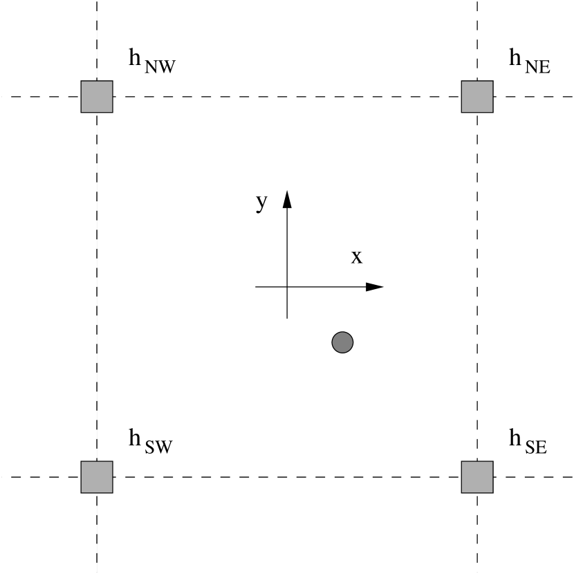
Figure 1.— The unit cell of the Fried geometry wave front sensor. Actuators are shown as solid squares, and lenslet edges as dashed lines. The $(x,y)$ coordinate system is in wave front sensor pixels. The centroid of the image produced by the lenslet is shown as the dark circle. The subaperture, when projected back on to the primary, is a square of side $a$.

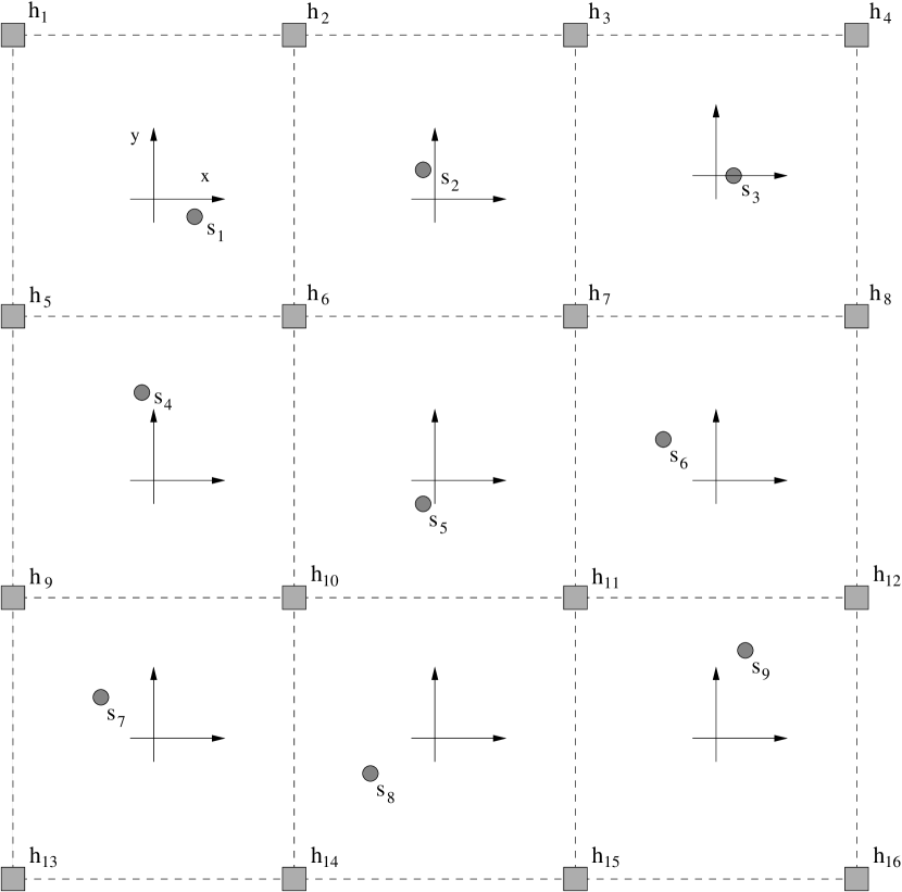
Figure 2.— A square aperture Fried geometry wave front sensor array, with sixteen actuators (shown as squares, each at a height $h_{i}$) and nine wave front sensors. Wave front slopes $s_{i}=(s_{xi},s_{yi})$ denote the instantaneous centroids of a lenslet spot in the Shack-Hartmann subaperture (in on-chip pixels).

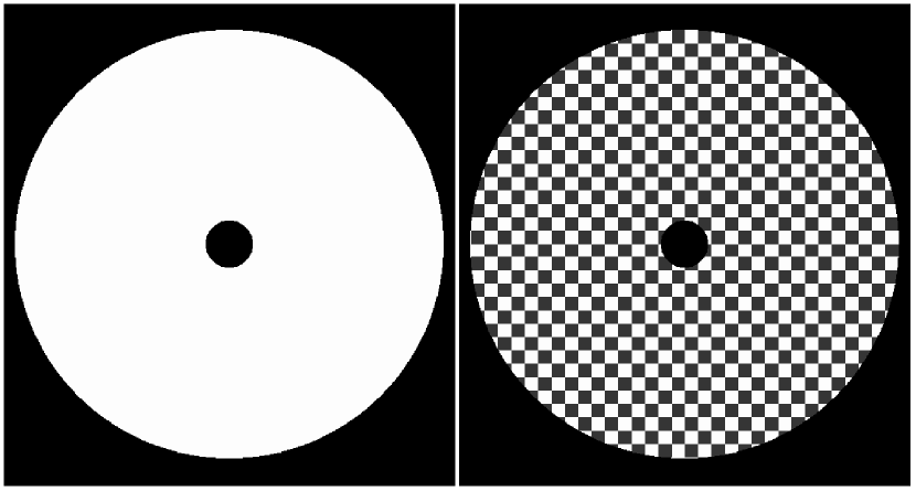
Figure 3.— The AEOS pupil and subapertures over which we calculate our simulations. Left: the telescope input pupil. The diameter of the telescope is 512 pixels, with the secondary mirror obstruction subtending 56 pixels. Right: the distribution of subapertures over the telescope pupil over which we calculate the mean $\phi_{w}$ in the incoming phase screen.

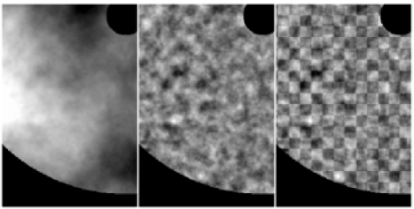
Figure 4.— Simulated Kolmogorov-spectrum and AO-corrected phase screens over the telescope pupil. Left: the incoming phase screen over a portion of the AEOS pupil with linear scaling. The AEOS secondary obstruction is shown at the upper-right. Center: the residual AO-corrected phase screen over the same portion of the AEOS pupil. Here, the linear scaling has been enhanced relative to the figure at left to show the residual structure. Right: the same residual AO-corrected phase screen as at center with waffle mode introduced, shown at the same linear scaling as at center. Here, $\phi_{w}=0.03$ radians with ${\cal W}=10$.

Figure 5.— Measured mean atmospheric $\phi_{w}$ values from 100 Kolmogorov-spectrum phase screens with the AEOS telescope and wavefront sensor subaperture geometries (top), with the mean measured value and standard deviation of the mean (bottom).

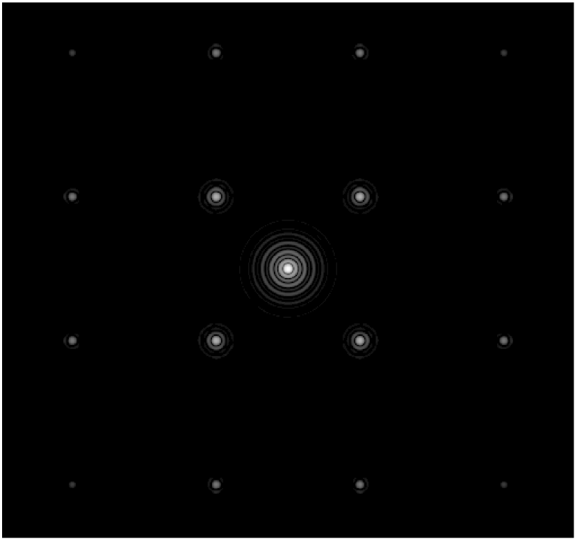
Figure 6.— Simulated monochromatic image assuming the AEOS telescope and WFS geometries with fundamental waffle mode error defined by $\phi_{w}=0.01$ radians and ${\cal W}=50$. Atmospheric correction is assumed to be perfect (i.e., no residual atmospheric phase error other than waffle). This image is on a min-max scaling with a logarithmic stretch. In this extreme case, one can clearly see the primary, secondary, and tertiary waffle spots around the central PSF (see text).

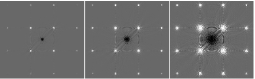
Figure 7.— Difference between simulated AEOS monochromatic PSFs with and without waffle mode error. From left to right: PSFs with waffle $\phi_{w}=0.01,~{}0.03,~{}{\rm and}~{}0.10$ can be seen in the PSFs from left to right with calculated Strehl ratios of 99.99%, 99.91%, and 99.0% respectively. In each case, atmospheric correction is assumed to be perfect (i.e., no residual atmospheric phase error other than waffle). Subtracting the perfect PSF results in a “hole” where the on-axis PSF with waffle would be, indicative of a reduced Strehl ratio in the waffle images. The antisymmetric component of the PSF due to waffle mode error is visible, though the symmetric component of the waffle mode error dominates.

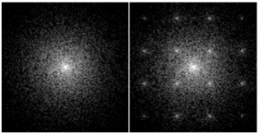
Figure 8.— Simulated AEOS monochromatic PSFs without and with waffle mode error, displayed on the same logarithmic scaling. These images assume $D/r_{0}=32$ at $\lambda=0.88~{}\micron$ with a power law AO correction with exponent 0.9 (see text). Neither read noise nor Poisson noise are included here.

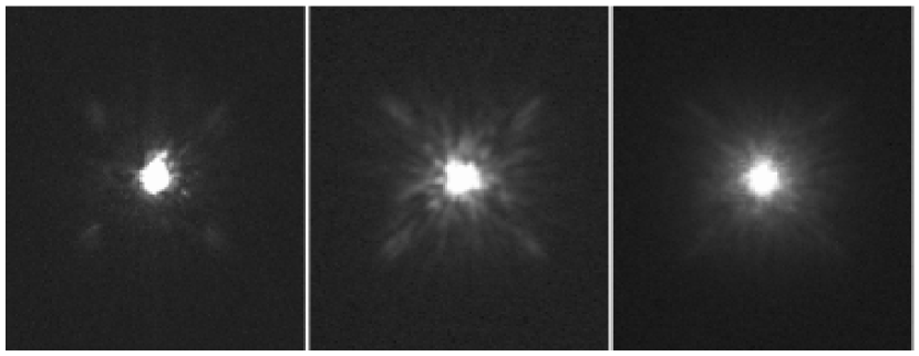
Figure 9.— At left, an AEOS Adaptive Optics $I$-band image of HR7525 acquired with the Visible Imager (VisIm) on 08 October 2002 (UT). Strehl ratio of this image has been estimated to be $\sim 20\%$. At right, a simulated AEOS Adaptive Optics $I$-band image assuming waffle mode error. The Strehl ratio of the simulated image was calculated to be $\sim 60\%$ before convolution with a Gaussian filter and and the addition of Poisson noise, which reduced the calculated Strehl to $\sim 42\%$. Other features in the observed PSF can be explained by the addition of phase errors in the input pupil.

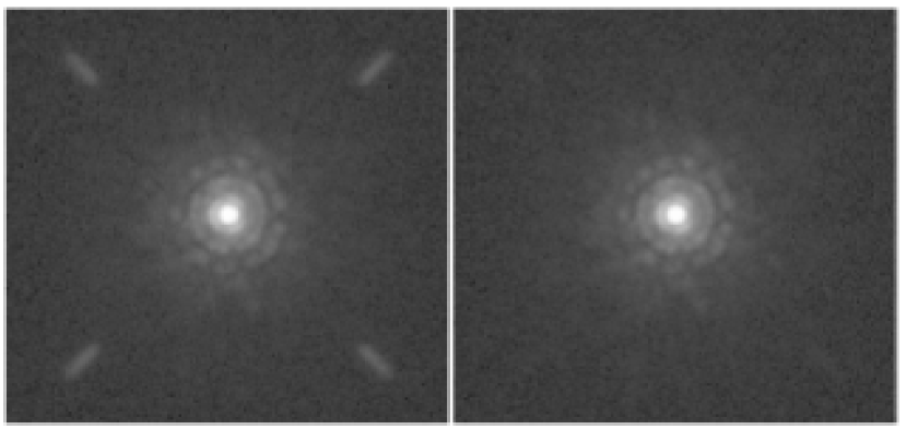
Figure 10.— Simulated AEOS $H$-band PSFs. Both of the PSFs shown here were co-added from five individual PSFs, each using a separate realization of Kolmogorov-spectrum phase screens with $r_{0}\,=\,\ 45.6{\rm\ cm}$ as input. At left is a PSF with ${\cal W}\,=\,\ 16$, with ${\cal W}\,=\,\ 4$ for the PSF at right. Poisson noise and detector read noise have been added to these PSFs. Calculated Strehl ratios are 0.79 for the PSF at left, and 0.82 for the PSF at right.

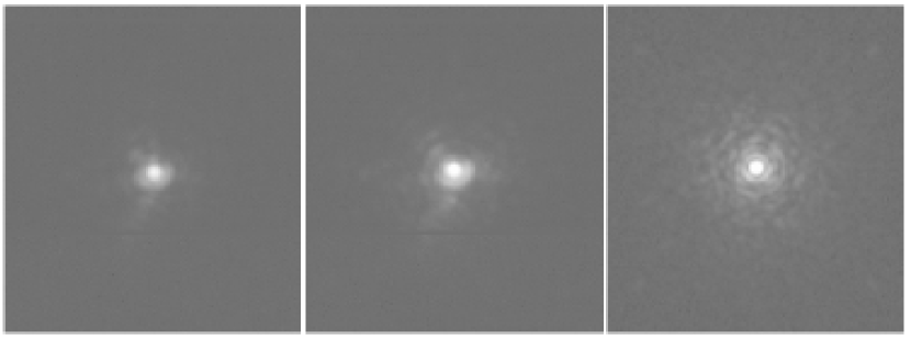
Figure 11.— Kermit Infrared Camera short-$H$-band images of the G8III star HR 4667 (HD 106714, HIP 59847) acquired on 16 April 2003 with AEOS Adaptive Optics. At left, a single 1.5 second exposure with a measured Strehl of $\sim 0.51$. A 5.0 second exposure of the same star is shown at middle. At right is a simulated PSF with a single-layer Kolmogorov-spectrum phase screen with $D/r_{0}\,=\,15.0$, with a calculated Strehl ratio of $\sim 0.55$. Since our simulations assume perfect optical surfaces, the calculated Strehl ratios for the simulated PSF are higher than those imaged with Kermit on the night of the observations.

Table 1Average Strehl Ratio for $\phi_{w}=0.01$ Radians

Waffle ($\cal W$)	$\phi_{total}$ (rad)	Strehl (%)		Waffle ($\cal W$)	$\phi_{total}$ (rad)	Strehl (%)
00.0	0.00	1.0000		20.0	0.20	0.9605
01.0	0.01	0.9999		25.0	0.25	0.9388
03.0	0.03	0.9991		30.0	0.30	0.9127
05.0	0.05	0.9975		50.0	0.50	0.7702
10.0	0.10	0.9900		75.0	0.75	0.5354
15.0	0.15	0.9776		100.0	1.00	00.2919

References

- Abreu et al. (2000) Abreu, R., Gullapalli, S. N., Rappoport, W. M., Pringle, R., & Zmek, W. P. 2000, Proc. SPIE, 3931, 300
- Bloemhof et al. (2001) Bloemhof, E. E., Dekany, R. G., Troy, M., & Oppenheimer, B. R. 2001, ApJ, 558, L71
- Bracewell (2000) Bracewell, R. N. 2000, The Fourier transform and its applications (Boston: McGraw-Hill)
- Fried (1966) Fried, D. L. 1966, Optical Society of America Journal, 56, 1372
- Fried (1977) —. 1977, Optical Society of America Journal, 67, 370
- Gavel (2003) Gavel, D. T. 2003, Proc SPIE, 4839, 972
- Glindemann & Dainty (1993) Glindemann, A., & Dainty, J. C. 1993, J. Opt. Sci. Am., 10, 1056
- Glindemann et al. (2000) Glindemann, A., Hippler, S., Berkefeld, T., & Hackenberg, W. 2000, Experimental Astronomy, 10, 5
- Goodman (1995) Goodman, J. W. 1995, Introduction to Fourier optics (New York: McGraw-Hill)
- Hardy (1998) Hardy, J. W., ed. 1998, Adaptive optics for astronomical telescopes
- Jolissant (2004) Jolissant, L. 2004, PAOLA Simulation Software (http://http://cfao.ucolick.org/software/paola.php)
- Landsman (1993) Landsman, W. B. 1993, in Astronomical Society of the Pacific Conference Series, 246–+
- Lane et al. (1992) Lane, R. G., Glindemann, A., & Dainty, J. C. 1992, Waves Random Media, 2, 209
- Makidon et al. (2003) Makidon, R. B., Sivaramakrishnan, A., Roberts, L. C., Oppenheimer, B. R., & Graham, J. R. 2003, Proc. SPIE, 4860, 315
- Oppenheimer et al. (2000) Oppenheimer, B. R., Dekany, R. G., Hayward, T. L., Brandl, B., Troy, M., & Bloemhof, E. E. 2000, Proc. SPIE, 4007, 899
- Oppenheimer et al. (2004) Oppenheimer, B. R., Digby, A. P., Newburgh, L., Brenner, D., Shara, M., Mey, J., Mandeville, C., Makidon, R. B., Sivaramakrishnan, A., Soummer, R., Graham, J. R., Kalas, P., Perrin, M. D., Roberts, Jr., L. C., Kuhn, J. R., Whitman, K., & Lloyd, J. P. 2004, Proc. SPIE, 5490, 433
- Perrin et al. (2004) Perrin, M. D., Graham, J. R., Trumpis, M., Kuhn, J., Whitman, K., Coulter, R., Lloyd, J. P., & Roberts, L. C. 2004, in 2003 AMOS Technical Conference
- Perrin et al. (2003) Perrin, M. D., Sivaramakrishnan, A., Makidon, R. B., Oppenheimer, B. R., & Graham, J. R. 2003, ApJ, 596, 702
- Porro et al. (2000) Porro, I. L., Berkefeld, T., & Leinert, C. 2000, Appl. Opt., 39, 1643
- Poyneer (2003) Poyneer, L. A. 2003, Proc. SPIE, 4839, 1023
- Poyneer & Macintosh (2004) Poyneer, L. A., & Macintosh, B. A. 2004, Journal of the Optical Society of America A, 21, 810
- Ragazzoni (1996) Ragazzoni, R. 1996, Journal of Modern Optics, 43, 289
- Roberts & Neyman (2002) Roberts, L. C., & Neyman, C. R. 2002, PASP, 114, 1260
- Roberts et al. (2004) Roberts, L. C., Perrin, M. D., Marchis, F., Sivaramakrishnan, A., Makidon, R. B., Christou, J. C., Macintosh, B. A., Poyneer, L. A., van Dam, M. A., & Troy, M. 2004, Proc. SPIE, 5490, 504
- Roddier (1988) Roddier, F. 1988, Appl. Opt., 27, 1223
- Sandler et al. (1994) Sandler, D. G., Stahl, S., Angel, J. R. P., Lloyd-Hart, M., & McCarthy, D. 1994, Optical Society of America Journal, 11, 925
- Simons & Tokunaga (2002) Simons, D. A., & Tokunaga, A. 2002, PASP, 114, 169
- Sivaramakrishnan et al. (2001) Sivaramakrishnan, A., Koresko, C. D., Makidon, R. B., Berkefeld, T., & Kuchner, M. J. 2001, ApJ, 552, 397
- Sivaramakrishnan et al. (2002) Sivaramakrishnan, A., Lloyd, J. P., Hodge, P. E., & Macintosh, B. A. 2002, ApJ, 581, L59
- Sivaramakrishnan et al. (1995) Sivaramakrishnan, A., Weymann, R. J., & Beletic, J. W. 1995, AJ, 110, 430
- Teague (1982) Teague, M. R. 1982, Optical Society of America Journal A, 72, 1199
- Troy et al. (2000) Troy, M., Dekany, R. G., Brack, G., Oppenheimer, B. R., Bloemhof, E. E., Trinh, T., Dekens, F. G., Shi, F., Hayward, T. L., & Brandl, B. 2000, Proc. SPIE, 4007, 31
- Vérinaud et al. (2005) Vérinaud, C., Le Louarn, M., Korkiakoski, V., & Carbillet, M. 2005, MNRAS, 357, L26
- Wizinowich et al. (2000a) Wizinowich, P., Acton, D. S., Shelton, C., Stomski, P., Gathright, J., Ho, K., Lupton, W., Tsubota, K., Lai, O., Max, C., Brase, J., An, J., Avicola, K., Olivier, S., Gavel, D., Macintosh, B., Ghez, A., & Larkin, J. 2000a, PASP, 112, 315
- Wizinowich et al. (2000b) Wizinowich, P. L., Acton, D. S., Lai, O., Gathright, J., Lupton, W., & Stomski, P. J. 2000b, Proc. SPIE, 4007, 2