The role of black hole mass in quasar radio activity

Abstract

We use a homogeneous sample of $\sim 300$, $0.3\lower 2.15277pt\hbox{$\;\buildrel<\over{\sim}\;$}{\rm z}\lower 2.15277pt\hbox{$\;\buildrel<\over{\sim}\;$}3$, radio-loud quasars drawn from the FIRST and 2dF QSO surveys to investigate a possible dependence of radio activity on black-hole mass. By analyzing composite spectra for the populations of radio-quiet and radio-loud QSOs – chosen to have the same redshift and luminosity distribution – we find with high statistical significance that radio-loud quasars are on average associated with black holes of masses $\sim 10^{8.6}{\rm M_{\odot}}$, about twice as large as those measured for radio-quiet quasars ($\sim 10^{8.3}{\rm M_{\odot}}$).

We also find a clear dependence of black hole mass on optical luminosity of the form ${\rm log\left(\frac{M_{BH}}{M_{\odot}}\right)_{RL}}=8.57(\pm 0.06)-0.27(\pm 0.06)({\rm M_{B}}+24.5)$ and ${\rm log\left(\frac{M_{BH}}{M_{\odot}}\right)_{RQ}}=8.43(\pm 0.05)-0.32(\pm 0.06)({\rm M_{B}}+24.5)$, respectively for the case of radio-loud and radio-quiet quasars. It is intriguing to note that these two trends run roughly parallel to each other, implying that radio-loud quasars are associated to black holes more massive than those producing the radio-quiet case at all sampled luminosities. On the other hand, in the case of radio-loud quasars, we find evidence for only a weak (if any) dependence of the black hole mass on radio power. The above findings seem to support the belief that there exists – at a given optical luminosity – a threshold black hole mass associated with the onset of significant radio activity such as that of radio-loud QSOs; however, once the activity is triggered, there appears to be very little connection between black hole mass and level of radio output.

1 Introduction

Despite the recent progress made in understanding the cosmological evolution of quasars and their host galaxies (e.g. Silk & Rees 1998; Cavaliere & Vittorini 2002; Dunlop et al. 2003; Granato et al. 2004; McLure & Dunlop 2004; Di Matteo, Springel, Hernquist 2005) there is still little known about the processes that produce the sub-class of radio-loud (RL) AGN which exhibit radio activity from powerful relativistic jets.

Neither host galaxy morphology nor large-scale environment seem to be a major determinant of a quasar’s radio activity as the two populations (or at least their brighter counterparts) are found in the same kind of bulge-dominated spheroidal galaxies (e.g. McLure et al. 1999; Schade, Boyle & Letawsky 2000; Dunlop et al. 2003) and tend to inhabit groups and clusters of similar richness (e.g. McLure & Dunlop 2001; Wold et al. 2001). At face value, these findings imply that enhanced jet activity from AGNs is associated with the pc/sub-pc scale behavior of a galaxy, and more specifically related to some properties of its central black hole. The extraction and collimation of energy from the accretion disk to form jets most likely involves some magnetohydrodynamic mechanism (Blandford & Payne 1982) and/or the spin of the black-hole (Blanford & Znajeck 1977; Blandford 2002). In addition, the mass of the central black hole could play an important role in regulating the radio-loud/radio-quiet dichotomy.

The issue of a possible dependence of radio activity on black hole mass has recently been the subject of many scientific debates. A number of authors (e.g. Laor et al. 2000; McLure & Dunlop 2002; Dunlop et al. 2003; Marziani et al. 2003; McLure & Jarvis 2004) have concluded that radio-loud sources (both quasars and radio-galaxies) are systematically associated with black holes of greater mass than their radio-quiet (RQ) counterparts. The proposal, first made by Laor (2000), that there exists a threshold black hole mass below which a quasar cannot be radio-loud was further confirmed by the clustering results of Magliocchetti et al. (2004) who find local (${\rm z\lower 2.15277pt\hbox{$\;\buildrel<\over{\sim}\;$}0.3}$) radio galaxies to be powered by black holes with masses ${\rm M_{BH}\lower 2.15277pt\hbox{$\;\buildrel>\over{\sim}\;$}10^{9}M_{\odot}}$, about an order of magnitude higher than those found for radio-quiet quasars by means of the same statistical analysis (see e.g. Porciani, Magliocchetti & Norberg 2004). Furthermore, some author also claim that there is a continuous relationship (although with a large scatter) between radio-power and black hole mass that holds over about a decade in radio power, from local ’inactive’ galaxies (Franceschini, Vercellone & Fabian 1998), to powerful radio-galaxies (McLure et al. 2004) and quasars (e.g. Lacy et al. 2001; McLure & Jarvis 2004).

On the other side, other authors have argued strongly against any dependence of radio luminosity on black hole mass and the existence of a threshold mass above which the fraction of radio-loud vs radio-quiet sources drastically increases; in fact, they find evidence for radio-loud objects associated with black holes with masses as low as ${\rm 10^{6}M_{\odot}}$ (e.g. Oshlack et al. 2002; Ho 2002; Woo & Urry 2002a,b; Snellen et al. 2003. See however the dissenting view of Jarvis & McLure 2002 who re-analysed the Oshlack et al. 2002 sample by taking into account corrections due to Doppler boosting effects and the geometry of the broad-line region).

The aim of this work is to reexamine the issue of radio activity vs. black hole mass by investigating the spectral properties of a new, homogeneous sample of $\sim 300$ radio-loud quasars – spanning the redshift range $0.3\lower 2.15277pt\hbox{$\;\buildrel<\over{\sim}\;$}{\rm z}\lower 2.15277pt\hbox{$\;\buildrel<\over{\sim}\;$}3$ – obtained by the joint use of the FIRST and 2dF Quasar Redshift Surveys. Average virial mass estimates are derived for these objects and compared to those of a similar-size sample of radio-quiet quasars, also drawn from the 2dF QSO survey. The two samples are selected to have the same redshift and magnitude distributions to avoid any biases due to cosmological evolution and/or selection. We also present estimates of black hole mass as a function of optical and radio luminosities for these sources. Throughout this paper we will assume $\Omega_{0}=0.3$, $\Lambda=0.7$, $\rm h_{0}=0.7$ as the latest results from the joint analysis of CMB and 2dF data indicate (see e.g. Lahav et al. 2002).

2 Data

For our analysis we make use of the catalogue of radio-loud quasars presented in Cirasuolo et al. (2003a) and Cirasuolo, Magliocchetti & Celotti (2005). Briefly, a catalogue of 352 sources has been obtained by matching together objects from the FIRST (Faint Images of the Radio Sky at Twenty centimeters) survey (Becker et al. 1995) and the 2dF QSO redshift survey (Croom et al. 2004).

The FIRST survey includes 811,117 sources (April 2003 release used for this work) observed at 1.4 GHz down to a flux limit S${}_{\rm 1.4GHz}\simeq$0.8 mJy and is substantially complete. Its completeness has been estimated to be 95 per cent at 2 mJy and 80 per cent at 1 mJy. The survey covers a total of about 9033 square degrees on the sky (8422 square degrees in the North Galactic cap and 611 in the South Galactic cap). Point sources at the detection limit of the catalogue have positions accurate to better than 1 arcsec (90 per cent confidence level).

The 2dF QSO redshift survey (2QZ) includes $\sim$21,000, $18.25\leq{\rm b_{J}}\leq 20.85$, quasars with reliable spectra and redshift determinations covering two $75^{\circ}\times 5^{\circ}$ declination strips centered on $\delta=-30^{\circ}$ (South Galactic cap) and $\delta=0^{\circ}$ (North Galactic cap). In order to guarantee a large photometric completeness ($>90$ per cent) for quasars within the redshift $0.3\leq{\rm z}\leq 2.2$, the following color selection criteria were applied: $(u-b_{j})\leq 0.36$; $(u-b_{j})<0.12-0.8\;(b_{j}-r)$; $(b_{j}-r)<0.05$. Spectroscopic observations of the input catalogue were made with the 2-degree Field (2dF) instrument at the Anglo-Australian Telescope. The spectra were classified both via cross-correlation with specific templates (AUTOZ, Croom et al. 2004) and by visual inspection.

The FIRST and 2QZ surveys overlap in the region $9^{h}\;50^{m}\leq{\rm RA(2000)}\leq 14^{h}\;50^{m}$ and $-2.8^{\circ}\leq{\rm Dec(2000)}\leq 2.2^{\circ}$. In this region there are 10,110 optical quasars from the 2QZ and $\sim$45,500 radio sources down to S_1.4GHz=1 mJy from the FIRST catalogues. Not all these radio sources correspond to separate objects. As described in Cirasuolo et al. (2003a), the authors used the algorithm developed by Magliocchetti et al. (1998) to collapse multi-component sources into single objects having radio fluxes equal to the sum of the components. All the optical-radio pairs with offsets of less than 2 arcsec are considered true optical identifications. The value of 2 arcsec was chosen, after a careful analysis, as the best compromise between maximizing the number of real associations (estimated to be $\sim 97$ per cent) and minimizing the contribution from spurious identifications (a negligible 5%) (Magliocchetti & Maddox 2002). In addition, in order to verify the reliability of the associations, all the radio-optical pairs obtained from the collapsing algorithm were checked by eye on the FIRST image cutouts.

This procedure has lead to a homogeneous sample 352 quasars (113 presented in Cirasuolo et al. 2003a, while the remaining 239 given in Cirasuolo et al. 2005) with good redshift determinations from the 2QZ and with radio fluxes ${\rm S_{1.4GHz}\geq 1}$ mJy over an effective area of 284 square degrees. Due to the 2QZ and FIRST flux limits all these sources can be considered radio-loud whether one uses the criterion of a radio-to-optical ratio $R^{\*}_{\rm 8.5GHz}\lower 2.15277pt\hbox{$\;\buildrel>\over{\sim}\;$}10$ (corresponding to $R^{\*}_{\rm 1.4GHz}\lower 2.15277pt\hbox{$\;\buildrel>\over{\sim}\;$}30-40$ for objects with a spectral index $\alpha_{\rm R}=0.8$; Kellermann et al. 1989) or a threshold of $\rm log_{10}P_{5GHz}\sim 24$ [W Hz^-1sr^-1] as used by Miller et al. (1990).

The above radio-quasar sample corresponds to about 3.5 per cent of the original 2dF quasar population. This value is somewhat lower than what found in previous works ($\sim$ 10-20 per cent; White et al. 2000; Hewett, Folz & Chaffee 2001; Ivezic et al. 2002). As demonstrated by Cirasuolo et al. (2003a; 2003b), the reason for this finding originates from the fact that the radio-loud fraction is a function of absolute optical luminosity so that the low radio-loud fraction of the 2QZ/FIRST sample is due to the relative optical faintness of the 2QZ quasars.

Luminosities for the above sample were obtained by converting magnitudes from the the $b_{\rm J}$ to the B band. The mean $B-b_{\rm J}$ was computed from the composite quasar spectrum compiled by Brotherton et al. (2001) from $\sim 600$ radio-selected quasars in the FIRST Bright Quasar Survey (FBQS). The K-correction in the B band has also been computed from the Brotherton et al. (2001) composite quasar spectrum.

Since the aim of this work is to analyze the (optical) spectral differences between radio-loud (RL) and radio-quiet (RQ) quasars, we have generated a sample of 352 radio-quiet QSOs by extracting sources at random from the 2QZ survey in the same area covered by our radio-loud catalogue. These sources were chosen to have the same redshift and magnitude distributions as the radio-loud sample (see figures 1, 2) in order to exclude any possible bias due to cosmological and luminosity evolution and/or selection in our analysis. The application of the one-dimensional Kolmogorov-Smirnov (KS) test finds that both the optical luminosity and the redshift distributions of the RL and RQ samples are indistinguishable: the probabilities of getting larger KS statistics are p=0.99 and p=0.76 respectively. These probabilities are so high because the RQ QSOs have been picked by hand to have the same redshift distribution as the RL QSOs. This also confirmed in the case of the z-$\rm M_{B}$ distribution; application of the two-dimensional KS test gives p=0.82.

Optical spectra for both radio-loud and radio-quiet quasars were subsequently obtained from the 2dF QSO survey public release (http://www.2dfquasar.org). Sixty one of the radio-loud sources in our catalogue did not have spectra available in the archive, leaving 291 that did. It is likely that the reason for this incompleteness arises from not having included (as their spectra are not publicly available) from the 2QZ survey those sources belonging to the Brotherton et al. (1998) sample. We have therefore made sure that when the radio-loud sources without available spectra are included in the sample the redshift and luminosity distributions are still consistent with those of the radio-quite sample. The one-dimensional KS test gives p=0.82 and p=0.52 for the redshift and magnitude distributions respectively and the two-dimensional KS test gives p=0.71 – all very consistent with coming from the same distribution. Figures 1 and 2 show these distributions, where the dashed histograms indicate the total radio-loud sample, while the dotted ones show the portion of radio-loud sample with available optical spectra. Based on the above results we are confident that the two sets represent the same underlying population and in the following analysis we will use the sub-sample of 291 radio-loud quasars to compare their spectral properties with those of radio-quiet sources.

Figure 1: Redshift distribution for the samples under examination. The solid line is for radio-quiet sources, the dashed line for radio-loud sources, and the dotted line represents those radio-loud quasars with available optical spectrum from the 2dF QSO survey.

Figure 2: Luminosity distribution for the samples under examination. The line coding is as in figure 1.

3 Constructing Composite Spectra

Figure 3: Continuum normalized composite spectra for our sample of radio-quite (on top) and radio-loud (on bottom) QSOs.

Figure 4: Composite spectra for the sample of radio-quiet QSOs binned in B-band absolute magnitude. The M_B ranges for the spectra from bottom to top are: -27 to -30, -27 to -25, -25 to -24 and -21 to -24 mag. The very top curve is for all the RQ QSOs and is the same spectrum as in figure 3. From the spectral ranges it is possible to see both the redshift dependent selection effects and the cosmological luminosity evolution of QSOs.

Figure 5: Same as figure 4 only for radio-loud QSOs.

The typical 2dF spectrum has a dispersion of 4.3 Å per pixel and a resolution of $\simeq 9$ Å over the range 3700-7900 Å. The median signal-to-noise ratio is $\sim$5 pixel^-1 (Croom et al. 2002). This noise level is too large to accurately measure individual line widths. Instead we must rely on composite spectra to reveal spectral properties of the population as a whole with higher signal to noise.

The composite spectra are constructed by performing the following steps on each of the contributing spectra. First, cosmic rays and bad pixels are removed. Then, since 2dF spectra are not flux-calibrated, we normalized each spectrum to a local continuum level. The continuum spectrum is calculated by removing the regions in the spectrum that contain known emission features and then interpolating the spectrum over these regions. The interpolation was done by taking the median of the spectrum in two portions of spectra on either side of each line region and then linearly interpolating between them. The wavelength ranges used for the spectral features and the adjacent interpolation regions are the same as in Croom et al. (2002). We did a further 50 pixel wide median smoothing which we judge to be the best compromise between minimize the noise in our continuum spectrum and at the same time preserve its large-scale features. The original spectrum was then divided by the continuum spectrum. This continuum-normalized spectrum is then shifted to the rest frame-wavelength according to the redshift measured by the 2dF survey and then it is linearly interpolated at intervals of every 1 Å. The final composite spectrum is made by taking the median of these individual QSO spectra at each 1 Å interval or “pixel”.

The composite spectra for all the radio-loud and radio-quiet QSOs are shown in figure 3. As a result of the spectral range of the 2dF spectrograph, no single QSO contributes to the full wavelength range of the spectra shown here. It can be seen that the noise level varies over the length of the spectra, becoming largest at either end, because the number of contributing spectra changing with wavelength.

The QSO samples are further divided into four $\rm M_{B}$ bins and the composite spectra are calculated and shown in figures 4 and 5. The numbers of quasars contributing to each composite spectrum at the different magnitudes are: 73 RL and 92 RQ quasars in the $-21\leq\rm M_{B}<-24$ range; 96 RL and 122 RQ in the $-24\leq\rm M_{B}<-25$ range; 112 RL and 129 RQ in the $-25\leq\rm M_{B}<-27$ range and 6 RL and 4 RQ in the $-27\leq\rm M_{B}<-30$ range. Note that the luminosity interval for which a single line can be measured is limited. Any further division of the samples in $\rm M_{B}$ tends to increase the noise to such a level that comparisons of the RL and RQ composite spectra are not very meaningful.

One might be concerned that coarsely binning the sample in luminosity might obscure the meaning of any differences between the RL and RQ composite spectra – the differences could be caused by QSOs of the same luminosity or different luminosities. However, it can easily be shown that if the RL and RQ samples have the same luminosity distribution then any difference in their composite spectra must be caused by differences in QSOs of the same luminosity (see appendix). As shown in section 2, our samples are consistent with having the same luminosity distribution. In addition, the bootstrap method for estimating errors on the line widths, discussed in the next section, should take into account any coincidental differences in the luminosity distributions. For these reasons it makes sense to use composite spectra in coarse luminosity bins to compare the black hole masses of the RL and RQ quasars.

In addition, it has been shown that more generally radio emission does not exhibit any tight correlation with visible luminosity (e.g. Cirasuolo et al. 2003b), since sources with a particular optical luminosity can have radio powers spanning up to three orders of magnitude. This implies that our sample is representative in this respect.

It is probable that there are other “hidden” properties that are correlated with both radio emission and particular spectral properties, either because of a common cause or a direct causal connection. There have been claims that various spectral properties of QSOs depend on their position on the so-called Eigenvector 1 (E1) parameter space, which relates the full width at half maximum (FWHM) of the broad component of H${\beta}$ (H${\beta}_{\rm BC}$) with the ratio between the equivalent width of H${\beta}_{\rm BC}$ and that of the Fe_II complex centered at $\lambda 4570$ (see e.g. Marziani et al. 2003; Sulentic et al. 2004 and references therein). Unfortunately, due to the limitations of the 2dF spectra we cannot accurately measure the Fe_II complex and test for the above effect. However, our composite spectrum for radio-loud sources does appear remarkably similar to those of the Marziani et al. B1 population (Marziani, private communication), giving us some confidence that the majority of our radio-loud quasars falls in this category and therefore constitutes a roughly homogeneous sample also in the E1 space.

4 Fitting Line Widths

Figure 6: Blowup of the spectra shown in figure 3 around the Mg II line. The thick upper curves are the composite spectra for RQ sources with and without the contaminating lines subtracted, in this case Fe II . The thick curves on the bottom are the same spectra for the RL quasars. The thin spectrum at the top is the RL spectrum reproduced and shifted up for better comparison with the RQ spectrum.

Figure 7: Blowup of the spectra shown in figure 3 around the C III] line. The identities of the spectra are the same as in figure 6. There is also a Si III] line at 1892Å  that was not subtracted. Note that the removal of the Al III lines does not significantly change the FWHM of the C III] + Si III] lines, which are found to be very similar in the two RL and RQ cases (see Table 1).

Figure 8: Blowup of the spectra shown in figure 3 around the C IV line. The identities of the spectra are the same as in figure 6. The blueshift of these lines relative to Mg II is evident when one compares the positions of these emission lines in the restframe (as marked by the dashed lines). There is no significant difference in the width of the RL and RQ C IV lines (see Table 1).

The widths of the Mg II , C III] and C IV lines are measured from the composite spectra in figure 3 and the luminosity-binned spectra in figures 4 and 5. The widths of the H$\beta$ and Ly$\alpha$ lines are not used here because we find the noise in these two regions of the composite spectra to be too large to make useful measurements. The regions around the Mg II , C III] and C IV lines are shown in more detail in figures 6, 7 and 8.

Contaminating lines are removed before the widths of the three major lines are measured. In each case, the main line and the contaminating lines are fit to a model and then the model for the contaminating lines alone is subtracted from the spectrum. Each contaminating line is modeled as a Gaussian and the main lines – Mg II , C III] and C IV – are modeled as two Gaussians, one with a broad and one with a narrow component. The relative centers of the lines are fixed, but the redshift is allowed to vary during the fit.

Note that there is a Fe II feature longword of the Mg II line (see figures 3 and 6). This feature is subtracted, but does not have any significant effect on the measured line width because Fe II is well out in the wing of the Mg II line. An Al II doublet is subtracted from the C III] line (see figure 7). Si V and He II are removed from the C IV line (figure 8). None of these lines have a significant effect on the measured FWHM line widths.

We tested several methods for measuring the line widths and found them all to be consistent. One was to use the FWHM of the model that was fit to the data in order to remove the contaminating lines. This method assumes that the line shape is similar to the double Gaussian used to model it. Another method was to median smooth the spectrum over 5 pixels and then find the FWHM. The widths reported in this paper were calculated by first finding the maximum pixel value within the line. To reduce the dependence on noise in a single pixel, we take the median of the maximum pixel value and its four nearest neighbors. Using this as the peak value of the line we find the closest pixel on each side of the line with a value below half the peak value. It was found that this last method has the least variance and makes a minimum of assumptions about the shape of the line while agreeing very well with the other two methods. We also calculated an inter-percentile velocity (IPV) width by integrating the spectra around the peak of the line and finding the region symmetrically surrounding the peak that contains 76% of the total (corresponding to the area within the FHWM of the Gaussian). We found that in comparison to the FWHM the IPV was more sensitive to the wings of the line and more strongly dependent on the subtraction of the contaminating lines. We therefore discarded it in favor of the FWHM. Table 1 shows the FWHM measures of the line widths for the radio-loud and radio-quite populations. The values derived for our sample of radio-quiet quasars are in very good agreement with those obtained by Corbett et al. (2003). Note that the entire broad line width is used; no attempt is made to separate narrow and broad components.

Errors in the line widths are derived by the bootstrap method. Spectra are drawn at random from the samples of continuum-normalized spectra with replacement – 352 for the radio-quite population and 291 for the radio-loud one. From these a composite spectrum is constructed in the same way as discussed in § 3 and the line widths are measured as discussed above. This process is repeated 1000 times. The errors given in table 1 are the 68 percentile (corresponding to 1-sigma) confidence regions derived from the resulting distributions.

Table 1: Widths of the Mg II , C III] and C IV broad lines. These are all consistent for radio-loud and radio-quiet sources except in the case of Mg II .

	Mg II	C III]	C IV
Radio-loud (FWHM)	$4710^{+210}_{-220}\mbox{ km s${}^{-1}$}$	$5810^{+310}_{-320}\mbox{ km s${}^{-1}$}$	$5410^{+520}_{-440}\mbox{ km s${}^{-1}$}$
Radio-quiet (FWHM)	$3960^{+250}_{-290}\mbox{ km s${}^{-1}$}$	$5970^{+270}_{-200}\mbox{ km s${}^{-1}$}$	$5020^{+390}_{-390}\mbox{ km s${}^{-1}$}$

5 Results

Table 1 shows that of the three lines analyzed in our work only the Mg II line has a width that is measurably correlated with radio activity while the C III] and C IV line widths are consistent with being the same in the RL and RQ samples. This is perhaps not too surprising given that Mg II is a low-ionization line that is believed to originate in virialized gas clouds, which in turn implies that, like for H$\beta$, its line width can be considered as a good tracer of the quasar’s black hole mass (McLure & Jarvis 2002). The same cannot be said of C IV since there is strong evidence for a systematic blueshift of this line indicating that it is more likely to be associated with some form of outflow rather than produced by virialized clouds (e.g. Marziani et al. 1996; Bachev et al. 2004).

The blueshift of the C IV lines can be clearly seen in figure 8. The relative blueshift between the peaks of the Mg II and C IV lines was measured in the composite spectra and the bootstrap realizations. The relative shifts were found to be $-400^{+300}_{-400}\mbox{ km s${}^{-1}$}$ for the RL sample and $-600^{+200}_{-200}\mbox{ km s${}^{-1}$}$ for the RQ sample. A larger C IV blueshift in the RQ quasars is in agreement with previous findings (e.g. Marziani et al. 1996, Richards et al. 2002 and Bachev et al. 2004).

In contrast to C IV , the C III] lines in the RL and RQ composite spectra are remarkably similar although in this case the Si III] line – that we did not attempt to subtract (figure 7) – makes the interpretation difficult. It does seem as though the only differences between the RL and RQ line profiles in the case of C III] are attributable to differences in the Si III] lines.

We use the McLure & Jarvis (2002) estimator to derive the average black hole mass for the different samples of radio-loud and radio-quiet quasars. Under the assumption that the motion of the Mg II -emitting material is virialized, one can estimate the central black hole mass via the expression:

$${\rm M_{BH}}=G^{-1}{\rm R_{[Mg\,{\scriptsize II}~{}]}}{\rm V_{[Mg\,{\scriptsize II}~{}]}}^{2},$$ (1)

where $\rm R_{[Mg\,{\scriptsize II}~{}]}$ is the radius of the broad-line region and $\rm V_{[Mg\,{\scriptsize II}~{}]}$ is the Keplerian velocity of its gas, which can be written as $f\cdot{\rm FWHM_{[Mg\,{\scriptsize II}~{}]}}$. The geometric factor $f$ relates the FWHM to the intrinsic Kaplerian velocity of the emitting gas in the Mg II region. Assuming random isotropic orbits, $f=\sqrt{3}/2$ (see McLure & Jarvis 2002 and McLure & Dunlop 2004 for further considerations on this issue). To relate the radius of the Mg II region to the luminosity at 3000Å  we use the steeper relation derived by McLure & Dunlop (2004) for high-luminosity (SDSS) quasars, such as those considered in this analysis, instead of the fit given in McLure & Jarvis (2002). We therefore adopt:

$$\rm R_{[Mg\,{\scriptsize II}~{}]}=(18.5\pm 6.6)\;[\lambda L_{3000}/10^{37}{\rm W}]^{(0.62\pm 0.14)}.$$ (2)

With the above relations, the black-hole mass estimator can then be written as:

$$\frac{\rm M_{BH}}{M_{\odot}}=f\cdot 3.2\;\left(\frac{\lambda{\rm L_{3000}}}{10^{37}{\rm W}}\right)^{0.62}\left(\frac{\rm{FWHM_{\rm Mg\,{\scriptsize II}~{}}}}{\rm{kms^{-1}}}\right)^{2},$$ (3)

with ${\rm L_{bol}}=5.9\cdot\lambda{\rm L_{3000}}$, and

$${\rm M_{B}}=-2.66(\pm 0.05)\;{\rm log[L_{bol}/W]}+79.36(\pm 1.98),$$ (4)

where ${\rm L_{bol}}$ is the bolometric luminosity and ${\rm M_{B}}$ is the absolute B magnitude (see McLure & Dunlop 2004 for further details).

Our mass estimates are derived from equations (2) through (4) using the median values of the B magnitudes for the radio-loud and radio-quiet samples in equation (4). Note that these median values have not been calculated for the entire sample but only for those sources that contribute to the composite Mg II line, i.e. 237 radio-loud and 220 radio-quiet quasars. The average black hole masses for the two populations of radio-loud and radio-quiet quasars then read:

$${\rm log\left(\frac{M_{BH}}{M_{\odot}}\right)_{RL}}=8.56\pm 0.04$$ (5)

$${\rm log\left(\frac{M_{BH}}{M_{\odot}}\right)_{RQ}}=8.30\pm 0.06,$$

which shows with a confidence level $\lower 2.15277pt\hbox{$\;\buildrel>\over{\sim}\;$}3\sigma$ that black holes associated with radio-loud quasars are in general about twice as massive as those producing the radio-quiet case.

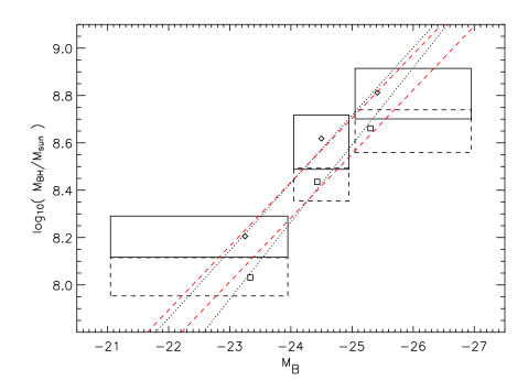
Figure 9: The black hole mass derived from Mg II line widths in different B-band absolute magnitude bins. The boxes show the range of the $\rm M_{B}$ bins and the one sigma error bars in $\log_{10}\rm M_{\rm BH}$. The solid boxes are for the radio-loud sample and the dashed boxes are for radio-quite sample. The median values are shown by squares and diamonds. The dotted lines are the best fits to the data, while the dashed lines show the fits when only normalization is allowed to vary (see section 5).

Figure 10: The black hole mass as derived from Mg II line widths in different bins of radio power. As in figure 9, the boxes show the range of the $\rm{\log_{10}\;P\;[W/Hz/sr]}$ bins and the one sigma error bars in $\log_{10}\rm M_{\rm BH}$. The dotted line is the best fit to the data (see section 5).

To further investigate this difference we examine the line widths and black hole masses for the QSO samples binned in absolute B-band magnitudes (figures 4 and 5). Figure 9 shows the black holes masses in these bins. Linear fits to the data give

$${\rm log\left(\frac{M_{BH}}{M_{\odot}}\right)_{RL}}=8.57(\pm 0.06)-0.27(\pm 0.06)({\rm M_{B}}+24.5)$$ (6)

$${\rm log\left(\frac{M_{BH}}{M_{\odot}}\right)_{RQ}}=8.43(\pm 0.05)-0.32(\pm 0.06)({\rm M_{B}}+24.5)$$ (7)

The RL and RQ normalizations are inconsistent with each other at the two sigma level and agree with the values derived from using the whole luminosity range (5). On the other hand, the slopes are consistent with being equal and indicate that the two populations follow a very similar relationship where the black hole mass is almost linearly dependent on luminosity, $\rm{M_{BH}}\propto{\rm{L_{B}}^{0.7}}$ (see equation 4).

Corbett, et al.(2003), using a much larger sample from 2dF QSO survey, found a relation between the Mg II line width and B-band luminosity that is given by $\log(v)=1.43(\pm 0.4)+0.048(\pm 0.009)\log(L_{b})$ (no distinction was made between RL and RQ QSOs). This translates into a slope of $0.27$ in the relations above, value which is within 1-sigma of both of our RL and the RQ slopes. We can therefore justifiably assume that the slope is the same for RL and RQ QSOs and fit for just the normalization, or typical black hole mass. These fits read

$${\rm log\left(\frac{M_{BH}}{M_{\odot}}\right)_{RL}}=8.57(\pm 0.06)-0.27(\rm M_{B}+24.5)$$ (8)

$${\rm log\left(\frac{M_{BH}}{M_{\odot}}\right)_{RQ}}=8.42(\pm 0.04)-0.27(\rm M_{B}+24.5),$$ (9)

and indicate – together with equations (6) and (7) – that at all luminosities RL QSOs show a systematic trend to be more massive than RQ ones. More specifically one has that for a given luminosity, a typical radio-loud QSO has a black hole mass that is about $1.4$ times as massive as a radio-quite QSO of the same B-band luminosity. Note that this result could also be interpreted as evidence for the hypothesis that, at each given luminosity, there is a critical black hole mass that is required to produce relevant radio activity.

The above results are in good agreement with the findings of McLure & Jarvis (2004) who analysed two samples of radio-loud and radio-quiet quasars drawn from the SDSS Quasar Catalog II (Schneider et al. 2003) so to be indistinguishable in terms of redshift and optical luminosity distributions. The above authors in fact conclude that the average black hole mass associated to radio-loud quasars is about twice that of radio-quiet quasars. They also report that such black hole mass difference is constant over the full luminosity range covered by their samples. Jarvis & McLure (2004) find black hole masses that are slightly greater than those derived in this work, but the difference is most likely to be attributed to the different selection criteria of the 2dF and SDSS surveys, the latter one preferentially selecting brighter quasars than 2QZ.

Another interesting result that can be obtained from our samples is the relationship between black hole mass and radio luminosity. The trend is illustrated in figure 10 for the population of radio-loud quasars. A linear fit to the data leads to

$${\rm log\left(\frac{M_{BH}}{M_{\odot}}\right)_{RL}}=8.60(\pm 0.06)+0.15(\pm 0.08)({\rm\log_{10}P}-25)$$ (10)

(where the radio power is measured at 1.4 GHz and given in [W/Hz/sr] units), which shows that radio luminosity and black hole mass are very loosely correlated since the dependence – if any – between these two quantities is much weaker than in the black hole/optical luminosity case.
The above results can be interpreted as evidence for the fact that while optical/nuclear emission is directly related to the mass of the black hole that produces the quasar signal, radio luminosity is not. Black hole mass in RL quasars merely plays a marginal “threshold” role whereby, for a given optical luminosity, only the more massive quasars will develop significant radio activity. However, once the activity is triggered, there is no significant evidence for a connection between black hole mass and the level of radio output (see also Magliocchetti et al. 2004).

6 Conclusions

We have made use of a homogeneous sample of $\sim 300$, $0.3\lower 2.15277pt\hbox{$\;\buildrel<\over{\sim}\;$}{\rm z}\lower 2.15277pt\hbox{$\;\buildrel<\over{\sim}\;$}3$, radio-loud quasars drawn from the FIRST and 2dF QSO surveys to estimate possible dependences of radio activity on black-hole mass. By analyzing composite spectra for the populations of radio-quiet and radio-loud QSOs – chosen to have the same redshift and luminosity distribution – we find with high statistical significance that radio-loud quasars are on average associated to black holes of masses $\sim 10^{8.56\pm 0.04}{\rm M_{\odot}}$, about twice as large as those obtained for radio-quiet quasars ($\sim 10^{8.30\pm 0.06}{\rm M_{\odot}}$).

The above result is also verified when one splits the two samples in luminosity bins. In fact, we observe a clear dependence of black hole mass on optical luminosity of the form ${\rm log\left(\frac{M_{BH}}{M_{\odot}}\right)_{RL}}=8.57(\pm 0.06)-0.27(\pm 0.06)({\rm M_{B}}+24.5)$ and ${\rm log\left(\frac{M_{BH}}{M_{\odot}}\right)_{RQ}}=8.43(\pm 0.05)-0.32(\pm 0.06)({\rm M_{B}}+24.5)$, respectively for the case of radio-loud and radio-quiet quasars. These trends run parallel to each other, implying that radio-loud quasars are associated to black holes about $1.4$ times more massive than those producing the radio-quiet case at all sampled luminosities. On the other hand, in the case of radio-loud quasars, we only find evidence for a marginal (if any) dependence of the black hole mass on radio power (${\rm log\left(\frac{M_{BH}}{M_{\odot}}\right)_{RL}}=8.60(\pm 0.06)+0.15(\pm 0.08)({\rm\log_{10}P}-25)$).

Our results allow a number of important conclusions to be drawn:
i) There exists a strong correlation between level of optical/nuclear emission and mass of the black hole producing the quasar. The same correlation holds for both radio-loud and radio-quiet quasars, but with different zero-points.
ii) Radio-loud quasars are on average more massive than radio quiet ones at all (optical) luminosities.
iii) Black hole mass plays a partial, threshold, role in determining the radio activity that gives rise to the population of radio-loud quasars. Our findings are further support for the existence – at each given optical luminosity – of a threshold black hole mass associated with the onset of significant radio activity such as that of radio-loud QSOs; however, once the activity is triggered, there appears to be very little evidence for a connection between black hole mass and level of radio output (see also Magliocchetti et al. 2004).

An important issue to stress is that, while the absolute values associated to the various quantities analyzed in this paper might be somehow affected by calibration effects (see e.g. section 5), all the results that compare the two populations of radio-loud and radio-quiet quasars are not, as any difference in the zero-point calibrations would cancel out during the comparison process. Even though the analyzed samples are too small to investigate for any presence of a different cosmological evolution of the two RQ and RL populations, the above statement, together with our choice of selecting two samples that were as“indistinguishable” as possible (in number of sources, luminosity and redshift distributions), give us confidence in the reliability of the results.

As a final remark we note that, since we have chosen two samples matched in optical luminosity, the fact that RL quasars harbor on average more massive black holes implies that these sources accrete at a lower fraction of their Eddington limit than their RQ counterparts. Whether this result can be seen as evidence that radio-loud and radio-quiet quasars are two distinct populations or whether this can simply be interpreted by saying that radio-loud quasars mark a different (possibly later) stage of evolution of radio-quiet quasars is still unclear and we plan to tackle this issue in a forthcoming paper.

Appendix A interpretation of composite spectra

If the luminosity distribution of the radio-loud and radio-quite QSOs are the same then the difference in their composite spectra must reflect a difference in the spectra of radio-loud and radio-quite QSOs of the same luminosity. This is important because a difference in line width can then be directly interpreted as a difference in black hole mass. If this were not the case, we might be comparing radio-loud QSOs at one luminosity to radio-quite QSOs at another luminosity and then the derived difference in black hole mass might just be the result of this difference in luminosity. In that case we would not be able to conclude that radio-loud and radio-quite of the same visible luminosity tend to have black holes of different masses.

Let the QSO spectra be binned into arbitrarily narrow bins in visible luminosity $L$. Let us say there are a total of $N$ QSOs in the sample and there are $n(L)$ QSOs in the luminosity bin centered on $L$. The composite spectrum $f_{c}(\lambda)$ is the average of these spectra at fixed wavelength. The average difference between the composite spectra of the radio-loud and radio-quite is

$$\left\langle f_{c}^{\rm RL}(\lambda)-f_{c}^{\rm RQ}(\lambda)\right\rangle\;\;\;\;\;\;\;\;\;\;\;\;\;\;\;\;\;\;\;\;\;\;\;\;\;\;\;\;\;\;\;\;\;\;\;\;\;\;\;\;\;\;\;\;\;\;\;\;\;\;\;\;\;\;\;\;$$

$$=\frac{1}{N_{\rm RL}}\sum_{L}\left\langle\sum_{i}f^{\rm RL}_{i}(\lambda,L)\right\rangle-\frac{1}{N_{\rm RQ}}\sum_{L}\left\langle\sum_{j}f^{\rm RQ}_{j}(\lambda,L)\right\rangle$$ (11)

$$=\sum_{L}\left\{\frac{1}{N_{\rm RL}}\left\langle\sum_{i}f^{\rm RL}_{i}(\lambda,L)\right\rangle-\frac{1}{N_{\rm RQ}}\left\langle\sum_{i}f^{\rm RQ}_{i}(\lambda,L)\right\rangle\right\}$$ (12)

$$=\sum_{L}\left\{\frac{n_{\rm RL}(L)}{N_{\rm RL}}\left\langle f^{\rm RL}(\lambda,L)\right\rangle-\frac{n_{\rm RQ}(L)}{N_{\rm RQ}}\left\langle f^{\rm RQ}(\lambda,L)\right\rangle\right\}\;\;\;\;\;\;$$ (13)

$$=\sum_{L}\Phi(L)\left\{\left\langle f^{\rm RL}(\lambda,L)\right\rangle-\left\langle f^{\rm RQ}(\lambda,L)\right\rangle\right\}\;\;\;\;\;\;\;\;\;\;\;\;\;\;\;\;\;\;\;\;\;\;\;\;\;\;$$ (14)

where $\Phi(L)$ is the luminosity distribution. In the last step the requirement that $\Phi(L)$ is the same for radio-loud and radio-quite was used. On average, there will be no difference in the composite spectra unless there is a systematic difference in the spectra of QSOs of the same luminosity.

In the this paper we use the median instead of the mean to calculate the composite spectra. Using the mean gives consistent results, but the noise is greater. We feel that the noise is large compared to any possible skew in the distribution of pixel values amongst QSO spectra so the median and mean will give consistent results, but that the median is less sensitive to stray outliers.

References

- [Bachev et al.2004] Bachev R., Marziani P., Sulentic J.W., Zamanov R., Calvani M., Dulizin-Hacyan D., 2004, ApJ, 617, 171
- [Becker et al.1995] Becker R.H., White R.L., Helfand D.J., 1995, ApJ, 450, 559
- [Blandford et al.1977] Blandford R.D., Znajek R., 1977, MNRAS, 179, 433
- [Blandford et al.1982] Blandford R.D., Payne D.G., 1982, MNRAS, 199, 883
- [Blandford2002] Blandford R., 2002, Proc. Discussion Meeting on Magnetic Activity in Stars, Discs and Quasars. Phil. Trans. R.Soc. A., 360, 2091
- [Brotherton et al.1998] Brotherton M.S., van Breugel W., Smith R.J, Boyle B.J., Shanks T., Croom S.M, Miller L., Becker R. H., 1998, ApJ, 505, L7
- [Brotherton et al.2001] Brotherton M.S., Tran H.D., Becker R.H., Gregg M.D., Laurent-Muehleisen S.A., White R.L., 2001, ApJ, 546, 775
- [Cavaliere 2002] Cavaliere A., Vittorini V., 2002, ApJ, 570, 114
- [Ciras et al.2003] Cirasuolo M., Magliocchetti M., Celotti A., Danese L., 2003a, MNRAS, 341, 993
- [Ciras et al.2003] Cirasuolo M., Celotti A., Magliocchetti M., Danese L., 2003b, MNRAS, 346, 447
- [Ciras et al.2005] Cirasuolo M., Magliocchetti M., Celotti A., 2005, MNRAS, 357, 1267
- [Corbett et al.2003] Corbett E.A., Croom S.M., Boyle B.J., Netzer H., Miller L., Outram P.J., Shanks T., Smith R.J., Rhook K., 2003, MNRAS, 343, 705
- [Croom et al.2002] Croom S.M., Rhook K., Corbett E.A., Boyle B.J., Netzer H., Loaring N.S., Miller L., Outram P.J., Shanks T., Smith R.J., 2002, MNRAS, 337, 275
- [Croom et al.2004] Croom S.M., Schade D., Boyle B.J., Shanks T., Miller L., Smith R.J., 2004, ApJ, 606, 126
- [Di Matteo et al.2004] Di Matteo T., Springel V., Hernquist L., 2005, astro-ph/0502199
- [Dunlop et al.2003] Dunlop J.S., McLure R.J., Kukula M.J., Baum S.A., O’Dea C.P., Huges D.H., 2003, MNRAS, 340, 1095
- [Falomo et al.2003] Falomo R., Carangelo N., Treves A., 2003, MNRAS, 343, 505 Franceschini A., Vercellone S., Fabian A.C., 1998, MNRAS, 297, 817
- [Franceschini et al.1998] Franceschini A., Vercellone S., Fabian A.C., 1998, MNRAS, 297, 817
- [Granato et al.2004] Granato G.L., De Zotti G., Silva L., Bressan A., Danese L., 2004, ApJ, 600, 580
- [Hewett2001] Hewett P.C., Foltz C.B., Chaffee F.H., 2001, AJ, 122, 518
- [Ho2002] Ho L.C., 2002, ApJ, 564, 120
- [Ivesic2002] Ivesic Z., et al., 2002, AJ, 124, 2364
- [Jarvis2002] Jarvis M.J., McLure R.J., 2002, MNRAS,336, 38
- [Kellermann et al.1989] Kellermann K.I., Sramek R., Schmidt M., Shaffer D.B., Green R, 1989, AJ, 98, 1195
- [Lacy et al.2001] Lacy M., Laurent-Muehleiser S.A., Ridgway S.E., Becker R.H., White R.L., 2001, ApJ, 551, L17
- [Lahav2002] Lahav O., et al. (2dFGRS Team), 2002, MNRAS, 333, 961
- [Laor2000] Laor A., 2000, ApJ, 453, L111
- [Magliocchetti et al. 1998] Magliocchetti M., Maddox S.J., Lahav O., Wall J.V., 1998, MNRAS, 300, 257
- [Magliocchetti & Maddox2002] Magliocchetti M., Maddox S.J., 2002, MNRAS, 330, 241
- [Magliocchetti et al2004] Magliocchetti M. et al. (2dFGRS Team), 2004, MNRAS, 350, 1485
- [Marchesini et al.2004] Marchesini D., Celotti A., Ferrarese L., 2004, 351, 733
- [Marziani et al.1996] Marziani P., Sulentic J.W., Dultzin-Hacyan D., Calvani M., Moles M., 1996, ApJS, 104, 37
- [Marziani et al.2003] Marziani P., Zamanov R.K., Sulentic J.W., Calvani C., 2003, MNRAS, 345, 1133
- [McLure & Dunlop2001] McLure R.J., Dunlop J.S., 2001, MNRAS, 321, 515
- [McLure & Dunlop2002] McLure R.J., Dunlop J.S., 2002, MNRAS, 331, 795
- [McLure & Jarvis2002] McLure R.J., Jarvis M.J., 2002, MNRAS, 337, 109
- [McLure & Dunlop2004] McLure R.J., Dunlop J.S., 2004, MNRAS, 352, 1390
- [McLure & Jarvis2004] McLure R.J., Jarvis M.J., 2004, MNRAS, 353, L45
- [McLure et al.1999] McLure R.J., Kukula M.J., Dunlop J.S., Baum S.A., O’Dea C.P., Huges D.H., 1999, MNRAS, 308, 377
- [McLure et al.2004] McLure R.J., Willott C.J., Jarvis M.J., Rawlings S., Hill G.J., Mitchell E., Dunlop J.S., Wold M., 2004, MNRAS, 351, 347
- [Miller et al.1990] Miller L., Peacock J.A., Mead A.R.G., 1990, MNRAS, 244, 207
- [Oshlack et al.2002] Oshlack A., Webster R., Whiting M., 2002, ApJ, 576, 81
- [Porci et al.2004] Porciani C., Magliocchetti M., Norberg P., 2004, MNRAS, 355, 1010
- [Schade et al.2000] Richards, G.T., et al., 2002, ApJ, 124, 1.
- [Richards et al.2002] Schade D.J., Boyle B.J., Letawsky M., 2000, MNRAS, 315, 498
- [Schneider et al.2002] Schneider D.P. et al., 2003, AJ, 126, 2579
- [Silk et al.1998] Silk J., Rees M.J., 1998, A& A, 331, L1
- [Snellen et al.2003] Snellen I.A.G., Lehnert M.D., Bremer M.N., Schilizzi R.T., 2003, MNRAS, 342, 889
- [Sulentic et al.2004] Sulentic J.W., Stirpe G.M., Marziani P., Zamanov R., Calvani M., Braito V., 2004, A&A, 423, 121
- [White et al.2000] White R.L., Becker R.H., Gregg M.D., LAurent-Muehleisen S.A., Brotherton M.S., et al., 2000, ApJS, 126, 133
- [Wold et al.2001] Wold M., Lacy M., Lilje P.B., Serjeant S., 2001, MNRAS, 323, 231
- [Woo & Urry2002] Woo J-H., Urry M., 2002b, ApJ, 579, 530
- [Woo & Urry2002] Woo J-H., Urry M., 2002b, ApJ, 581, L5