Reconstructing the Triaxial Shapes of Dark Matter Halos from the Anisotropic Spatial Distributions of their Substructures in the Concordance Cosmology

Abstract

We develop an algorithm to reconstruct the triaxial shapes of dark matter halos from the anisotropic spatial distributions of their substructures for the concordance background cosmology. First, we construct an analytic model for the anisotropic spatial distribution of dark halo substructures under the assumption that the tidal field with non-zero trace in the triaxial mass distribution of the host halos generates the substructure bulk motions toward the major principal axes of the hosts. Our analytic model implies that the degree of anisotropy depends sensitively on the triaxiality of the host halos as well as the correlation between the substructure locations and the tidal shear field. Second, we set the axis ratios of the triaxial host halos as free parameters in the analytic model, fit the model to the numerical results from high-resolution N-body simulation of the concordance cosmology, and reconstruct the two axis-ratios of the host halos from the best-fit values of the free parameters. The comparison of the reconstructed axis ratios with the numerical results reveals a good agreement. Finally, we conclude that our analytic model may provide a physical understanding of the anisotropic spatial distribution of dark halo substructures and a new way to reconstruct in principle the triaxial shapes of dark matter halos from the observables.

1 INTRODUCTION

The phenomenon that the satellite galaxies exhibit strong degree of anisotropy in their spatial distributions has recently provoked two-fold controversy: (i) whether the anisotropy is along the minor or major axes of the host galaxies; (ii) whether it is consistent with the cold dark matter (CDM) paradigm or not.

In fact, the first observational report of this phenomenon dates back to more than three decades ago. Holmberg (1969) analyzed the two dimensional projected positions of the satellite galaxies of nearby spirals, and found an effect (the Holmberg effect) that the satellite locations within the projected radii $\leq 50$ kpc are quite biased toward the regions around the minor axes of their hosts. In the beginning, the Holmberg effect was suspected not to be real, but due to either the poor number statistics or the projection effects (Hawley & Peebles, 1975; Sharp et al., 1979; MacGillivray et al., 1982). It is only very recently when this effect gains supporting evidence for its existence. Sales & Lambas (2004) used a large sample of spiral galaxies and their satellites collected from the Two Degree Field Galaxy Redshift Survey (Colless et al., 2001, 2dFGRS), and found that the satellites have indeed a strong tendency to be located near the minor axes of their hosts as Holmberg claimed more than three decades ago.

In spite of the compelling evidence presented in Sales & Lambas (2004), the Holmberg effect has yet to be confirmed, because another recent report arouse a new suspicion. Brainerd (2005) conducted an analysis of the satellite galaxies about isolated host galaxies in the second data release of the Sloan Digital Sky Survey (Strauss et al., 2002, SDSS), and found that the anisotropy of the satellite spatial distribution is along not the minor but the major axis of the host galaxies, in direct contrast with the Holmberg effect.

A cosmological turmoil surrounding the satellite anisotropy was caused by the other very recent report. Kroupa, Theis, & Boily (2005) showed that the Milky Way (MW) dwarf satellites are located near polar plane (Lynden-Bell, 1982; Majewki, 1994), and claimed that this anisotropic distribution of MW satellites is inconsistent with being drawn from a CDM substructure population. Shortly after Kroupa et al. (2005), a flurry of numerical studies demonstrated that the CDM model indeed predicts anisotropic satellite distributions. Kang et al. (2005) showed by their high-resolution N-body simulation that the satellites are likely to lie in the plane defined by the major and intermediate axes of the host halo. Zentner et al. (2005) confirmed the findings of Kang et al. (2005) by providing the numerical results that the dark halo substructures on galactic scales are preferentially located along the major axes of the triaxial mass distributions of their hosts, proving that the CDM paradigm does not predict the isotropic spatial distribution of satellite galaxies (see also, Knebe et al., 2004). Libeskind et al. (2005) also performed high-resolution simulations of the galactic CDM halos to verify that the satellite anisotropy is not inconsistent with the CDM cosmology.

Yet, an important problem highlighted by Kroupa et al. (2005) still remains a mystery: why are those halos forming the luminous dSphs located in a disk-like configuration almost perpendicular to its host galaxy ? This question in fact holds a crucial key to understanding the formation of galaxies since if dSphs are assumed to follow the dark matter distribution, the observed polar alignment of dSphs indicates a disagreement between the baryons of the host galaxy and its dark matter halos.

To address this issue and confirm the Holmberg effect, it is necessary first to understand the physical origin of the satellite anisotropy. Now that several numerical studies proved that the satellite anisotropy is consistent with the CDM model, it should be possible to construct a theoretical model for the anisotropic spatial distribution of satellites in the CDM context. The standard scenario explains that the anisotropy in the satellite distribution is originated from the anisotropic infall of material along filaments (West 1989, Bond, Kofman, & Pogosyan 1996). But, their explanations were inconclusive, making no quantitative prediction for the degree of anisotropy expected on different scales.

Very recently, Lee, Kang, & Jing (2005, hereafter LKJ05) pointed out the incompleteness of the anisotropic infall scenario in their studies of the anisotropic orientations (not the anisotropic locations) of dark halo substructures. They claimed that since the anisotropic infall is a primordial effect, being quickly damped away by the subsequent nonlinear process like the secondary infall, it is unlikely to be the direct cause for the anisotropic orientations of substructures. They assumed that the substructure anisotropic orientations must be caused by the tidal interactions with the gravitational fields in the triaxial mass distribution of their host halos, and constructed an analytic model for the alignments between the major axes of the substructures and their host halos from the physical principles, which turned out to be in good agreement with simulation results.

Motivated by the success of LKJ05 model, here we attempt to construct a similar analytic model for the anisotropic spatial distribution of dark halo substructures assuming that the anisotropy in the spatial locations of substructures are also induced by the tidal interaction with the gravitational field in the triaxial mass distribution of host halos. Our final goal is to develop an algorithm for reconstructing the triaxial shapes of host halos from the observable anisotropic spatial distribution of their substructures by using this analytic model. Throughout this paper, we assume a concordance $\Lambda$CDM cosmology with $\Omega_{0}=0.3$, $\Omega_{\Lambda,0}=0.7$, and $h=0.7$.

2 PHYSICAL ANALYSIS

Lee & Pen (2001) claimed that the position vectors of dark halos are related to the tidal shear tensors, and suggested that the relationship between the two quantities can be written as a first-order correlation (see eq. [12] in Lee & Pen 2001). They supported their claims by N-body simulations (see also Lee & Pen, 2000) where it was found that the tidal shear tensors are indeed correlated with the halo position vectors at first order. Although they did not show that it also holds on the substructure scale, we extrapolate here their claim to the substructure scale, and adopt an Ansatz that the position vectors of dark halo substructures are correlated with the tidal shear tensors of their host halos at first order.

Suppose that a subhalo lies in the perturbation potential field $\Psi$ inside its triaxial host halo. The potential $\Psi$ is assumed to be smoothed on the host halo mass scale. Let ${\bf q}=(q_{i})$ be the initial position of the subhalo when there is no interaction with the host halo potential field, and let also ${\bf x}=(x_{i})$ represent the final position of the subhalo under the interaction of the host halo potential. Both vectors, ${\bf x}$ and ${\bf q}$, are defined in the center of mass frame of the host halo. Following the linear scheme (Zeldovich, 1970), the relation between $(x_{i})$ and $(q_{i})$ in the host halo potential may be written as

$$x_{i}=-D_{+}\partial_{i}\Psi({\bf q}),$$ (1)

where $D_{+}$ is the linear growth rate of the density field. Note that ${\bf x}$ in equation (1) represents the displacement of the subhalo position generated by the interaction with their host halo gravitational field.

Taylor-expanding $\Psi$ to second order around the host halo center of mass, we have

$$\Psi=\Psi(0)+q_{k}\partial_{j}\Psi|_{0}+\frac{1}{2}q_{j}q_{k}\partial_{j}\partial_{k}\Psi|_{0}.$$ (2)

Differentiating equation (2) gives

$$\partial_{i}\Psi=\partial_{i}\Psi|_{0}+q_{k}\partial_{i}\partial_{k}\Psi|_{0}.$$ (3)

Putting equation (3) into equation (1), we end up with

$$x_{i}\propto q_{k}T_{ik}(0),$$ (4)

where ${\bf T}=(T_{ik})$ is the tidal shear tensor defined as $\partial_{i}\partial_{k}\Psi$. Equation (4) implies that the subhalo displacement is a bulk motion generated by the nonzero quadrupole moment of the triaxial gravitational potential of the host halo.

One might think that since equation (1) is derived from the linear perturbation theory based on the Zel’dovich approximation, it should be invalid in the highly nonlinear regime. But, Lee & Pen (2001) showed by N-body simulations that even in the highly nonlinear regime the correlation between the halo position vector and the tidal shear tensor can be written as first order like equation (4)

To investigate how the direction of ${\bf x}$ is distributed given ${\bf T}$, we first consider the covariance $\langle x_{i}x_{j}|{\bf T}\rangle$. Using equation (4), we have $\langle x_{i}x_{j}|{\bf T}\rangle\propto\langle q_{k}q_{l}T_{ik}T_{lj}\rangle$. If the two tensors, $(q_{i}q_{j})$ and $(T_{ik}T_{kj})$, were mutually independent, then, we would end up with having a simple expression, $\langle q_{k}q_{l}T_{ik}T_{jl}\rangle=\langle q_{k}q_{l}\rangle T_{ik}T_{lj}\propto T_{ik}T_{kj}$ as $\langle q_{k}q_{l}\rangle\propto\delta_{kl}$. However, it it not necessarily true that $(q_{i}q_{j})$ is uncorrelated with $(T_{ik}T_{kj})$.

To take into consideration the possible correlation between $(q_{i}q_{j})$ and $(T_{ik}T_{kj})$, and to overcome the limited validity of the linear approximation, we use the following parametrized formula as Lee & Pen (2001) did:

$$\langle{x}_{i}{x}_{j}|{\bf T}\rangle=\frac{1-s}{3}\delta_{ij}+s\check{T}_{ik}\check{T}_{kj},$$ (5)

where $x_{i}$ is the rescaled position vector (rescaled in a sense that it does not have a dimension of “length”), $\check{\bf T}=(\check{T}_{kj})$ is the unit tidal shear tensor with non-zero trace: $\check{T}_{ik}\equiv T_{ik}/|{\bf T}|$ and ${\rm Tr}(\check{\bf T})\neq 0$ (we use the notation of $\check{\bf T}$ to distinguish it from the traceless unit tidal shear tensor $\hat{\bf T})$, and $s$ is a free parameter in the range of $[-1,1]$ to quantify the correlation between $({x}_{i}{x}_{j})$ and $(\check{T}_{ik}\check{T}_{kj})$. In the linear theory, the value of $s$ is given as unity.

Note that equation (5), although it is derived from the linear perturbation theory, has already included the nonlinear effect. The correlation parameter, $s$, quantifies how the correlation between ${\bf x}$ and ${\bf T}$ differs from the linear theory prediction. The degree of the deviation of its value from unity measures how strong the nonlinear effect is.

It is also worth noting that equation (5) bears a close resemblance to the quadratic formula used by LKJ05 for the correlation between the dark halo angular momentum ${\bf L}=(L_{i})$ and the unit traceless tidal shear field $\hat{\bf T}=(\hat{T}_{ij})$ defined as $\hat{T}_{ij}\equiv\tilde{T}_{ij}/|\tilde{\bf T}|$ with $\tilde{T}_{ij}\equiv T_{ij}-{\rm Tr}({\bf T})\delta_{ij}/3$

$$\langle L_{i}L_{j}|{\bf T}\rangle=\frac{1+c}{3}\delta_{ij}-c\hat{T}_{ik}\hat{T}_{kj},$$ (6)

where the correlation parameter $c$ is in the range of $[0,1]$. LKJ05 used equation (6) to investigate the alignments between the major axes of substructures and their host halos.

Similar as equations (5) and (6) look, it is very important to recognize the key differences between the two. In equation (6), $\hat{\bf T}$ is traceless. Consequently, ${\bf L}$ is preferentially aligned only with the intermediate principal axis of ${\bf T}$. Whereas in equation (5) $\check{\bf T}$ has non-zero trace. Consequently, ${\bf x}$ is preferentially aligned with either the minor or the major principal axis of ${\bf T}$: If $s$ is negative, then ${\bf x}$ is aligned with the minor axis of ${\bf T}$. If $s$ is positive, ${\bf x}$ is aligned with the major axis of ${\bf T}$.

Strictly speaking, equation (5) holds only if $\check{\bf T}$ and ${\bf x}$ are smoothed on the same scale. Here, they don’t: $\check{\bf T}$ is supposed to be smoothed on the host halo mass scale, while ${\bf x}$ on the substructure radii. For simplicity, here, we just assume that equation (5) still holds, ignoring the difference between the host halo and their substructure smoothing scales.

In a similar manner with LKJ05, assuming that the probability density distribution of $p({\bf x}|{\bf T})$ is Gaussian, and expressing the position vectors ${\bf x}$ in terms of the spherical polar coordinates in the principal axis frame of ${\bf T}$ as ${\bf x}=(x\sin\alpha\cos\beta,x\sin\alpha\sin\beta,x\cos\alpha)$ where $x\equiv|{\bf x}|$, $\alpha$ and $\beta$: the polar and the azimuthal angles of ${\bf x}$, respectively, we derive the probability density distribution of the cosines of the polar angles, $p(\cos\alpha)$ as:

$$p(\cos\alpha) = \frac{1}{2\pi}\prod_{i=1}^{3}\left(1-s+3s\check{\lambda}^{2}_{i}\right)^{-\frac{1}{2}}\times$$ (7)

$$\int_{0}^{2\pi}\left(\frac{\sin^{2}\alpha\cos^{2}\beta}{1-s+3s\check{\lambda}^{2}_{1}}+\frac{\sin^{2}\alpha\sin^{2}\beta}{1-s+3s\check{\lambda}^{2}_{2}}+\frac{\cos^{2}\alpha}{1-s+3s\check{\lambda}^{2}_{3}}\right)^{-\frac{3}{2}}d\beta.$$

$$\check{\lambda}^{2}_{1}+\check{\lambda}^{2}_{2}+\check{\lambda}^{2}_{3}=1,\qquad\check{\lambda}_{1}+\check{\lambda}_{2}+\check{\lambda}_{3}=\frac{\lambda_{1}+\lambda_{2}+\lambda_{3}}{\left(\lambda^{2}_{1}+\lambda^{2}_{2}+\lambda^{2}_{3}\right)^{1/2}},$$ (8)

where $\{\lambda_{i}\}_{i=0}^{3}$ are the three eigenvalues of the tidal shear tensor ${\bf T}$ in a decreasing order, and $\{\check{\lambda_{i}}\}_{i=1}^{3}$ are the unit eigenvalues of $\check{\bf T}$ defined as $\check{\lambda_{i}}\equiv\lambda_{i}/\left(\lambda^{2}_{1}+\lambda^{2}_{2}+\lambda^{2}_{3}\right)^{1/2}$.

In the linear density field, the sum of all the three eigenvalues of the tidal shear tensor equals the linear density contrast: $\lambda_{1}+\lambda_{2}+\lambda_{3}=\delta$. According to the spherical dynamical collapse model, a gravitational bound object forms when the linear density contrast reaches its critical value, $\delta_{c}$. Hence, one can say that inside the host halo $\lambda_{1}+\lambda_{2}+\lambda_{3}=\delta_{c}$. The value of the critical density contrast, $\delta_{c}$, scales with the redshift $z$ as $\delta_{c}(z)=D_{+}(z)\delta_{0c}$ where $\delta_{c0}$ is the critical value at $z=0$, which depends very weakly on cosmology (Eke, Cole, & Frenk, 1996). For example, $\delta_{c0}=1.686$ for the flat universe of closure density. Now, one can rewrite equation (8) as

$$\check{\lambda}_{1}+\check{\lambda}_{2}+\check{\lambda}_{3}=\frac{\delta_{c}}{\left(\lambda^{2}_{1}+\lambda^{2}_{2}+\lambda^{2}_{3}\right)^{1/2}}$$ (9)

As LKJ05 did, we assume further that the tidal shear and the inertia shape tensors of the host halos are strongly correlated with each other in an opposite direction (Lee & Pen, 2000; Porciani, Dekel, & Hoffman, 2002), so that the minor and the major axes of the tidal shear tensor are the major and minor axes of the inertia shape tensor. Under this assumption, equation (7) basically represents the probability density distribution of the cosines of the angles between the position vectors of the substructures and the major principal axes of their host halo. Equation (7) reveals that $p(\cos\alpha)$ depends sensitively on the value of $s$: If $-1\leq s<0$, ${\bf x}$ is aligned with the major axis of the host halo (the minor axis of ${\bf T}$); If $0<s\leq 1$, ${\bf x}$ is aligned with the minor axis of the host halo (the major axis of the ${\bf T}$); If $s=0$, there is no alignment between ${\bf x}$ and any principal axis of the host halo.

Note that even when $s\neq 0$, it is possible to have no alignment between ${\bf x}$ and the host halo axes. The distribution $p(\cos\alpha)$ depends not only on the value of $s$ but also on the unit eigenvalues with non-zero trace, $\{\check{\lambda_{i}}\}_{i=0}^{3}$. For the case of the traceless eigenvalues of $\{\hat{\lambda_{i}}\}_{i=0}^{3}$ which satisfies the two constraints: $\sum_{i=0}^{3}\hat{\lambda_{i}}=0$ and $\sum_{i=0}^{3}\hat{\lambda^{2}_{i}}=1$ (see $\S 2$ in LKJ05), their values are well approximated as the average $\hat{\lambda_{1}}=-\hat{\lambda_{3}}=1/\sqrt{2}$ and $\hat{\lambda_{2}}=0$ regardless of the original values of $\{\lambda_{i}\}_{i=1}^{3}$. However, for $\{\check{\lambda_{i}}\}_{i=0}^{3}$, the constraints (eq.[8]) are expressed in terms of the original values of $\{\lambda_{i}\}_{i=0}^{3}$. Therefore, even when the correlation parameter $s$ has the maximum absolute value (i.e., $|s|$ = 1), if the host halo has almost spherical shape satisfying $\lambda_{1}=\lambda_{2}=\lambda_{3}=0$, then $p(\cos\alpha)$ becomes uniform, implying no anisotropy in the spatial distribution of substructures.

3 HALO SHAPE RECONSTRUCTION

To find $p(\cos\alpha)$ numerically, we use the same numerical data as used in LKJ05 which were generated by P³M N-body simulations with $256^{3}$ particles in a $100h^{-1}$Mpc cube (Jing & Suto, 1998, 2000) for the $\Lambda$CDM cosmology with $\Omega_{0}=0.3$, $\Omega_{\Lambda,0}=0.7$, and $h=0.7$. In the simulation data, we selected four dark halos on mass scales around $5-10\times 10^{14}h^{-1}M_{\odot}$, and identified the self-bound substructures in each host halo by using the SUBFIND routine of Springel et al. (2001). For the detailed descriptions of the N-body simulations and the subhalo identification procedure, see $\S 3$ in LKJ05.

For each host halo selected in the numerical data, we compute the inertia shape tensor $I_{ij}\equiv\Sigma_{\alpha}m_{\alpha}r_{\alpha,i}r_{\alpha,j}$ and determine the major principal axis by finding the eigenvector $\hat{\bf e}_{h}$ of $(I_{ij})$ corresponding to the largest eigenvalue. In each host halo principal axis frame, we measure the unit position vectors of the subhalos $\hat{\bf x}_{s}$, and the cosines of the angles, $\alpha$, between the major axis of the host halo and the locations of their subhalos by computing $\cos\alpha\equiv|\hat{\bf e}_{h}\cdot\hat{\bf x}_{s}|$. We find the probability density distribution, $p(\cos\alpha)$ by counting the subhalo number density as a function of $\cos\alpha$.

We fit our analytic model (eq.[7]) to this numerically determined $p(\cos\alpha)$ with setting the three parameters, $\check{\lambda}_{1},\check{\lambda}_{2}$ ($\check{\lambda}_{3}$ is not independent according to eq.[8]) and $s$ as free, and determine the best-fit values of the free parameters by means of the $\chi^{2}$ statistics. We perform this procedure for each individual host halo (CL#1, CL#2, CL#3, CL#4) separately at four different redshifts ($z=0,0.5,1,1.5$).

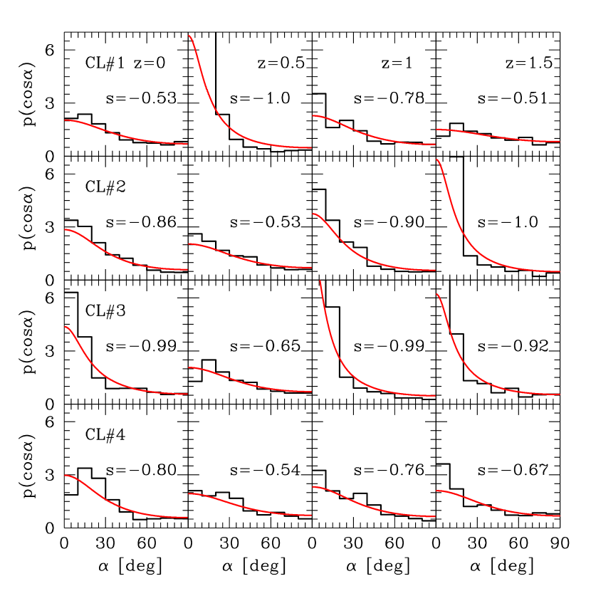
Figure 1: Probability density distributions of the angles between the major axes of four individual host halos and the position vectors of their substructures at four different epochs; $z=0,0.5,1$ and $1.5$. In each panel, the histogram represents the simulation results, and the (red) solid line represent the theoretical prediction (7).

Figure 1 plots the final fitting results. In each panel, the histogram represents the numerically measured $p(\cos\alpha)$, while the (red) solid curve corresponds to the analytic distribution (eq.[7]) with the best-fit correlation parameter, $s$. As one can see, for all cases, the best-fit correlation parameter $s$ has a negative value. In other words, the dark halo substructures are preferentially located near the major axes of their host halos, consistent with previous numerical findings (Knebe et al., 2004; Zentner et al., 2005; Libeskind et al., 2005). Indeed, the analytic distributions agree with the numerical results for all four clusters at all redshifts quite well.

As a final step, we reconstruct the triaxial shapes of the four host halos from their distributions $p(\cos\alpha)$. For this purpose, we adopt the following formula suggested recently by Lee, Jing & Suto (2005):

$$\frac{a_{2}}{a_{1}}=\left(\frac{1-D_{+}\lambda_{2}}{1-D_{+}\lambda_{3}}\right)^{1/2},\qquad\frac{a_{3}}{a_{1}}=\left(\frac{1-D_{+}\lambda_{1}}{1-D_{+}\lambda_{3}}\right)^{1/2}$$ (10)

where $a_{1},a_{2},a_{3}$ represent the three axis lengths of the triaxial host halos in a decreasing order. Equation (10) basically links the two axes ratios of the triaxial host halos to the eigenvalues of the tidal shear tensors. According to this equation, once $\{\lambda_{i}\}^{3}_{i=3}$ is determined, then one can reconstruct the axis-ratios of the host halos.

Equations (8) and (9) allow one to determine the values of $\{\lambda_{i}\}^{3}_{i=3}$ from the best-fit values of $\{\check{\lambda_{i}}\}^{3}_{i=3}$ as

$$\lambda_{1}=\frac{\delta_{c}\check{\lambda_{1}}}{\check{\lambda_{1}}+\check{\lambda_{2}}+\check{\lambda_{3}}},\quad\lambda_{2}=\frac{\delta_{c}\check{\lambda_{2}}}{\check{\lambda_{1}}+\check{\lambda_{2}}+\check{\lambda_{3}}},\quad\lambda_{3}=\frac{\delta_{c}\check{\lambda_{3}}}{\check{\lambda_{1}}+\check{\lambda_{2}}+\check{\lambda_{3}}}$$ (11)

We use $\delta_{c}=1.686$ as an approximation and the best-fit values of $\check{\lambda_{1}},\check{\lambda_{2}},\check{\lambda_{3}}$ to determine the values of $\lambda_{1},\lambda_{2},\lambda_{3}$ using equation (11) for each host halo, and finally reconstruct the axis-ratios of the host halo using equation (10). With the above method, we finally reconstruct the two axis-ratios of all four clusters at four redshifts.

Figure 2 plots the intermediate-to-major axis ratio vs. the minor-to-major axis ratios of the four clusters at four redshifts. In each panel, the (red) triangle dot represents the reconstructed axis-ratios by the above algorithm, and the (blue) square dot is the original axis-ratios from simulations. Although the reconstruction does not look perfect, it works quite satisfactorily, especially given all the approximations used in the algorithm. It is obvious that at least one of the two axis-ratios is fairly accurately reconstructed. We note that for the case of $s\simeq-1$, the difference between $a_{2}/a_{1}$ and $a_{2}/a_{1}$ is relatively large, which trend is also reconstructed well by our algorithm.

4 DISCUSSIONS AND CONCLUSIONS

Our achievements are summarized as follows: (i) we construct an analytic model for the anisotropic spatial distribution of dark halo substructures; (ii) we confirm numerically that the dark halo substructures have a strong propensity to be located near the major axes of their host halos; (iii) we develop an algorithm to reconstruct the triaxial shapes of dark halos from the anisotropic spatial distribution of their substructures.

Successful as are our analytic model and the reconstruction algorithm based on it, it is worth noting a couple of its inconsistencies. First, as mentioned in §2, equation (7) holds only when the tidal shear field is smoothed on the substructure radii. We ignored the smoothing scale difference, which should cause some scatters in the measurement of the correlation parameter $s$. Second, we adopted the spherical collapse condition $\lambda_{1}+\lambda_{2}+\lambda_{3}=\delta_{c}\approx 1.686$ even though we consider triaxial dark matter halos. Definitely, it will be necessary to refine our analytic model further, accounting for these two inconsistencies.

Another limitation of our model is that its underlying assumption has been numerically tested only for the case of the concordance cosmology. Equation (10) was shown to work only provided that the background cosmology is described by the concordance cosmology (Lee, Jing & Suto, 2005). To find the dependence of the correlation parameter, $s$, on cosmology, and to apply the model to a broader range of cosmological models, it will be first necessary to make more general assumptions and to test the underlying assumptions against numerical results, which is definitely beyond the scope of this paper.

Now that we proved that it can reconstruct in principle the axis-ratios of triaxial dark halos from the anisotropic spatial distribution of substructures for the concordance $\Lambda$CDM model, it is worth discussing about how to apply the algorithm to real data from observations of such as the weak gravitational lensing. In our analytic model, the substructure positions are defined in the real three dimensional space relative to the principal axes of host halos, which is, however, very difficult to determine in practice. In observations they are measured in the two dimensional space projected along the line-of-sight direction which is not necessarily coincident with the host halo principal axis. Therefore, to apply our reconstruction algorithm to real data, it will be necessary first to find an analytic expression of the substructure spatial distributions in the general non-principal axis frame and to account for the effect of projection along the line-of-sight. Our future work is in this direction, and we wish to report it elsewhere soon.

Another direction is to explain the Holmberg effect. As shown, our analytic model for the substructure spatial distribution (eq.[7]) is characterized by the single correlation parameter, $s$. By investigating what physical mechanism caused the correlation parameter to change their signs, it might be possible to explain the Holmberg effect theoretically.

Finally, we conclude that our analytic model may provide a physical quantitative understanding of the anisotropic spatial distribution of dark halo substructures, and will allow us to determine in principle the axis-ratios of triaxial dark halos from the observables.

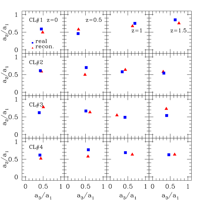
Figure 2: Axis-ratios of four individual clusters at four different epochs; In each panel, the square represents the real axis-ratio measured in simulations while the triangle represents the reconstructed axis-ratio.

References

- Bond (1987) Bond, J. R. 1987, in Nearly Normal Galaxies, ed. S. Faber (New York: Springer), 388
- Bond, Kofman, & Pogosyan (1996) Bond, J., R., Kofman, L., & Pogosyan, D. 1996, Nature, 380, 603
- Brainerd (2005) Brainerd, T. G. 2005, ApJ, 628, L101
- Colless et al. (2001) Colless, M., Dalton, G., Maddox, S., Sutherland, W., & the 2dF collaboration. 2001, MNRAS, 328, 1039
- Eke, Cole, & Frenk (1996) Eke, V., Cole, S., & Frenk, C. 1996, MNRAS, 283, 263
- Fuller, West & Bridges (1999) Fuller, T. M., West, M. J., & Bridges, T. J. 1999, ApJ, 519, 22,
- Hawley & Peebles (1975) Hawley, D. L., & Peebles, P. J. E. 1975, AJ, 80, 477
- Holmberg (1969) Holmberg, E. 1969, Ark. Astron, 5, 305
- Jing & Suto (1998) Jing, Y. P. & Suto, Y. 1998, ApJ, 503, L9
- Jing & Suto (2000) Jing, Y. P. & Suto, Y. 2000, ApJ, 529, L69
- Jing & Suto (2002) Jing, Y. P. & Suto, Y. 2002, ApJ, 574, 538
- Kang et al. (2005) Kang, X., Mao, S., Gao, L., & Jing, Y. P. 2005, A&A, 437, 383
- Knebe et al. (2004) Knebe, A. et al. 2004, ApJ, 603, 7
- Kroupa et al. (2005) Kroupa, P., Theis, C., & Boily, C. M. 2005, A&A, 431, 517
- Lee, Jing & Suto (2005) Lee, J., Jing, Y. P. & Suto, Y. 2005, preprint (astro-ph/0504623)
- Lee, Kang & Jing (2005) Lee, J., Kang, X., & Jing, Y. P. 2005, ApJ, 629, L5
- Lee & Pen (2000) Lee, J. & Pen, U. L. 2000, ApJ, 532, L5
- Lee & Pen (2001) Lee, J. & Pen, U. L. 2001, ApJ, 555, 106
- Libeskind et al. (2005) Libeskind, N. I., Frenk, C. S., Cole, S., Helly, J. C., Jenkins, A., Navarro, J. F., & Power, C. 2005, preprint (astro-ph/0503400)
- Lynden-Bell (1982) Lynden-Bell, D. 1982, Obs., 102, 202
- MacGillivray et al. (1982) MacGillivray, H. T., Dodd, R. J., McNally, B. V., & Corwin, H. G. 1982, MNRAS, 198, 605
- Majewki (1994) Majewki, S. R. 1994, ApJ, 431, L17
- Mo, Mao, & White (1998) Mo, H. J., Mao, S., & White, S. D. M. 1998, MNRAS, 297, L71
- Porciani, Dekel, & Hoffman (2002) Porciani, C., Dekel, A., & Hoffman, Y. 2002, MNRAS, 332, 325
- Sales & Lambas (2004) Sales, L. & Lambas, D. G. 2004, MNRAS, 348, 1236
- Sharp et al. (1979) Sharp, N. A., Lin, D. N. C., & White, S. D. M. 1979, MNRAS, 187, 287
- Springel et al. (2001) Springel, V., White, S. D. M., Tormen, G., Kauffmann, G. 2001, MNRAS, 328, 726
- Strauss et al. (2002) Strass, M. A., Weinberg, D. H., Lupton, R. H., & the SDSS collaboration, 2002, AJ, 124, 1810
- Valtonen et al. (1978) Valtonen, M., Teerikorpi, P., & Argue, A. 1978, AJ, 83, 135
- West (1989) West, M. J. 1989, ApJ, 347, 610
- West (1994) West, M. J. 1994, MNRAS, 268, 79
- Zaritsky et al. (1997) Zaritsky, D., Smith, R., Frenk, C. & White, S. D. M. 1997, ApJ, 478, L53
- Zeldovich (1970) Zel’dovich, Y. B. 1970, A& A, 5, 84
- Zentner et al. (2005) Zentner, A. R., Kravtsov, A. V., Gnedin, O. Y., & Klypin, A. A. 2005, 629, 219