SPITZER VIEW ON THE EVOLUTION OF STAR-FORMING GALAXIES FROM z$=$0 TO z$\sim$3

Abstract

We use a 24 $\mu$m  selected sample containing more than 8,000 sources to study the evolution of star-forming galaxies in the redshift range from $z=0$ to $z\sim 3$. We obtain photometric redshifts for most of the sources in our survey using a method based on empirically-built templates spanning from ultraviolet to mid-infrared wavelengths. The accuracy of these redshifts is better than 10% for 80% of the sample. The derived redshift distribution of the sources detected by our survey peaks at around $z=0.6-1.0$ (the location of the peak being affected by cosmic variance), and decays monotonically from $z\sim 1$ to $z\sim 3$. We have fitted infrared luminosity functions in several redshift bins in the range $0<z\lesssim 3$. Our results constrain the density and/or luminosity evolution of infrared-bright star-forming galaxies. The typical infrared luminosity ($L^{*}$) decreases by an order of magnitude from $z\sim 2$ to the present. The cosmic star formation rate (SFR) density goes as $(1+z)^{4.0\pm 0.2}$ from $z=0$ to $z=0.8$. From $z=0.8$ to $z\sim 1.2$, the SFR density continues rising with a smaller slope. At $1.2<z\lesssim 3$, the cosmic SFR density remains roughly constant. The SFR density is dominated at low redshift ($z\lesssim 0.5$) by galaxies which are not very luminous in the infrared ($L_{\mathrm{TIR}}<10^{11}\,L_{\sun}$, where $L_{\mathrm{TIR}}$ is the total infrared luminosity, integrated from 8 to 1000 $\mu$m). The contribution from luminous and ultraluminous infrared galaxies ($L_{\mathrm{TIR}}>10^{11}\,L_{\sun}$) to the total SFR density increases steadily from $z\sim 0$ up to $z\sim 2.5$, forming at least half of the newly-born stars by $z\sim 1.5$. Ultraluminous infrared galaxies ($L_{\mathrm{TIR}}>10^{12}\,L_{\sun}$) play a rapidly increasing role for $z\gtrsim 1.3$.

1. INTRODUCTION

Infrared surveys are rapidly achieving comparable sample sizes and areal coverage as deep ultraviolet (UV) and optical ones, providing an important perspective on galaxy evolution. Ground-based measurements plus the Infrared Astronomical Satellite (IRAS) have demonstrated that star-forming galaxies are strong infrared sources. Although star formation in disks is also readily detected in the UV or through optical emission-lines, nuclear starbursts are often heavily obscured, making infrared measurements essential to probe them (Kennicutt 1998). Early ground-based photometry (Rieke & Low, 1972) and IRAS (Sanders et al., 1988) also revealed a population of massive galaxies in the local Universe with extremely high rates of star formation ($\mathrm{SFR}>100\,\mathcal{M}_{\odot}\,\mathrm{yr}^{-1}$): the ultraluminous infrared galaxies (ULIRGs). This violent star formation is almost completely undetectable in the optical and UV part of the spectrum due to huge attenuation by dust. Together with lower-luminosity dust-embedded starbursts, this type of activity accounts for up to 20% of the local star formation.

The Infrared Space Observatory (ISO) showed that dust-enshrouded starbursts have undergone strong evolution from $z\sim 1$ to $z=0$ (Franceschini et al., 2001). From results in the sub-mm with SCUBA, it appears that the output of ULIRGs may dominate the energy density in the Universe at $z\geq 2$. However, the limitations in resolution and sensitivity of most of the ISO surveys have not allowed reliable identifications of a sufficient number of infrared galaxies at $z<1$ to estimate robust luminosity functions. The limitations are even more severe for probing the ULIRG population at higher redshifts. At $z\geq 1$, the 8 $\mu$m  polycyclical aromatic hydrocarbons (PAH) band is shifted out of the longest ISOCAM band at 15 $\mu$m, and the longer wavelength ISOPHOT bands have limitations in both sensitivity and angular resolution. Thus, we have only a first-order vision of the importance of infrared-bright galaxies at $0<z<1$ in the general picture of galaxy evolution (e.g., what percentage of the total star formation rate density is contributed by ULIRGs and what for optical/UV selected star-forming galaxies?). We have even less information at $z=1-3$, where we believe the co-moving SFR density reaches a maximum (Somerville et al., 2001; Lanzetta et al., 2002), most of the stars in galaxies were formed (Dickinson et al., 2003; Calura & Matteucci, 2003), and dynamic structures (bars, disks) start to have a role in galaxy evolution (Mo et al., 1998).

Spitzer’s band at 24 $\mu$m  encompasses PAH emission to $z>2$, making star-forming galaxies readily detectable (Egami et al., 2004; Le Floc’h et al., 2004). This band has sensitivity an order of magnitude greater than the ISO $15$ $\mu$m  band, and 16 times as many pixels. Spitzer  also has bands at 70 and 160 $\mu$m, with similar gains over ISO to those at 24 $\mu$m. Spitzer  therefore provides for the first time the ability to survey large fields on the sky to adequate depth to resolve the majority of the far-infrared (FIR) background and to characterize the $z\geq 1$ population of ULIRGs and starbursts. Moreover, MIPS provides a link between the population of objects being discovered in the sub-mm and mm, and the UV/optical and near-infrared (NIR) wavelengths, giving us a key new tool to understand galaxy evolution.

This work is part of a series of papers where we will demonstrate the ability of Spitzer  to unveil galaxy evolution in the $0<z\lesssim 3$ redshift range through its IRAC and MIPS instruments. In Bell et al. (2005) and Papovich et al. (2005) we investigate the processes governing the evolution of star-forming galaxies from $z=0$ to $z\sim 1$. In Le Floc’h et al. (2005), we study the luminosity evolution of infrared-bright sources up to $z\sim 1$ using a sample of sources detected by Spitzer  in the mid-infrared (24 $\mu$m), and the extensive dataset in the Chandra Deep Field South. The paper uses a combination of spectroscopic redshifts and photometric redshifts from the COMBO17 project (Wolf et al., 2004). However, these redshift surveys identify few galaxies at $z\gtrsim 1$. In the present paper, we extend the previously mentioned work to $1<z\lesssim 3$. We develop a photometric technique based on IRAC and deep optical photometry (see Huang et al., 2004; Wilson et al., 2004; Le Floc’h et al., 2004), that is able to obtain reliable redshifts for virtually all the galaxies detected by MIPS up to $z\sim 3$. With these redshifts, we build luminosity functions in the mid-infrared (MIR) in several redshift bins. This will allow us to study the evolution of star-forming galaxies and constrain the SFR history of the Universe up to $z\sim 3$ using a homogeneously selected sample and a SFR estimator not affected by dust attenuation.

This paper is organized as follows. Section 2 presents the observations carried out with Spitzer, and the ancillary data compiled for this study. Section 3 describes the technique used to estimate the redshifts from broad-band photometry for our sample of galaxies. Further details about this technique are given in Appendix A. The main results on the photometric redshifts are presented in Section 4.1. The luminosity function estimation and fitting, constraints on the cosmic star formation rate density, and a discussion of the contribution of galaxies with different SFRs and masses to the total SFR density of the Universe will be presented in Sections 4.2 through 4.5. The method for estimating the luminosity functions, which takes into account the photometric redshift errors, is described in Appendix B. Finally, the conclusions are outlined in Section 5. Throughout this paper, we use a cosmology with $\mathrm{H}_{0}=70$ km s^-1 Mpc^-1, $\Omega_{\mathrm{M}}=0.3$ and $\Lambda=0.7$. All magnitudes refer to the AB system.

2. THE SAMPLE

2.1. Spitzer  observations

The sample used in this paper is drawn from MIPS 24 $\mu$m  observations of the Chandra Deep Field South (CDFS, $\alpha=03^{h}32^{m}02^{s}$, $\delta=-27\arcdeg 37\arcmin 24\arcsec$, J2000) and the Hubble Deep Field North (HDFN, $\alpha=12^{h}37^{m}57^{s}$, $\delta=+62\arcdeg 23\arcmin 14\arcsec$, J2000). In each field, we used the scan map mode to observe a rectangle of $1.5\arcdeg\times 0.5\arcdeg$ in each of the three MIPS wavelengths (24, 70, and 160 $\mu$m). The overlay zone covered with all three channels is $1.0\arcdeg\times 0.4\arcdeg$. To have the most ancillary data for each 24 $\mu$m  selected source, we concentrated this work in a smaller area around the COMBO17 (Wolf et al., 2004), GOODS ACS (Giavalisco et al., 2004b), and ESO Imaging Survey (EIS, Arnouts et al. 2002) pointings in the CDFS case, and around the GOODS ACS footprint in the HDFN. In both fields, we also obtained IRAC data. The CDFS and HDFN were observed in the four IRAC channels (at 3.6, 4.5, 5.8, 8.0 $\mu$m) covering an area of $1.0\arcdeg\times 0.5\arcdeg$ in each field.

The reduction of the 24 $\mu$m  images was carried out with the MIPS Data Analysis Tool (Gordon et al., 2005). The final images had an average exposure time of $\sim 1400$ s. Source detection and photometry were carried out with several tasks (daofind, phot, and allstar) in the DAOPHOT package in the Imaging Reduction and Analysis Facility, IRAF. Sources were detected in two passes to recover the faintest sources, many of which are hidden by brighter ones. Photometry was extracted for all the sources (from the two passes) together to obtain the best possible results in crowded regions. Given the large point spread function (PSF) of the MIPS 24 $\mu$m  channel (which produces very crowded images), all measurements were made by PSF fitting. For sources of noticeable extent, the measurement aperture was set accordingly. For the rest, a circular aperture of size $\sim 15\arcsec$ was utilized. We used an aperture correction based on the theoretical PSF of MIPS to correct to the total flux. The sky estimation was carried out in two steps, first removing the large-scale variation (due to Zodiacal light) and then measuring the background around each source.

IRAC images were reduced with the general Spitzer  pipeline, and then mosaicked. The average exposure time of these frames is approximately 500 s. Source detection and photometry was carried out with SEXTRACTOR (Bertin & Arnouts, 1996), using the same procedure as Huang et al. (2004). Special care was taken with the deblending of sources, given the large density of objects and the marked features of the IRAC PSF. Since the third and fourth IRAC channels are less sensitive than the first and second ones, we tried to obtain fluxes for the faintest sources in the former by carrying out the detection in the latter and measuring photometry in all bands. Photometry was performed using a small circular aperture ($3\arcsec$ in diameter) and an aperture correction was applied to get the total flux (assumed to be the one corresponding to a circular aperture of diameter 24.4$\arcsec$). The aperture corrections were calculated from in-flight PSFs. For extended sources, a circular aperture large enough to capture the total signal was used.

The catalogs for the Spitzer  bands in both the CDFS and HDFN were cut for sky regions where the IRAC/MIPS coverage was the deepest, and other UV/optical/NIR data were available (see next Section). We detected 4373 sources in the CDFS ($4\sigma$ above the sky level) in a area of 665 arcmin²; 4593 sources were detected in the HDFN in 517 arcmin² (above $3\sigma$ of the sky level). In Papovich et al. (2004), we estimated that the final catalogs are 80% complete at $F_{24}=83$ $\mu$Jy.

2.2. Ground based optical and near-infrared photometry

The Spitzer  images were complemented with the extensive dataset available for both the CDFS and HDFN. For the CDFS, we used the publicly available optical images ($UU_{p}BVRI$) released by EIS (Arnouts et al., 2002), the optical fluxes from COMBO17 (Wolf et al., 2004), the $RIz$ frames published by the Las Campanas Infrared Survey (Marzke et al., 1999), the HST/ACS $bviz$ observations carried out by GOODS (Giavalisco et al., 2004b), the near-infrared $JK$ data released by the EIS Deep Public Survey (EIS-DPS, Vandame et al. 2001), $JHK$ frames released by GOODS (Giavalisco et al., 2004b), and the $I$-band photometry and spectroscopic redshifts released by the VIRMOS-VLT Deep Survey (VVDS, Le Fèvre et al. 2004). We also used UV data taken with GALEX in two bands at 150 nm (FUV-band) and 230 nm (NUV-band). For the HDFN, the Spitzer  data were complemented with publicly available ultra-deep optical and NIR data spanning from the $U$- to the $HK_{s}$-band ($UBVRIzHK_{s}$, Capak et al. 2004). We also used the $bviz$ images published by GOODS for the central region in the HDFN. For all these images, source detection and photometry were carried out with SEXTRACTOR (Bertin & Arnouts, 1996). We refer the reader to Appendix A for more detailed information about the data compilation carried out for this paper.

2.3. Redshift ancillary data

Spectroscopic redshifts for 1599 sources have been released by Le Fèvre et al. (2004) for the CDFS (VVDS redshifts). In addition, COMBO17 observed this field with up to 17 medium- and broad-band filters to obtain high quality photometric redshifts (Wolf et al., 2004). For $R<24$, COMBO17 gives redshifts for approximately 11,000 sources. A total of 425 galaxies in our sample in the CDFS have VVDS spectroscopic redshifts (9% of the sample), and 2118 (48%) have COMBO17 photometric redshifts. In the HDFN, several spectroscopic surveys have been or are being carried out. Most of the spectroscopic redshifts have been compiled by the Team Keck Treasury Redshift Survey (TKRS, Wirth et al. 2004) and Cowie et al. (2004). We have also used the photometric redshifts found in Fernández-Soto et al. (1999). Out of the total number of galaxies in the HDFN survey, 601 sources (13%) have a spectroscopic redshift.

2.4. Merged catalogs

Merged catalogs in all the available bands were built by matching the coordinates of the 24 $\mu$m  sources to one (the deepest) reference optical band ($B$ band in the CDFS and $R$ band in the HDFN). A $2\arcsec$ search radius was used. Within this search radius, multiple identifications (i.e., multiple sources in the optical/NIR corresponding to the same 24 $\mu$m  detection) were found for no more than 7% of the sources (in the deepest ground-based images). At this low rate, we do not expect multiple identifications to bias our results.

To measure the photometry, we determined the elliptical aperture (from isophote fitting in the reference band) corresponding to 2.5 times the Kron radius (which contains more than 95% of the total flux of the source, according to Kron 1980). In all cases the apertures were large enough to enclose the PSF profile. This aperture was translated to all the other optical and NIR images. This procedure allowed us to obtain integrated fluxes for each filter in matched apertures, and to estimate the color properly for each source. For sources not detected in the reference image, we used other optical/NIR images as the reference (if possible). In the case of the IRAC and MIPS bands, where the PSF is larger than the object images, the integrated flux was assumed to be that obtained from PSF fitting.

Figure 2.4 shows the 24 $\mu$m  flux distribution of sources in our sample. We also depict the 80% completeness level (83 $\mu$Jy). For fluxes much lower than this value, Papovich et al. (2004) showed that an increasing fraction of the detected sources might be spurious. We tried to identify the real 24 $\mu$m  sources by cross-correlating the MIPS positions with UV-to-MIR catalogs. A simulation of the source density in UV-to-MIR images revealed that for a random position on the sky of the 24 $\mu$m  image, there is a $\sim$20% probability of having a counterpart in one of the bluer bands within the search radius. However, for a 24 $\mu$m  source with identifications in at least three other bands, the probability of a spurious association is almost negligible (less than 3%). Thus, only the 24 $\mu$m  sources detected in three more additional bands were considered as real. Using this criterion, from the 4373 sources selected at 24 $\mu$m  in the CDFS, 4257 (97%) were flagged as non-spurious detections. In the HDFN, we confirmed the detection for 4385 sources (96% of the total 4593 detections). 85% of the possibly spurious sources were below the 83 $\mu$Jy completeness threshold.

MIPS 24 $\mu$m  flux distribution of the sources detected in the CDFS (open histogram limited by a gray line), HDFN (filled gray histogram), and the total survey (open histogram limited by a black line). The 80% completeness flux level is shown at $F_{24}=83$ $\mu$Jy (Papovich et al., 2004).

Of the 4257 sources in the final merged CDFS catalog, 96% were detected by IRAC in at least one channel. The 4% remaining objects were always near very bright sources which interfered with the deblending algorithm. In the HDFN, the percentage is 89% of MIPS sources detected in at least one IRAC channel.

In the optical, an average of $\sim 70$% of the 24 $\mu$m  selected sample is detected down to $B=24.7$, $V=23.8$, $R=23.7$. This percentage rises to almost 90% for $B=25.2$, $V=24.7$, and $R=24.4$ (always using the limiting magnitudes as defined in Appendix A). These statistics mean that 30% of our 24 $\mu$m  selected sample is part of a population of IR-bright sources, starburst or galaxies with active galactic nuclei (AGNs), that are missed by UV/optical deep surveys such as COMBO17. Only with very deep imaging ($R>25$) from large telescopes (8–10 meter class) can we detect these infrared-bright sources. In the NIR, $\sim 30$% of the sources are detected down to $J=22.5$, $K=21.8$ (EIS data). In the UV, 30% of the sample is detected with the GALEX NUV channel, and 14% with the FUV filter.

As mentioned above, our sample selection requires at least four identifications (at 24 $\mu$m  and three more bands). Most MIPS sources are detected in at least one IRAC channel. However, to be included in our sample they typically need to be also detected in at least one optical band . Therefore, extremely red optically faint galaxies, which are expected to reside preferentially at high redshift, may not be included in the sample. However, the number of such optically faint ($R\gtrsim 25$) 24 $\mu$m  sources is at most 3–4% of the total sample (and some of these 24 $\mu$m  sources may be spurious), not large enough to change our results significantly (e.g., the redshift distribution presented in Section 4.1).

3. PHOTOMETRIC REDSHIFT TECHNIQUE

The redshift is one of the most important parameters to understand a distant galaxy. Although it is best determined with spectroscopy, because of the required cost in observing time, photometric methods are increasingly used. Moreover, photometric redshifts are the only approach for very faint samples of galaxies ($R>25$ or $I>24$), given the sensitivity of the currently available spectrographs. There are now a number of works on the technique of photometric redshifts (e.g., Bolzonella et al., 2000; Benítez, 2000; Collister & Lahav, 2004; Wolf et al., 2004), and on the results obtained with them (see, e.g, Lanzetta et al., 1996; Gwyn & Hartwick, 1996; Sawicki et al., 1997; Rowan-Robinson, 2003; Brodwin et al., 2003; Babbedge et al., 2004).

These works fully develop the use of optical and NIR data to obtain photometric redshifts. In this wavelength range, there are a wide variety of spectrophotometric models and templates (e.g., Coleman et al., 1980; Leitherer et al., 1999; Bruzual & Charlot, 2003), which have been tested by many authors and seem to describe accurately the emission from all types of galaxies. Optical methods suffer, however, from dust attenuation, which can have a dramatic effect on the derived photometric redshifts.

Spitzer  surveys have opened another window in the photometric redshift possibilities. First, the galaxies detected by Spitzer  might be very different in their spectral energy distribution (SED) properties from the typical UV/optical and even NIR based surveys. Second, IRAC observations can go much deeper than ground-based NIR ones in a shorter time. Therefore, one can use up to four more NIR and MIR bands along with the optical ones. Although the optical bands often include important redshift indicators, the additional bands increase the confidence in the redshift determinations (Connolly et al., 1997; Rowan-Robinson, 2003). The gain in confidence results largely from the detection of the 1.6 $\mu$m spectral bump (see John 1988; Sawicki 2002; Le Floc’h et al. 2004). An issue is that models have not been developed in the NIR and MIR as thoroughly as in the UV/optical. The reason is twofold: 1) NIR spectroscopy is a relatively new capability (compared to optical); and 2) at these wavelengths, although dust attenuation is almost negligible, dust emission starts to dominate the integrated spectrum of galaxies (in the continuum and in the PAH spectral features). Consequently, one needs detailed radiative transfer calculations to obtain models including both the stellar and dust contributions. Although some progress has been made on this topic (e.g., Corradi et al., 1996; Gordon et al., 1997; Devriendt et al., 1999; Takagi et al., 2003), the set of models available in the literature is far from complete in the description of the emission of all galaxies from the UV to MIR wavelengths.

The lack of a complete and reliable set of models describing the SED properties of galaxies from the UV to the far-infrared and radio wavelengths convinced us to use another approach to the problem. We built empirical broad-band SEDs for galaxies of known redshift (the spectroscopic sample introduced in Section 2.3). The resulting templates were used to fit all the galaxies in the entire sample. If we have a large enough number of previously known redshifts, and if this training set of galaxies is representative of the entire sample, we should be able to obtain reliable redshifts (see Connolly et al., 1995). This method is similar to a neural network technique in the sense that we use the same photometric data (of galaxies with known redshift) to train the photometric redshift algorithm (see Firth et al., 2003; Collister & Lahav, 2004). A detailed description of our photometric redshift technique is given in Appendix A, jointly with a discussion on the reliability of the redshift estimations.

The companion paper by Le Floc’h et al. (2005) provides a different type of test to our redshifts. It is based entirely on well-tested photometric and spectroscopic redshifts up to $z\sim 1.1$. We have compared the results in that paper with those reported here. As will be pointed out at appropriate places in the following sections, the agreement is excellent and demonstrates that the outliers do not bias our results. This agreement substantially increases our confidence in the similar results we obtain at $z>1.1$, where there are few spectroscopic or previous photometric redshifts for our galaxies (see discussion in Appendices A and B).

3.1. Stars

Given the high Galactic latitude of the fields and the MIR selection of the sample, stars were not expected to be detected in our survey in large numbers. In the final catalogs, only 5 sources in the CDFS and 8 in the HDFN were clearly identified with stars (less than 0.1% of the sample), based on the continuously decreasing SED in the NIR and MIR. This result was also checked by studying the STAR_CLASS parameter from SEXTRACTOR for the galaxies detected in the optical/NIR.

3.2. AGNs

Galaxies with an AGN are expected to be bright in the MIR-FIR due to the emission of the hot dust surrounding the central engine (heated by x-ray and UV photons coming from the black hole). Indeed, IR surveys with ISO and Spitzer  are effective in detecting AGNs (Fadda et al., 2002; Franceschini et al., 2002; Alonso-Herrero et al., 2004; Rigby et al., 2004; Lacy et al., 2004). Based on the observed SEDs, we have tried to identify the AGNs (at least the most extreme cases) in our sample by selecting sources with monotonically rising spectra from optical to MIR-FIR wavelengths following a power-law and lacking any spectral feature (as traced by distinguishable changes in the slope of the SED). The MIR-FIR emission of these sources should be dominated by an AGN (Alonso-Herrero et al., 2004; Rigby et al., 2004), and they probably contribute non-negligibly to the bright end of the IR luminosity function. In addition, the photometric redshift estimation for these objects is very uncertain due to the lack of marked spectral features. Given that in this paper we are mainly interested in the evolution of star-forming galaxies, we carried out a first correction for the presence of AGNs in the survey by removing from the sample the sources with monotonically rising spectra (Alonso-Herrero et al., 2005). Approximately 5% of the galaxies in the total sample are within this group. This percentage is lower than the expected fraction of AGNs in MIR-FIR surveys, estimated in the range $10-20$% by several authors based on local samples (Rush et al., 1993), x-ray identifications consistent with an active galaxy (Brandt et al., 2001; Hornschemeier et al., 2001; Fadda et al., 2002; Rigby et al., 2004), and other methods (La Franca et al., 2004). The sources we removed are likely to be the most extreme cases (Type 1 obscured AGNs) within the active galaxy population. The existence of star formation (co-existing with the AGN) contributing significantly to the total IR luminosity of these galaxies is not completely ruled out, but the high dust temperatures necessary to obtain a power-law in the IRAC bands seem to point to a predominant AGN. The luminosity functions and cosmic SFR density calculations in the next Section were obtained from the “AGN-purged” sample. Further analysis of the data will be necessary to estimate the importance of AGNs in Spitzer  surveys with higher reliability.

4. RESULTS

4.1. Redshift distribution

Figure 4.1 shows the redshift distributions for the samples of 24 $\mu$m  selected sources in the CDFS (in red), HDFN (in green), and the total (black). These distributions result from the convolution of the real redshift distribution of galaxies, the errors introduced by the photometric redshift technique, and the (flux dependent) detection curve of our survey. The cosmic variance between the two fields is readily apparent. We find a redshift peak around $z\sim 0.7$ in the CDFS, also seen in the COMBO17 optical survey (Wolf et al., 2004). In the case of the HDFN, there seems to be a density peak at $z\sim 0.6$ and another one at $z\sim 0.9$, which also coincides with what was found by Fernández-Soto et al. (1999) for the WFPC2-HDF original field, and the spectroscopic results obtained by the TKRS team. The apparent widths of these features ($\Delta z\sim 0.3$) support our estimate of the photometric redshift errors. The curve for the total survey shows that the bulk of the sources lie at $0.5<z<1.0$, just in the redshift range that ISO has probed in recent years. However, the enhanced sensitivity of MIPS in comparison with ISO has allowed us to detect a fainter population at $z\lesssim 1.4$ (see discussion below), and a significant number of sources at $1<z<3$. In fact, almost half of the sample lies at $1<z<3$ (43% of the sources in both fields). This is consistent with the results obtained by Le Floc’h et al. (2005) using COMBO17 and VVDS redshifts for MIPS 24 $\mu$m  sources detected in the optical (55% of the sources in the CDFS with $R<24$ lying at $z<1$). Note also that 75% of the sample is located at $0<z<1.4$, for which Figure A.3 and the discussion of it directly confirm the reliability of our photometric redshifts.

Observed redshift distribution for the 24 $\mu$m  selected sources in the CDFS (red) and the HDFN (green). The combined data for both fields and for all flux densities are plotted in black. The predictions according to the models of Chary et al. (2004) and Lagache et al. (2004) for sources with 24 $\mu$m  flux densities larger than 83 $\mu$Jy are plotted in cyan and blue, respectively. The shaded gray area shows the range of results from our work (including the uncertainties in the photometric redshifts) for the 83 $\mu$Jy limit (thus, this distribution is directly comparable with the models).

Figure 4.1 also shows model predictions (cyan and blue histograms) for the 24 $\mu$m  MIPS detections above $F_{24}=83$ $\mu$Jy (Chary et al., 2004; Lagache et al., 2004). These distributions are directly comparable with the gray curve, built from our sample with the sources above the same flux cut (the shaded area depicts the differences in the distribution given by the photometric redshift errors). The general shape of the model distributions is roughly similar to the observations for $z<1$. There are only small differences in the position of the redshift peak, which is in any case strongly affected by cosmic variance, as the curves for the CDFS and the HDFN show. However, the density of sources in each redshift bin below $z=1$ is very different from one model to the other, and from the models to the data presented in this paper. Lagache et al. (2004) predict more sources at low redshift ($z<0.4$) than Chary et al. (2004), and a less marked peak at $z\sim 0.9$. Our data lies between the models, presenting a $15-25$% higher number density than the prediction of Lagache et al. (2004) for $z<1$, and a 50% lower density than what the models by Chary et al. (2004) show at the peak.

The differences between the two models and the data are even larger at $z>1$. According to Chary et al. (2004), very few galaxies should be detected at high redshift. On the contrary, the Lagache et al. (2004) model is bimodal, predicting that half of the infrared bright sources are at $z<1$ and half at $z>1$. The percentage of sources lying at $z>1$ according to our photo-$z$ study (43%) seems to be consistent with this prediction, but most of them are at $z\lesssim 1.5$, whereas the model predicts that most are at $z>1.4$. Lagache et al. (2004) predict a steep decrease in the number of sources detected at $z\sim 1.2$ and a broad maximum around redshift $z=1.8$ with a width of $\Delta z\sim 1.0$. This maximum is caused by prominent PAH features (at wavelengths from 6 to 10 $\mu$m) entering the MIPS 24 $\mu$m  filter as we move to higher redshifts. In contrast, the observed redshift distribution shows a exponential decay with very small and statistically irrelevant peaks at $z>1$. We do not detect the predicted minimum in source counts at $z\sim 1.2$, although this feature could be washed out due to the errors inherent to the photometric redshift technique. The general shape of the observed distribution is closer to the prediction by Chary et al. (2004), although we obtain a substantially higher number density at $z\gtrsim 1.4$.

The uncertainties in photometric redshifts are not able to explain the difference between the Lagache et al. (2004) model and our results at high $z$. The modest portion of redshift outliers expected from our estimates cannot be responsible for the inconsistency, either. Compared with the models, we conclude there is a lower density of sources at high redshift or that the sources that we are detecting at $z>1$ do not present prominent PAH features in the $6<\lambda<10$ $\mu$m  wavelength range (or both). These sources should be very luminous (see Section 4.2, Figure 4.2, and Le Floc’h et al. 2004), and PAH features could be absent or hidden by a bright continuum or by silicate absorption, as some recent luminosity dependent models predict (see, e.g., Chary & Elbaz, 2001; Dale & Helou, 2002). Further analyses of the SEDs of galaxies using the three MIPS wavelengths as well as the ISO bands will be necessary to explore this result.

Number counts at 24 $\mu$m  built for sources in several redshift ranges (not corrected for completeness). Symbols of different colors (joined by dotted lines of the same color for clarity) are used for each redshift range. The continuous lines show the predictions from the Lagache et al. (2004) models for each redshift interval (in the same color as the data points). Black filled stars stand for the total number counts corrected for completeness and presented in Papovich et al. (2004, P04 in the figure).

Papovich et al. (2004), Chary et al. (2004), and Marleau et al. (2004) all presented number counts at 24 $\mu$m. They all found that the peak in the differential number counts was located at a fainter flux ($0.2-0.4$ mJy) than predicted by the models based on ISO 15 $\mu$m  observations (roughly, at 1 mJy). In these papers, it was argued that the difference implies the existence of a previously undetected population of infrared-bright galaxies at $z\sim 1-3$. Using the photometric redshifts derived in this work, we can study the contribution to the number counts of the galaxies in different redshift bins, as shown in Figure 4.1. As we saw in the previous Figure, the Lagache et al. (2004) models underpredict the number of sources at $z<1$, and overpredict the number of galaxies above $z\sim 1$. Our results seem to favor a scenario where there is a strong evolution of infrared-bright sources from $z=0$ to $z\sim 1.0$, and then the evolution decelerates, stops or even inverts (Chary et al., 2004). We will come back to this issue when we present IR luminosity functions in Section 4.3.

4.2. Infrared Luminosities and Star Formation Rates

Models based on IRAS and ISO data on nearby galaxies can be used to estimate the total infrared (TIR, integrated from 8 to 1000 $\mu$m) luminosity (see, for example, Sanders & Mirabel, 1996; Chary & Elbaz, 2001; Dale & Helou, 2002). The most frequently used monochromatic fluxes to estimate TIR luminosities are at 6.7, 12, 15 $\mu$m  (where the highest quality ISO observations were carried out), and also 12, 25, 60, and 100 $\mu$m  (the IRAS bands). Measurements at 12 $\mu$m  have been shown to be a useful estimator of the TIR emission for the luminosity range that we are dealing with ($10^{5}\lesssim L_{\mathrm{TIR}}/L_{\sun}\lesssim 10^{13}$, see Spinoglio & Malkan 1989; Spinoglio et al. 1995; Chary & Elbaz 2001). This conclusion is illustrated in Figure 4.2, where we have plotted the relationship between the monochromatic luminosity at 6.7, 12, and 15 $\mu$m  and the TIR emission according to the models of Chary & Elbaz (2001). This Figure shows that the 6.7 $\mu$m-to-TIR and the 15 $\mu$m-to-TIR correlations present different behaviors for different luminosity ranges. The 12 $\mu$m  data shows the smallest scatter from a linear correlation. Similar results are obtained with other models found in the literature, such as Devriendt et al. (1999) or Dale & Helou (2002).

We estimated TIR luminosities on the basis of the 12 $\mu$m  fluxes for all the sources in the survey. This approach also allowed us to compare with a vast number of papers in the literature based on IRAS 12 $\mu$m  observations of local galaxies. We estimated the rest-frame monochromatic fluxes at 12 $\mu$m  by comparing the observed SEDs with models of MIR-FIR emission. There are several sets of these models available in the literature (e.g., Chary & Elbaz, 2001; Dale & Helou, 2002). All of them combine an IR continuum with PAH emissions. The prominence of these emissions depends on the TIR luminosity of the source. The set of templates span a wide range of TIR luminosities (and, thus, PAH emission properties). However, the models are only distinct for wavelengths redder than $\sim 3$ $\mu$m  in the case of Chary & Elbaz (2001), and 10 $\mu$m  in the case of Dale & Helou (2002), although the observed SEDs in real galaxies actually present very different shapes at bluer wavelengths (see Figures 1 and A.3). We chose the Chary & Elbaz (2001) template set (covering a wider range) and then compared these models with the observed SEDs for rest-frame wavelengths redder than 3 $\mu$m. The 12 $\mu$m  luminosity was assumed to be the one corresponding to the model which best fitted the observed data. For the sources at highest redshift, only one point (the one for the 24 $\mu$m  observation) was available. In this case, we estimated the 12 $\mu$m  luminosity by selecting the model best fitting the luminosity measured by the 24 $\mu$m  channel.

Correlation between the monochromatic luminosity at 6.7, 12, and 15 $\mu$m  and the TIR emission (from 8 to 1000 $\mu$m), according to the models by Chary & Elbaz (2001). The best linear fit to the 12 $\mu$m-to-TIR emission is also plotted (Equation 1).

The equations used to get the TIR emission from the 12 $\mu$m  luminosity (Chary & Elbaz, 2001), and to obtain SFRs from the TIR luminosity (Kennicutt, 1998) are:

$$log(L_{\mathrm{TIR}})=\log(0.89^{+0.38}_{-0.27})+1.094\times\log(L_{\mathrm{12}})$$ (1)

$$\mathrm{SFR}=1.71\times 10^{-10}L_{\mathrm{TIR}}$$ (2)

where all the luminosities are in solar units, and the SFRs in $\mathcal{M}_{\sun}\,\mathrm{yr}^{-1}$.

The estimation of the TIR emission from the monochromatic 12 $\mu$m  luminosity, and the estimation of the 12 $\mu$m  luminosity itself, are subject to uncertainties due to photometric redshift errors and the dispersion of the different models (within the same library and from one library to another; see Papovich & Bell 2002; Le Floc’h et al. 2005). These uncertainties are related to the heterogeneous dust properties observed in galaxies (PAH strength and dust temperature), even for sources with the same bolometric luminosity (Armus et al., 2004). One more caveat in the calculation of the TIR luminosity is the questionable universality of the relationship given in Equation 1, i.e., whether the models derived from data for local galaxies apply to sources at higher redshifts. In this sense, Elbaz et al. (2005) have analyzed a sample of sources observed with both ISOCAM at 15 $\mu$m  and Spitzer  at 24 $\mu$m  and lying at a median redshift of $z\sim 0.7$, obtaining MIR colors that require the presence of PAHs for more than half of their sample. Prominent PAHs have also been detected with IRS in galaxies up to $z\sim 3$ (Houck et al., 2005). Simulations of the observed IRAC color-color diagrams (Sajina et al., 2005) and models of galaxy evolution (Xu et al., 2003; Chary et al., 2004; Lagache et al., 2004) also seem to suggest the presence of PAHs in galaxies at all redshifts. However, as we move to higher redshifts our survey is only able to detect galaxies with high TIR luminosities (LIRGs and ULIRGs, see Figure 4.2). The MIR SEDs of these sources are probably dominated by the continuum emission (Chary & Elbaz, 2001), and consequently the PAH importance should decrease.

Based on all these arguments, we estimate that the 12 $\mu$m  and the TIR luminosities calculated with Equation 1 are accurate within a factor of 2–3 for individual galaxies. In the following discussion, we will avoid conclusions that would be affected by such errors in the TIR luminosities. In future works, it is very desirable to determine better MIR-FIR SEDs of galaxies at different redshifts to improve the monochromatic to TIR relation. In fact, the uncertainty in this correlation will dominate the errors quoted for the luminosities of individual galaxies in the following sections. However, most of the results to come (e.g., the luminosity functions and SFR densities) depend on luminosities averaged over many galaxies. In this case, the net errors should be reduced substantially.

Figure 4.2 shows the TIR luminosities of sources in our survey as a function of redshift (black points). Gray points represent sources with fluxes above the 80% completeness limit (83 $\mu$Jy). A sharp detection limit is seen. Very few galaxies are below this sharp limit, probably most of them being photometric redshift outliers. This plot also shows that we are able to detect galaxies with moderate star formation (starburst galaxies with SFRs of a few $\mathcal{M}_{\sun}\,\mathrm{yr}^{-1}$) up to $z\sim 1$. Very few ULIRGs are detected in this redshift range due to a low number density and/or an insufficient area coverage. Above $z=1$ and up to $z\sim 2$, approximately half of the sources we are detecting present SFRs typical of infrared-luminous galaxies (LIRGs with a few tens $\mathcal{M}_{\sun}\,\mathrm{yr}^{-1}$), and half of them are ULIRGs (SFR$\gtrsim$100 $\mathcal{M}_{\sun}\,\mathrm{yr}^{-1}$). Above $z\sim 2$, the Hyper-luminous infrared galaxy population (HyLIRGs, $L_{\mathrm{TIR}}>10^{13}\,L_{\sun}$ or SFR$\gtrsim$1700 $\mathcal{M}_{\sun}\,\mathrm{yr}^{-1}$) starts to be detected. As expected, at $z\sim 3$ the detection limit reaches only HyLIRGs.

The inset of Figure 4.2 presents the contribution of galaxies with different TIR luminosities to the redshift distribution presented in Figure 4.1. This Figure is not corrected for completeness, i.e., the distributions are affected by the selection effects of our survey. A similar figure accounting for completeness effects is shown in Figure 4.5. The inset of Figure 4.2 shows that starburst galaxies (defined as the ones with $L_{\mathrm{TIR}}<10^{11}\,L_{\sun}$) dominate our survey for redshifts below $z\sim 0.5$, and are not detected beyond $z\sim 1$. The distribution for LIRGs shows a clear evolution from $z=0$, where very few are detected, to $z\sim 0.4$, where the number of detected LIRGs starts to rise rapidly. At $z\sim 1$, all the sources in the survey are LIRGs. The curve for ULIRGs clarifies the statement in the previous paragraph about the dominance in our survey of this kind of sources at $z>2$.

Selection effect on TIR luminosities of our 24 $\mu$m  survey for the entire sample (black stars) and sources with flux above 83 $\mu$Jy (gray stars). The divisions for LIRGs ($10^{11}<L_{\mathrm{TIR}}<10^{12}\,L_{\sun}$), ULIRGs ($10^{12}<L_{\mathrm{TIR}}<10^{13}\,L_{\sun}$), and HyLIRGs ($L_{\mathrm{TIR}}>10^{13}\,L_{\sun}$) are marked with horizontal lines. The inset plot shows the redshift distribution of sources with flux above 83 $\mu$Jy divided into three luminosity ranges: starbursts ($L_{\mathrm{TIR}}<10^{11}\,L_{\sun}$), LIRGs ($10^{11}<L_{\mathrm{TIR}}<10^{12}\,L_{\sun}$), and ULIRGs ($L_{\mathrm{TIR}}>10^{12}\,L_{\sun}$).

4.3. Mid-infrared Luminosity functions

We constructed and fitted luminosity functions at 12 $\mu$m  to study the evolution of the total infrared output of the population of galaxies as a function of redshift, and to put constraints on the evolution of parameters such as the typical TIR luminosity of galaxies ($L^{*}$). The luminosity functions are weakly constrained at the highest redshifts. Toward low luminosities, the achievable sensitivity becomes an increasingly severe limitation, while our surveyed area is inadequate to include rare, very high-luminosity objects. To estimate the resulting systematic errors, we have used a variety of approaches to fit luminosity functions to the data. First, we fitted a standard form of luminosity function, allowing parametric adjustment of the density normalization, the slope at faint luminosities, and $L^{*}$ to minimize a $\chi^{2}$ likelihood estimator. Second, we used a variety of functional forms determined for nearby galaxies and forced fits to the data at different redshifts. We were careful in selecting the various fitting approaches to include cases that would provide upper and lower limits to the TIR luminosity density of the galaxy population, allowing us to test our conclusions.

For all the luminosity function construction, we divided the sample into redshift bins selected to provide adequate numbers of galaxies to constrain the fits well. For $0<z<1$, we used five equal intervals ($\Delta z=0.2$). We used four additional intervals for $1<z<2.6$ ($\Delta z=0.4$). No estimations were made for $z>2.6$, given the small range of luminosities in our sample at such high redshift. The estimation of the luminosity function was carried out using a stepwise maximum-likelihood technique (SWML, Efstathiou et al., 1988, see also Willmer 1997), modified to take into account the uncertainties in the photometric redshifts. The procedure is described in Appendix B (see also Chen et al., 2003). The results were also checked using the $V/V_{\mathrm{max}}$ method (Schmidt, 1968; Huchra & Sargent, 1973).

Once we had estimated the luminosity functions with the modified SWML method, we carried out a variety of fits (see Figures 4.3 and 4.3). For the parametric fitting (SCHLF fit from now on), we used a Schechter (1976) function because it includes only three free parameters (normalization $\phi^{*}$, faint-luminosity slope $\alpha$, and typical luminosity $L^{*}$), in comparison with the four parameters in other parametrizations (such as a double power-law). Each fit at each redshift interval was independent from the others.

The Schechter parametrization is commonly used for UV/optical luminosity functions. In our case, it fits the data points well for $z>0.2$ with a minimum of free parameters. It is likely that the true luminosity function is more similar to a double power-law, as many authors have shown for the local infrared galaxy population (Lawrence et al., 1986; Saunders et al., 1990; Rush et al., 1993; Serjeant et al., 2001; Takeuchi et al., 2003, among others). Our results in the local Universe also seem to fit better to a double power-law, once you complement them with the data from other works at the bright-end (see Figures 4.3 and 4.3 and the discussion below). However, within the limited luminosity range of our data for $z>0.2$ (where we can only estimate the number density of sources for $L_{TIR}\gtrsim 10^{9}\,L_{\sun}$), there is little difference between a Schechter curve and a double power-law. The extra parameter required in the double power-law is therefore not well justified for our fits.

We also carried out a second set of fits, using two forms of double power-law functions : 1) we used the local luminosity function derived by Rush et al. (1993); this fit (RUSHLF fit from now on) presents a much steeper faint-end slope than the local SCHLF, and a less steep slope at high luminosities (see Figure 4.3 and the discussion of it); and 2) we used our own derivation of the local luminosity function (OWNLF from now on), that presents an almost flat faint-end slope (very similar to the SCHLF one) and is practically identical to the local RUSHLF at high luminosities (see the discussion below). The comparison of the three different fits to the data lets us test directly the contribution of high luminosity galaxies to the overall luminosity density of the population. With the high luminosity shape fixed at the double power-law fit, the results as a function of $\alpha$ also let us test the contribution of low infrared luminosity galaxies to the overall output of the population. The probed values of $\alpha$, from $\alpha=-1.7$ corresponding to the local RUSHLF fit to $\alpha\sim-1.0$ corresponding to the SCHLF or to our OWNLF fit, are typical for local infrared-selected galaxies (Rush et al., 1993; Fang et al., 1998; Xu et al., 1998; Pozzi et al., 2004). This range is also very similar to the values found at other wavelengths for different SFR estimators and at different redshifts (see Hopkins 2004 and references therein, and also Cohen 2002, Poli et al. 2003, Bouwens et al. 2004, and Gabasch et al. 2004a, b).

Most contemporary models of galaxy evolution assume that the observed change of the infrared luminosity function with redshift can be expressed through a number density and/or a luminosity evolution of the local luminosity function. This means that the shape of the luminosity function is conserved. The evolution is normally parametrized with a $(1+z)^{n}$ law affecting the vertical axis (number density), and another power-law making the luminosity function slide along the horizontal axis (luminosity evolution). In the double power-law set of fits, we allowed either a pure luminosity evolution (of the local luminosity function) following a $(1+z)^{n_{L}}$ law ($L$ case), or a pure number density evolution following a $(1+z)^{n_{D}}$ law ($D$ case), or a combination ($L+D$ case), to test the dependencies of the results on the assumed evolutionary behavior. The results of the different fits are illustrated in Figures 4.3 through 4.5. The recovered luminosity function parameters jointly with the derived luminosity densities $\rho_{L_{12}}$ (for each set of fits) are given in Tables 1 and 2.

Local luminosity function at 12 $\mu$m  estimated by several authors using IRAS, ISO, and Spitzer data. Black filled stars show the results from this work (obtained with the entire sample of galaxies in the CDFS and the HDFN). Error bars are the associated 1-$\sigma$ uncertainties based on Poisson statistics (Schechter, 1976) and the propagation of photometric redshift errors (see Appendix B). Our results are compared with those achieved with IRAS data (for non-active galaxies) by Rush et al. (1993, blue open stars) and those obtained with ISO observations by Pozzi et al. (2004, cyan crossed circles). The best fit of our results to a Schechter (1976) function is plotted in red, the fit to two power-laws (including the points from Rush et al. 1993 at $L_{12}>10^{10}\,L_{\odot}$) is plotted in black (in both cases, taking into account the luminosity function errors), and the double power-law fit given by Rush et al. (1993) is plotted in blue.

Figure 4.3 shows the local 12 $\mu$m  luminosity function built with all the galaxies in our CDFS and HDFN surveys and the best fits to it. Our results are compared with those obtained by Rush et al. (1993) using IRAS data and those achieved by Pozzi et al. (2004) using ISO observations (see also Fang et al., 1998; Xu et al., 1998). Given that we only detect one galaxy with $L_{12}>10^{10}\,L_{\sun}$, we assumed Rush et al. points in this regime to obtain the OWNLF fit. For luminosities $10^{8}\lesssim L_{12}\lesssim 10^{10}\,L_{\sun}$, our results are very close to the IRAS estimation, which presents slightly larger number densities than ISO. For $L_{12}\lesssim 10^{8}\,L_{\sun}$, our results are consistent with a rather flat luminosity function down to $L_{12}\sim 10^{6.5}\,L_{\sun}$, and even below, in contrast to the IRAS results. We find $\alpha=-1.23\pm 0.06$ for the SCHLF fit ($\alpha=-1.17\pm 0.07$ for the OWNLF fit), which is very close to the results obtained for the local luminosity function of star-forming galaxies using other SFR estimators (see, e.g., Serjeant et al. 2002, Pérez-González et al. 2003c, Wyder et al. 2005, Budavári et al. 2005, and also Figure 4.3).

Figure 4.3 shows the 12 $\mu$m  luminosity functions for all the galaxies in our CDFS and HDFN surveys in the nine redshift bins mentioned above (including the local function, plotted with a smaller scale than in Figure 4.3), and the fits to the data. These fits illustrate one consequence of our choice of the Schechter function: the contribution at high luminosities is minimized compared with the more plausible double power-law fits. Thus, the SCHLF fits most probably underestimate the overall infrared output from high luminosity galaxies, while the RUSHLF and OWNLF approaches seem to provide better fits in this regime. A more subtle effect is that the slope toward low luminosities is not well constrained, although it seems to remain at a rather flat value ($-1.2\gtrsim\alpha\gtrsim-1.0$) according to the SCHLF fits and in good agreement with the OWNLF local value. The RUSHLF case provide the worst fits of the three sets, given that it assumes a very steep value of $\alpha$. However, the small values of the slope may result from incompleteness in the lowest luminosity bin fitted, plus the poor coverage toward low luminosities in general. Thus, it is possible that we are underestimating the number density of faint sources (i.e., the $\alpha$ parameter). In the following Section, the effect of the large uncertainties in the faint-end slope on the estimation of the total luminosity density will be investigated by comparing the two extreme cases: 1) $\alpha\sim-1$ for the SCHLF or OWNLF fits, either of which must provide a lower limit to the total output of the population of galaxies in each redshift bin; and 2) $\alpha\sim-1.7$ in the RUSHLF case, which must provide an upper limit for the luminosity density, with an important contribution from low luminosity sources.

The most robust result of the SCHLF fits is the steady growth of $L^{*}$ with increasing redshift. This is shown in Figure 4.3 (red stars), jointly with the evolution of the other luminosity function parameters for each set of fits. The normalization parameter, $\phi^{*}$, grows slowly (or perhaps it is nearly constant, see the discussion below) to $z\sim 0.8$, and then it seems to fall. This observed decrease of $\phi^{*}$ at $z\gtrsim 1$, which seems to be also found by other authors using Schechter fittings to luminosity functions of star-forming galaxies built at other wavelengths (cf. gray crosses in Figure 4.3), may be strongly influenced by the poor coverage at low luminosities, so it should be regarded with caution. We will come back to this issue later. The fitting errors in the slope parameter are large, and even without appealing to incompleteness, values of $\alpha\sim-1.2$ are consistent with the data (and compatible with other estimations of the luminosity function of star-forming galaxies, cf. gray crosses in Figure 4.3). Since the Schechter function is also expected to underestimate the number of high-luminosity infrared galaxies, the parametric fits are generally consistent with the forms of the luminosity function found locally.

Luminosity functions at 12 $\mu$m  for galaxies in several redshift ranges for both the CDFS and HDFN (black filled stars in all the panels). For the sake of completeness and clarity, we reproduce the 12 $\mu$m  local luminosity function given in Figure 4.3 using smaller scales. The best fit to a Schechter (1976) function is plotted in red, the fit to two power-laws given by Rush et al. (1993) is plotted in blue, and our own double power-law fit is plotted in green (all with dot-dashed lines). The three fits of the local luminosity function are also shown in all the other panels (with the same color and line style). The continuous lines in the other panels show the best fits for each of the approaches described in the text: independent fit to a Schechter function (SCHLF), evolution of the local luminosity function given by Rush et al. (1993, RUSHLF), and evolution of the local luminosity function obtained in this work (OWNLF). Red continuous lines show the best SCHLF fit. Blue continuous lines show the best RUSHLF fit for each redshift interval after applying a density plus luminosity evolution. Green continuous lines show the best OWNLF fit for each redshift interval after applying a density plus luminosity evolution. Note that a pure luminosity evolution would give practically the same results (i.e., we are not able to break the degeneracy between the pure luminosity and the density plus luminosity evolution).

Table 1Results of the Schechter (1976) fits (SCHLF) to the 12 $\mu$m  luminosity functions.

	$\alpha_{12}$	$\log(L^{*}_{12})$	$\log(\phi^{*}_{12})$	$\log(\rho_{L_{12}})$
Redshift range		$[L_{\odot}]$	$[\mathrm{Mpc}^{-3}\,\mathrm{Mag}^{-1}]$	$[L_{\odot}\mathrm{Mpc}^{-3}]$
$0.0<z\leq 0.2$	$-1.23\pm 0.07$	0$9.61\pm 0.14$	$-2.31\pm 0.16$	$7.38\pm 0.06$
$0.2<z\leq 0.4$	$-1.17\pm 0.08$	0$9.81\pm 0.05$	$-2.18\pm 0.07$	$7.68\pm 0.02$
$0.4<z\leq 0.6$	$-1.05\pm 0.14$	$10.05\pm 0.06$	$-2.09\pm 0.08$	$7.98\pm 0.03$
$0.6<z\leq 0.8$	$-1.03\pm 0.12$	$10.17\pm 0.04$	$-2.10\pm 0.05$	$8.08\pm 0.02$
$0.8<z\leq 1.0$	$-1.06\pm 0.46$	$10.52\pm 0.11$	$-2.37\pm 0.17$	$8.17\pm 0.23$
$1.0<z\leq 1.4$	$-1.16\pm 0.15$	$10.73\pm 0.05$	$-2.50\pm 0.08$	$8.28\pm 0.03$
$1.4<z\leq 1.8$	$-1.15\pm 0.34$	$11.04\pm 0.10$	$-2.85\pm 0.09$	$8.24\pm 0.04$
$1.8<z\leq 2.2$	$-1.05\pm 0.55$	$11.54\pm 0.25$	$-3.38\pm 0.20$	$8.17\pm 0.12$
$2.2<z\leq 2.6$	$-1.05\pm 0.34$	$11.86\pm 0.25$	$-3.58\pm 0.18$	$8.29\pm 0.11$

Table 2Results of the fits to an evolved local luminosity function of the 12 $\mu$m  luminosity functions.

		RUSHLF1				OWNLF2
	Evol.3	$\log(L^{*}_{12})$	$\log(\phi^{*}_{12})$	$\log(\rho_{L_{12}})$		$\log(L^{*}_{12})$	$\log(\phi^{*}_{12})$	$\log(\rho_{L_{12}})$
Redshift range		$[L_{\odot}]$	$[\mathrm{Mpc}^{-3}\,\mathrm{Mag^{-1}}]$	$[L_{\odot}\mathrm{Mpc}^{-3}]$		$[L_{\odot}]$	$[\mathrm{Mpc}^{-3}\,\mathrm{Mag^{-1}}]$	$[L_{\odot}\mathrm{Mpc}^{-3}]$
$0.0<z\leq 0.2$	$L$	0$9.90\pm 0.05$	$-3.10\pm 0.07$	$7.34\pm 0.06$		0$9.33\pm 0.09$	$-2.19\pm 0.10$	$7.36\pm 0.06$
	$L+D$	0$9.90\pm 0.05$	$-3.10\pm 0.07$	$7.34\pm 0.06$		0$9.33\pm 0.09$	$-2.19\pm 0.10$	$7.36\pm 0.06$
$0.2<z\leq 0.4$	$L$	$10.24\pm 0.07$	$-3.10\pm 0.07$	$7.66\pm 0.03$		0$9.59\pm 0.10$	$-2.19\pm 0.10$	$7.57\pm 0.02$
	$L+D$	$10.09\pm 0.06$	$-2.95\pm 0.09$	$7.65\pm 0.02$		0$9.55\pm 0.10$	$-2.14\pm 0.10$	$7.62\pm 0.02$
$0.4<z\leq 0.6$	$L$	$10.54\pm 0.12$	$-3.10\pm 0.07$	$8.04\pm 0.05$		0$9.81\pm 0.12$	$-2.19\pm 0.10$	$7.87\pm 0.03$
	$L+D$	$10.25\pm 0.09$	$-2.82\pm 0.12$	$8.03\pm 0.04$		0$9.73\pm 0.11$	$-2.11\pm 0.11$	$7.85\pm 0.03$
$0.6<z\leq 0.8$	$L$	$10.79\pm 0.16$	$-3.10\pm 0.07$	$8.21\pm 0.06$		$10.01\pm 0.14$	$-2.19\pm 0.10$	$8.02\pm 0.03$
	$L+D$	$10.39\pm 0.12$	$-2.70\pm 0.15$	$8.21\pm 0.04$		0$9.90\pm 0.13$	$-2.07\pm 0.13$	$8.04\pm 0.02$
$0.8<z\leq 1.0$	$L$	$10.85\pm 0.20$	$-3.10\pm 0.07$	$8.29\pm 0.24$		$10.11\pm 0.17$	$-2.19\pm 0.10$	$8.15\pm 0.24$
	$L+D$	$10.61\pm 0.15$	$-2.84\pm 0.18$	$8.31\pm 0.24$		$10.16\pm 0.15$	$-2.24\pm 0.14$	$8.15\pm 0.23$
$1.0<z\leq 1.4$	$L$	$10.93\pm 0.25$	$-3.10\pm 0.07$	$8.36\pm 0.10$		$10.23\pm 0.20$	$-2.19\pm 0.10$	$8.26\pm 0.06$
	$L+D$	$10.74\pm 0.19$	$-2.86\pm 0.22$	$8.42\pm 0.07$		$10.35\pm 0.17$	$-2.37\pm 0.16$	$8.20\pm 0.04$
$1.4<z\leq 1.8$	$L$	$11.02\pm 0.30$	$-3.10\pm 0.07$	$8.46\pm 0.12$		$10.38\pm 0.24$	$-2.19\pm 0.10$	$8.41\pm 0.07$
	$L+D$	$11.28\pm 0.23$	$-3.47\pm 0.27$	$8.35\pm 0.08$		$10.82\pm 0.21$	$-2.86\pm 0.18$	$8.18\pm 0.04$
$1.8<z\leq 2.2$	$L$	$11.17\pm 0.35$	$-3.10\pm 0.07$	$8.60\pm 0.18$		$10.55\pm 0.28$	$-2.19\pm 0.10$	$8.58\pm 0.14$
	$L+D$	$12.08\pm 0.27$	$-4.23\pm 0.31$	$8.38\pm 0.15$		$11.33\pm 0.24$	$-3.36\pm 0.20$	$8.19\pm 0.12$
$2.2<z\leq 2.6$	$L$	$11.42\pm 0.39$	$-3.10\pm 0.07$	$8.86\pm 0.18$		$10.80\pm 0.31$	$-2.19\pm 0.10$	$8.83\pm 0.13$
	$L+D$	$12.21\pm 0.30$	$-4.18\pm 0.35$	$8.56\pm 0.15$		$11.63\pm 0.26$	$-3.46\pm 0.22$	$8.39\pm 0.11$

Note. — ¹ For the RUSHLF fits, the slopes at low and high luminosities are fixed: $\alpha_{12}=-1.70\pm 0.02$ and $\beta_{12}=-3.60\pm 0.09$. ² For the OWNLF fits, the slopes are also fixed: $\alpha_{12}=-1.17\pm 0.07$ and $\beta_{12}=-2.97\pm 0.16$. ³The type of evolution can be: luminosity evolution ($L$), or a combined luminosity plus number density evolution ($L+D$).

For the RUSHLF and OWNLF fits, the growth of $L^{*}$ with redshift is again a robust result, as shown by the green and blue stars in the first panel of Figure 4.3 . This result is obtained for both pure luminosity evolution (open stars) and combined luminosity plus density evolution (filled stars), although the rate of change varies from one type of evolution to the other (and from these to the SCHLF approach). The rate of change from $z=0$ to $z\sim 1$ seems to follow a $(1+z)^{n_{L}}$ law, where $n_{L}=3-5$. In the region of overlap ($z\lesssim 1.1$), this behavior agrees closely with the results of Le Floc’h et al. (2005). The uniform pure density evolution seems to be ruled out by our data, given that it fails to describe the luminosity function points as early as $z\sim 0.4$. Indeed, the probability of exceeding by chance the $\chi^{2}$ value obtained for the fit with a pure density evolution is 7% for the RUSHLF fits (5% for OWNLF). In contrast, the probability of exceeding by chance the $\chi^{2}$ value obtained for the fit with pure $L$ or $L+D$ evolution is 75% (80%) and 90% (93%), respectively. This means that we are not able to confidently break the degeneracy between these two scenarios, although the fits for the combined $L+D$ evolution are slightly better. That is, the luminosity function data points can be reproduced with a strong $L$ evolution ($n_{L}\sim 4-5$), or with a weaker luminosity evolution ($n_{L}=2.6-3.1$) combined with a relatively smaller density evolution ($n_{D}=0.5-2.0$). When we used Schechter functions, which also allowed changes in the faint end slope, the combined $L+D$ evolution is also slightly favored.

Figure 4.3 also shows the best linear fits to the evolution of the luminosity function parameters at $0<z<0.8$. In the case of the Schechter fitting, the number density of sources, as parameterized by $\phi^{*}$, evolves as $(1+z)^{0.9\pm 0.6}$ in this redshift range. The typical infrared luminosity ($L^{*}$) evolves as $(1+z)^{3.1\pm 0.5}$. In the OWNLF fits, the $L+D$ evolution predicts $L^{*}\propto(1+z)^{3.0\pm 0.3}$ and $\phi^{*}\propto(1+z)^{0.6\pm 0.2}$ (green dashed lines in the first two panels). In comparison, when we fit the data with a pure $L$ evolution in the OWNLF case, $\phi^{*}$ remains obviously constant, and $L^{*}$ behaves similarly to the Schechter function fits, evolving as $(1+z)^{3.6\pm 0.3}$ (green dotted lines in the first two panels). As we mentioned before, the RUSHLF fits are always considerably worse than the OWNLF and SCHLF ones, but they predict similar evolution laws: $L^{*}\propto(1+z)^{2.6\pm 1.1}$ and $\phi^{*}\propto(1+z)^{2.1\pm 0.6}$ for the $L+D$ case, and $L^{*}\propto(1+z)^{4.7\pm 0.3}$ for the pure $L$ evolution. Combining the results from the three sets of fits, the most probable values of the exponents of the evolution laws are: $n_{L}=3.0\pm 0.3$ and $n_{D}=1.0\pm 0.3$.

Above $z\sim 0.8$, the evolution degeneracy is more severe. The Schechter fits seem to favor a scenario where $\phi^{*}$ decreases steadily as $(1+z)^{-5.1+0.8}$, and $L^{*}$ continues rising as $(1+z)^{4.8\pm 0.8}$, i.e., a few galaxies with very violent star formation dominate the TIR luminosity density. However, our data could also be reproduced with a slower (or even null) decrease of $\phi^{*}$ up to $z\sim 3$ and an also slower increase of $L^{*}$ (see open stars in the left two panels of Figure 4.3).

Evolution of the 12 $\mu$m  luminosity function parameters from $z=0$ to $z\sim 3$. For all panels, the results from the SCHLF, RUSHLF, and OWNLF fits are plotted in red, blue, and green, respectively. Open stars refer to the results for a pure luminosity ($L$) evolution, while filled stars refer to a combined luminosity plus density evolution ($L+D$). The best fits for the evolution of $\L^{*}$ and $\phi^{*}$ at $z<0.8$ are plotted with dotted and dashed lines for $L$ and $L+D$ evolutions, respectively, with the same color code as the points for the three sets of fits. Gray symbols show some comparison values for the three parameters (for a Schechter parametrization) extracted from the literature and based on fits of luminosity functions built with samples of star-forming galaxies selected with different SFR estimators (Gallego et al. 1995; Connolly et al. 1997; Tresse & Maddox 1998; Cowie et al. 1999; Steidel et al. 1999; Yan et al. 1999; Machalski & Godlowski 2000; Moorwood et al. 2000; Hopkins et al. 2000; Sullivan et al. 2000; Wilson et al. 2002; Gallego et al. 2002; Sadler et al. 2002; Serjeant et al. 2002; Tresse et al. 2002; Teplitz et al. 2003; Pérez-González et al. 2003c; all these estimations were compiled by Hopkins 2004, from which we extracted the SFR calibrations to convert all the $L^{*}$ values based on different estimators to $L_{12}^{*}$). The evolution laws plotted in the Figure for a $L+D$ scenario are: $L^{*}$ evolves as $(1+z)^{3.1\pm 0.5}$ and $\phi^{*}$ evolves as $(1+z)^{0.9\pm 0.6}$ for the SCHLF fitting (red dashed lines); $L^{*}\propto(1+z)^{2.6\pm 1.1}$ and $\phi^{*}\propto(1+z)^{2.1\pm 0.6}$ for RUSHLF (blue dashed lines); and $L^{*}\propto(1+z)^{3.0\pm 0.3}$ and $\phi^{*}\propto(1+z)^{0.6\pm 0.2}$ for the OWNLF case (green dashed lines). For a pure $L$ evolution: $L^{*}\propto(1+z)^{4.7\pm 0.3}$ for RUSHLF (blue dotted line); and $L^{*}\propto(1+z)^{3.6\pm 0.3}$ for OWNLF (green dotted line).

4.4. Cosmic star formation rate density

In the previous Section, we presented two ways of fitting the luminosity functions: one using a Schechter function to fit the data independently at each individual redshift range, and the other assuming a constant shape of the luminosity function (the local shape, which is the best constrained) and evolving it with redshift in density or/and luminosity. The former technique allows a change in the shape of the luminosity function, mostly in the faint end slope, while the latter procedure fixes this slope. It also assumes a less rapid fall at high-luminosities, which seems to be the case in the local Universe. In this Section, we integrate the SCHLF, OWNLF, and RUSHLF fits of the luminosity functions to get different (possibly biased) estimates of the total 12 $\mu$m  luminosity density of the Universe at $0<z\lesssim 3$, the TIR luminosity density, and the SFR density. The TIR luminosities have been estimated using Equation 1. These luminosity densities will be translated to cosmic SFR densities in Figure 4.4 using Equation 2. At the end of this Section, by comparing the results obtained with the three sets of fits, we will discuss how changes in the faint end and bright end slopes affect the estimations of the luminosity and SFR densities.

The Lilly-Madau diagram (Lilly et al., 1995; Madau et al., 1996): evolution of the SFR density of the Universe with redshift. The estimations based on the SCHLF, RUSHLF, and OWNLF fits are plotted with red, blue, and green stars, respectively (see text for details). The shaded area delimits the zone between the two extreme SFR density estimations for each redshift. The heavy error bar at $z\sim 0.1$ shows the uncertainty in the transformation from the monochromatic 12 $\mu$m  luminosity to the TIR emission, as shown in Equation 1 (see the text for a discussion of this error). This error is common for all our points, but it is only given in the first one for clarity. Vertical segments for each point show the uncertainty related to the integration of the SCHLF luminosity function (comparable to the OWNLF and RUSHLF cases). The horizontal lines show the range of redshifts used in each bin. The curves show two typical models: one with a decay from $z\sim 1$ (Xu et al., 2003, S1 model), and another with a constant SFR density at high redshift (Lagache et al., 2004). The colored points (shown with error bars) are extracted from different sources in the literature, normalized to the same cosmology by Hopkins (2004). Red symbols are estimations based on H$\alpha$ or H$\beta$ measurements (Gallego et al., 1995; Pettini et al., 1998; Tresse & Maddox, 1998; Glazebrook et al., 1999; Yan et al., 1999; Moorwood et al., 2000; Hopkins et al., 2000; Sullivan et al., 2000; Tresse et al., 2002; Pérez-González et al., 2003c). Green symbols stands for $[OII]\lambda 3737$ estimations (Hammer et al., 1997; Hogg et al., 1998; Gallego et al., 2002; Teplitz et al., 2003). UV-based data points are plotted in blue (Lilly et al., 1996; Connolly et al., 1997; Treyer et al., 1998; Cowie et al., 1999; Steidel et al., 1999; Sullivan et al., 2000; Massarotti et al., 2001; Wilson et al., 2002; Giavalisco et al., 2004a). Cyan estimations are based on mid-infrared data (Flores et al., 1999). Magenta points are based on sub-mm and radio observations (Condon, 1989; Hughes et al., 1998; Barger et al., 2000; Machalski & Godlowski, 2000; Haarsma et al., 2000; Sadler et al., 2002; Serjeant et al., 2002; Condon et al., 2002). The yellow point is based on X-ray data (Georgakakis et al., 2003).

Figure 4.4 shows the evolution of the SFR density of the Universe as a function of redshift (red, green, and blue stars referring to the integration of the SCHLF, OWNLF, and RUSHLF fits, respectively) in a Lilly-Madau diagram (Lilly et al., 1995; Madau et al., 1996). Our survey reproduces the rapid increase in $\rho_{\mathrm{SFR}}$ from $z=0$ to $z\sim 1.4$ observed by many previous works. Our estimations follow a $(1+z)^{4.0\pm 0.2}$ law up to $z=0.8$ (i.e., $\beta=4.0\pm 0.2$), and a lower slope ($\beta\sim 3.4$) up to $z\sim 1.4$. For $z<1$, we obtain:

$$\log{(\rho_{\mathrm{SFR}})}=(-1.87\pm 0.04)+(3.98\pm 0.22)\times\log{(1+z)}$$ (3)

This result is consistent with that of Hopkins (2004, see also ), who used all the SFR density estimations plotted in Figure 4.4 (obtained with different SFR tracers), although our slope is higher (and our local density is slightly smaller): Hopkins (2004) gives $\beta=3.10\pm 0.25$ applying a simple obscuration correction for the SFR density estimations, and $\beta=3.29\pm 0.26$ for a luminosity-dependent obscuration correction. The analysis of Hopkins (2004) is partly based on UV surveys, which tend to obtain significantly less steep values of the SFR density evolution slope ($\beta=2-2.5$, see Schiminovich et al. 2005; Baldry et al. 2005). However, other works based on UV and optical surveys (using different emission-lines) find larger values, closer to our estimation (e.g., Lilly et al. 1996; Tresse et al. 2002; Hippelein et al. 2003). Moreover, models based on IR and sub-millimeter models also predict an evolution with an exponent close to $\beta\sim 4$ (Blain et al., 1999; Xu et al., 2003; Lagache et al., 2004).

The scatter in the results for the slope of the evolution of $\rho_{\mathrm{SFR}}$ suggests that the extinction properties of the galaxies dominating the total SFR density are evolving with redshift. For example, our estimation of the SFR density at $z\sim 0.1$ (which is consistent with other estimations based on radio observations, e.g., Condon 1989; Sadler et al. 2002; Serjeant et al. 2002) is $\sim$40% lower than the most recent results achieved by $H\alpha$ (Pérez-González et al., 2003c) or UV/optical surveys (Glazebrook et al., 2003; Wyder et al., 2005; Schiminovich et al., 2005; Martin et al., 2005) in the local Universe. This may indicate that the star formation in this redshift regime is dominated by galaxies with not very extincted bursts, where the dust emission only traces a small part of the total SFR of each galaxy (i.e., many photons from the newly-born stars do not interact with the dust, but they escape through the UV or emission-lines). This effect would be reasonable in galaxies with not very intense star formation ($\mathrm{SFR}\lesssim 5\,\mathcal{M}_{\odot}\,\mathrm{yr}^{-1}$), given that the most violent star-forming galaxies show the highest dust attenuations (Hopkins et al., 2001; Sullivan et al., 2001; Pérez-González et al., 2003c). Those low intensity star-forming galaxies contribute importantly to the total SFR density in the local Universe (see Figure 16 in Pérez-González et al., 2003b). As we move to higher redshifts, the star formation in galaxies starts to be dominated by intense dust-enshrouded bursts, whose SFR is better traced by the TIR emission (Cardiel et al., 2003). In this scenario, the evolution of the extinction properties also seems to be consistent with the increasing contribution of IR-bright galaxies with dust enshrouded bursts to the cosmic SFR density (Chary & Elbaz 2001; see also Figure 4.5).

After the increase from $z=0$ to $z\sim 1.4$, we find a roughly flat behavior of $\rho_{\mathrm{SFR}}$ up to $z\sim 3$, very similar to what some models predict (e.g., Lagache et al. 2004, shown in the figure, or Chary & Elbaz 2001), and consistent with the results from most UV/optical surveys (see Hopkins, 2004, and references therein).

There are three issues affecting our estimations in the Lilly-Madau diagram: how the fitting procedures affect the results, the translation of 12 $\mu$m luminosity to bolometric infrared luminosity, and of bolometric infrared luminosity to true bolometric luminosity and star formation rates.

For the first of the issues, by integrating under the luminosity functions of a given shape, we found that the TIR output of the galaxy population was virtually independent of whether the evolution was in luminosity, density, or a mixture (within the uncertainties; see Table 2). By varying the shape of the fitting curve, we also found that the total output of the galaxy population was not strongly dependent on the shape of the luminosity function above $L^{*}$. This is shown with green stars in Figure 4.4. These points were calculated using the OWNLF fits, i.e, an almost flat behavior at the faint end and a less steep behavior than the Schechter function at the bright end. It appears that the luminosity function is too steep in the high-luminosity region for plausible variations to change the integral of the luminosity function significantly (average change smaller than 20%). Given that AGNs should predominantly populate the bright end of the luminosity function, it seems probable that they do not affect our results by a large factor, either.

For a fixed behavior toward high luminosity, we found a change by a factor of two as $\alpha$ was changed from $-1.7$ (as in the RUSHLF case and some UV surveys) to approximately $-1.0$ (as the SCHLF and OWNLF estimations predict). The range of estimates is shown in Figure 4.4 with the shaded area. Therefore, the uncertainties in the TIR luminosity density include a significant contribution from the lack of knowledge of the low luminosity galaxy population. At low redshift, $\alpha$ seems to be close to the flat value: $-1.3\lesssim\alpha\lesssim-1.0$ (Serjeant et al. 2002, Pérez-González et al. 2003c, Wyder et al. 2005, Budavári et al. 2005). The most recent estimations of $\alpha$ based on the deepest observations of high-redshift galaxies emitting strongly in the UV (Gabasch et al., 2004a) suggest also an almost flat value with a marginal indication of evolution of the slope with redshift (to shallower values). This means that the SFR densities should be closer to the SCHLF or OWNLF values than to the upper limits of the RUSHLF case (quoted with the blue stars in Figure 4.4).

The very weak dependence of the integral of the luminosity function on either very high or very low (for $\alpha\sim-1$) luminosity galaxies also means that photometric redshift outliers have little effect on this integral. In addition, the integral of the luminosity function is always a more robust calculation than the individual parameters of the fitting function. The Monte Carlo simulation described in Appendix B confirms these statements.

The second of the issues affecting our SFR density estimates is related to the uncertainties in the monochromatic-to-TIR emission relationship. This error is roughly a factor of two for individual galaxies (based on Equation 1, extracted from Chary & Elbaz 2001). We show this range on the first point (at $z\sim 0.1$) in Figure 4.4. Fortunately, these uncertainties can be reduced by future work including the longer wavelength MIPS bands and ground-based data in the sub-millimeter. Moreover, for calculating the TIR luminosity density, we average the luminosities of galaxies in luminosity bins, and integrate them to all the possible values. In this averaging and integration procedure, it is probable that the final uncertainties diminish.

The third issue in the SFR density estimation appears to be less of a problem as we move to higher redshifts. The unaccounted contribution of ultraviolet luminosity is probably lower than $40\%$ of the infrared contribution for all redshifts. In this regard, Bell et al. (2005) quote that the UV luminosity density is $\sim 7$ times smaller than the IR density at $z\sim 0.7$. In Burgarella et al. (2005), an average UV attenuation of $A_{\mathrm{FUV}}=2.7$ for a sample of ULIRGs at $z<1.6$ is found. Attenuations of the same order (factors of $5-10$) have also been found by other authors (Madau et al., 1998; Steidel et al., 1999; Adelberger & Steidel, 2000; Massarotti et al., 2001; Schiminovich et al., 2005, among others). This means that the star formation traced by the UV alone (without extinction correction, i.e., the star formation which the IR cannot trace because it did not heat the dust) is $5-10$ times smaller than the star formation traced by the IR. If there is an evolution in the extinction properties of galaxies, as we previously discussed, these uncertainties will yield an offset of the total SFR density which depends on the redshift. If the evolution is not present, there should be a systematic offset of the estimates (i.e., all the points in the Lilly-Madau plot would move up approximately by the same quantity). A comparison of the extinction properties of the galaxies selected in UV/optical and IR surveys will be necessary to address this issue.

4.5. Contribution of galaxies with different TIR luminosities and masses to the total SFR density of the Universe

Relative contribution of starbursts ($L_{\mathrm{TIR}}<10^{11}\,L_{\sun}$), LIRGs ($10^{11}<L_{\mathrm{TIR}}<10^{12}\,L_{\sun}$), and ULIRGs ($L_{\mathrm{TIR}}>10^{12}\,L_{\sun}$) to the total SFR density of the Universe as a function of redshift. The two extreme cases of the faint-end slope value are separated: $\alpha\sim-1.7$ (RUSHLF fits, upper panel) and $\alpha\sim-1.0$ (SCHLF case, lower panel). The error bars show the uncertainties on the integration in each luminosity range, considering the errors of the individual luminosity function parameters.

Figure 4.5 shows the contribution of galaxies of different TIR luminosities to the integrated SFR (or TIR luminosity) density of the Universe as a function of redshift. We have produced two plots to account for the two extreme cases of the faint-end slope value: $\alpha\sim-1.0$ (SCHLF case) and $\alpha\sim-1.70$ (RUSHLF fits). In the almost flat luminosity function scenario, there is a dominant but decreasing contribution of normal and starburst galaxies with faint infrared luminosities ($L_{\mathrm{TIR}}<10^{11}\,L_{\sun}$) to the total SFR density up to at least $z\sim 0.8$. At this redshift, LIRGs already form approximately half of the total amount of newly-born stars. These results are consistent with the ones achieved by Le Floc’h et al. (2005) using CDFS data and photometric redshifts from COMBO17. The evolution of LIRGs was expected by ISO-based models, such as Chary & Elbaz (2001); Chary et al. (2004) and Xu et al. (2003), which predicted a $\sim 70$% contribution to the total luminosity density for $z>0.5$. Our estimation is somewhat below this value. The evolution of LIRGs decelerates at $z\sim 0.9$, remaining approximately at the $50-60$% level up to $z\sim 1.5$, while starbursts continue their decline, and ULIRGs start to contribute significantly to the total luminosity density. By $z\sim 2$, ULIRGs already form more than 70% of the newly-born stars in the Universe, and they completely dominate the luminosity density at $z\sim 3$.

Figure 4.5 also shows the contributions to the total SFR density obtained with the RUSHLF case, i.e., considering a rather steep luminosity function for all redshifts (upper panel). As shown in Figure 4.4, this gives an upper value for the SFR density of the Universe, with an important contribution from galaxies with modest star formation. Indeed, the upper panel of Figure 4.5 shows that starbursts still show a dominant but decreasing contribution to the total SFR density at $z<0.6$, but their contribution is not negligible at $z\sim 2.0$ (they still form roughly 30% of the total amount of stars at that redshift). The contribution of LIRGs rises slowly up to $\sim 30$% at $z\sim 1.5$, and then stays approximately constant up to $z\sim 3.0$. Starting at $z\sim 1$, ULIRGs start to contribute non-negligibly to the total SFR density, and reach $\sim$30% of the total SFR density at $z\sim 2$. Note that the contribution from starbursts to the total SFR density is larger in the flat slope case than in the steep case for $z\lesssim 0.3$ (and, consequently, the contribution of LIRGs to the total density is smaller in the $\alpha\sim-1.0$ case). This effect is directly related to the uncertainties in the fits (in $L^{*}$ and $\alpha$) at low redshift.

Figure 4.5 demonstrates the shift of the star formation density to LIRGs and ULIRGs (i.e., to IR-bright galaxies with very violent dust enshrouded bursts of star formation) as we move from $z=0$ to $z\gtrsim 1$. LIRGs and ULIRGs tend to be the most massive star-forming galaxies at $z\lesssim 1$, with masses $\mathcal{M_{*}}\sim 10^{11}\,\mathcal{M}_{\odot}$ (see, e.g., Rigopoulou et al., 2002; Tacconi et al., 2002; Franceschini et al., 2003). It is interesting to study the connection between dust enshrouded star formation and the stellar mass of each galaxy. We analyze the relationship between these two parameters in Figure 4.5.

We estimated stellar masses for all our galaxies using $K$-band luminosities calculated by interpolation among the templates utilized to get the photometric redshifts. By using the IRAC photometry, we could probe the rest-frame $K$-band up to $z\sim 3$. For local galaxies, a number of authors have demonstrated how accurate stellar masses can be determined from $K$-band luminosities combined with optical colors to constrain the star formation history (Bell & de Jong, 2001; Bell et al., 2003; Kauffmann et al., 2003). They show that the mass-to-light ratios for $K$-band luminosities should not change more than a factor of 2 to 3 across a wide range of star formation histories, in comparison with a factor of $>$10 for optical mass-to-light ratios. The effects of extinction are also negligible in the near infrared.

At higher redshifts, due to galaxy evolution, the mass-to-light ratio should decrease (Drory et al., 2001, 2004; Fontana et al., 2004). We therefore based our mass estimates on the redshift-dependent relationships for late-type galaxies found in Fontana et al. (2004). At low redshift, this procedure agrees well (with less than a 10% scatter) with, for example, that of Bell et al. (2003). However, for $0.2\lesssim z\lesssim 3$, the values are down to 2 times lower than the local relationship found by Bell et al. (2003). A lower limit to the masses can also be determined by starburst modeling, based on the galaxy luminosities. The models of M82 (Rieke et al., 1993; McLeod et al., 1993; Förster Schreiber et al., 2003) suggest that the star formation in the infrared-luminous galaxies would produce a stellar population only slightly (no more than a factor of two) lower in mass than the value determined by the method of Fontana et al. (2004). We conclude that our mass estimates are accurate to a factor of 2 to 3, which is sufficient for the following qualitative analysis of the connection between star formation and stellar mass as a function of redshift. More robust estimates of the stellar masses (leading to a more detailed study of the the SFR-mass connection) should rely on the modeling of the stellar populations in each galaxy (see, e.g., Papovich et al., 2001; Kauffmann et al., 2003; Pérez-González et al., 2003a, b), a topic that will be addressed in future works.

Relationship between the specific SFR (SFR per stellar mass unit) and the total stellar mass for the galaxies in our 24 $\mu$m  survey. The sample is divided in 9 different redshift bins, each plotted in one panel. The lines, from left to right, correspond to constant SFRs of 1, 10, 100, and 1000 $\mathcal{M}_{\odot}\,\mathrm{yr}^{-1}$. Typical errors for each axis are also shown.

Figure 4.5 shows the relationship between the specific SFRs (SFR per stellar mass unit) and the total stellar masses for all the galaxies in our survey, divided into redshift bins. As we move to higher redshifts, there is a trend for the most active star-forming galaxies to be more massive: the cloud of points for each redshift range shifts to larger stellar masses and specific SFRs as we move to higher redshifts. The trend is in part due to selection effects, i.e., we are only detecting the IR brightest objects at the furthest distances, and those objects should also be bright in the optical and NIR, thus presenting large stellar masses. However, it is worth pointing out that our survey is able to detect the galaxies that dominate the SFR density up to $z\sim 3$, and those galaxies are more and more massive.

This result seems to support the theory of “downsizing” (Cowie et al., 1996), for which there is an increasing amount of observational evidence (Heavens et al., 2004; Glazebrook et al., 2004; Juneau et al., 2005; Bauer et al., 2005). In this theory, the most massive galaxies form first in very violent episodes of star formation, while the formation of less massive systems continues as we move to lower redshifts. Juneau et al. (2005) argue that the SFR in the most massive galaxies ($\mathcal{M_{*}}>10^{10.8}\,\mathcal{M}_{\odot}$) was much larger at $z\sim 2$ than in the local Universe. This is supported by Figure 4.5 because most of the galaxies with $\mathcal{M_{*}}>10^{10.6-10.8}\,\mathcal{M}_{\odot}$ and high specific SFRs are placed at $z>1.5$. That mass value is, in fact, a rather sharp cut-off for the entire sample, which should have its origin in the steep fall of the stellar mass function (see Drory et al., 2004; Fontana et al., 2004; Feulner et al., 2005), but may also be due to the most massive systems having formed the bulk of their stars in an epoch before $z=1.5-2.5$ in very violent episodes of star formation, probably presenting very high IR luminosities. Beyond that point, their specific SFRs decrease considerably, gradually disappearing from our plot. This scenario would also be supported by the results about the population of high-mass galaxies at $z=1-3$, that require ULIRGs at $z>3$ (see, e.g., McCarthy et al., 2004; Labbe et al., 2005). For intermediate-mass galaxies ($10^{10.0}\lesssim\mathcal{M_{*}}\lesssim 10^{10.6}\,\mathcal{M}_{\odot}$) with high SFRs, the observed redshift distribution peaks in the range $1.0\lesssim z\lesssim 2.5$, also in agreement with Juneau et al. (2005). The dominant sources in our survey at redshifts $z\lesssim 1$, just when the cosmic SFR density starts its decline, present $\mathcal{M_{*}}\lesssim 10^{10}\,\mathcal{M}_{\odot}$ and $\mathrm{SFR}/\mathcal{M_{*}}\lesssim 8\,\mathrm{Gyr}^{-1}$.

5. CONCLUSIONS

We have cross-correlated the sources detected by MIPS at 24 $\mu$m  in the Chandra Deep Field South and Hubble Deep Field North with ultraviolet, optical, near-infrared, and mid-infrared (IRAC) catalogs.

Using this multiwavelength dataset, we have estimated the photometric redshifts of all the sources in our sample. The technique used to estimate these redshifts is based on empirically-built templates obtained from sources with know spectroscopic redshifts. The accuracy of these redshifts is better than 10% for 80% of the sample. As a test of our conclusions based on this redshift estimation, we show that our results for $0<z\lesssim 1$ closely agree with those in a companion paper by Le Floc’h et al. (2005). The derived redshift distribution of the sources detected by our survey (for fluxes $F_{24}>83$ $\mu$Jy) peaks at around $z=0.6-1.0$, and decays monotonically from $z\sim 1$ to $z\sim 3$. The shape of this decay is not reproduced by existing models of galaxy evolution.

We have also obtained mid-infrared monochromatic and total infrared luminosities for all the sources, and have built luminosity functions at 12 $\mu$m. According to our results, the local luminosity function is relatively flat at faint luminosities ($\alpha\sim-1.2$). Given the limitations in our data (in detection limit and areal coverage), we estimated the luminosity functions in a number of ways that allowed us to understand the systematic errors. By fitting Schechter (1976) functions and forms of the local luminosity function to the luminosity function data points in different redshift bins, we find: 1) the normalization of the luminosity function, $\phi^{*}$, could be flat or increase at a maximum rate of $(1+z)^{2.1\pm 0.6}$ up to $z\sim 0.8$; at higher redshifts, it seems to stay constant or decrease with redshift; 2) the typical luminosity, $L^{*}$, increases as at least $(1+z)^{2.6\pm 1.1}$ to $z\sim 0.8$, and continues to increase at a roughly similar rate to higher $z$; 3) the best fits to our data predict an evolution where $L^{*}\propto(1+z)^{3.0\pm 0.3}$ and $\phi^{*}\propto(1+z)^{1.0\pm 0.3}$; and 4) the low luminosity slope, $\alpha$, is not well constrained between the values of $\alpha\sim-1.0$ to $\alpha\sim-1.7$, but the best fits to our data indicate an almost flat value $\alpha\lesssim-1.3$.

We reproduce the previously seen rapid increase of the total infrared luminosity density of the Universe (and the cosmic star formation rate density) up to $z\sim 1.4$. This increase follows a $(1+z)^{4.0\pm 0.2}$ law up to $z=0.8$, with a declining rate up to $z\sim 1.4$. The slope at $z<1$ is lower than that observed by some UV surveys, possibly indicating an evolution in the extinction properties of galaxies. At $z>1.4$, we find no evidence for a decrease in the SFR density, but find a flat distribution up to $z\sim 3$. Uncertainties in the faint end slope of the luminosity functions could affect these results significantly.

Assuming an almost flat slope at faint luminosities for the luminosity functions at $z>0$, our results indicate that the SFR density is dominated at low redshift ($z\lesssim 0.5$) by galaxies which are not very luminous in the infrared ($L_{\mathrm{TIR}}<10^{11}\,L_{\sun}$). The contribution from luminous infrared galaxies ($10^{11}<L_{\mathrm{TIR}}<10^{12}\,L_{\sun}$) increases rapidly from $z\sim 0.4$, forming approximately half of the total amount of newly-born stars by $z\sim 0.7$, while the starburst population declines steadily. At $z=1$, Ultraluminous Infrared Galaxies ($L_{\mathrm{TIR}}>10^{12}\,L_{\sun}$) start to play a role, probably dominating the cosmic SFR density at $z\gtrsim 2$. If we consider steeper values of the slope at faint luminosities for the luminosity functions at $z>0$, the contribution to the total SFR density of starbursts is larger at high $z$, the evolution of LIRGs (relative to starbursts) is not as marked as in the case of a flat slope, and all three galaxy types (starbursts, LIRGs, and ULIRGs) form approximately the same amount of stars at $z\sim 2.5$. The rapid increase of $L^{*}$ with $z$ and our division of the cosmic star formation rate density according to the luminosities of the contributing galaxies both agree. The role of ULIRGs in the overall star formation increases rapidly for $z\gtrsim 1.3$.

Finally, the distribution of masses and specific SFRs (SFR per stellar mass unit) of the galaxies in our survey seems to support a “downsizing” galaxy formation scenario, where the most massive galaxies would form first ($z\gtrsim 2$), and the less massive systems would be continuously forming down to lower redshifts.

Appendix A THE PHOTOMETRIC REDSHIFT TECHNIQUE

Section 3 presented the main characteristics of our photometric redshift technique. Here we will describe the method in detail and discuss the quality of the redshift estimations.

A.1. Data compilation

Our photometric redshifts benefited from the use of a vast amount of data covering the UV, optical, NIR, and MIR spectral ranges. The main characteristics of each dataset, including the wavelengths, limiting magnitudes, and references for each filter, are given in Tables 3 and 4.

Table 3Characteristics of the data compiled for the CDFS.

Band	$\lambda_{\mathrm{eff}}$	$m_{\mathrm{lim}}$	Source	Band	$\lambda_{\mathrm{eff}}$	$m_{\mathrm{lim}}$	Source	Band	$\lambda_{\mathrm{eff}}$	$m_{\mathrm{lim}}$	Source
(1)	(2)	(3)	(4)	(1)	(2)	(3)	(4)	(1)	(2)	(3)	(4)
MIPS-24	23.844	19.4	Spitzer GTO	$v$	0.592	24.8	GOODSc	$F485M$	0.486	25.2	COMBO17e
IRAC-3.6	3.561	21.4	Spitzer GTO	$i$	0.770	24.2	GOODSc	$F518M$	0.519	25.0	COMBO17e
IRAC-4.5	4.510	21.6	Spitzer GTO	$z$	0.906	23.9	GOODSc	$F571M$	0.572	24.9	COMBO17e
IRAC-5.8	5.689	21.6	Spitzer GTO	$J$	1.254	22.7	GOODSc	$F604M$	0.605	24.7	COMBO17e
IRAC-8.0	7.958	21.6	Spitzer GTO	$H$	1.651	22.1	GOODSc	$F646M$	0.645	24.4	COMBO17e
$U$	0.365	24.2	EISa	$K$	2.161	22.0	GOODSc	$F696M$	0.696	24.4	COMBO17e
$U_{p}$	0.345	24.5	EISa	$J$	1.253	22.5	EIS-DPSd	$F753M$	0.753	24.1	COMBO17e
$B$	0.459	24.7	EISa	$K$	2.165	21.5	EIS-DPSd	$F815M$	0.816	24.1	COMBO17e
$V$	0.537	23.8	EISa	$U$	0.366	25.9	COMBO17e	$F855M$	0.856	23.7	COMBO17e
$R$	0.658	23.6	EISa	$B$	0.458	25.5	COMBO17e	$F915M$	0.914	23.4	COMBO17e
$I$	0.867	22.8	EISa	$V$	0.538	25.1	COMBO17e	GALEX-fuv	0.152	24.5	GALEX GTO
$R$	0.658	24.4	LCISb	$R$	0.648	24.8	COMBO17e	GALEX-nuv	0.231	24.4	GALEX GTO
$I$	0.810	24.0	LCISb	$I$	0.857	24.0	COMBO17e	$I$, spectra	0.867	22.7	VVDSf
$z$	0.901	23.4	LCISb	$F420M$	0.418	25.5	COMBO17e
$b$	0.430	25.7	GOODSc	$F464M$	0.462	25.2	COMBO17e

Note. — (1) Name of the observing band. (2) Effective wavelength (in $\mu$m) of the filter calculated by convolving the Vega spectrum (Colina & Bohlin, 1994) with the transmission curve of the filter$+$detector. (3) Limiting AB magnitudes defined as the third quartile of the magnitude distribution of our sample. (4) Source from where the data were obtained: ^a ESO Imaging Survey (EIS, Arnouts et al. 2002); ^b Las Campanas Infrared Survey (LCIS, Marzke et al. 1999); ^c The Great Observatories Origins Deep Survey (GOODS, Giavalisco et al. 2004b); ^d EIS Deep Public Survey (EIS-DPS, Vandame et al. 2001); ^e Classifying Objects by Medium-Band Observations -a spectrophotometric 17-filter survey- (COMBO17, Wolf et al. 2004); ^f VIRMOS-VLT Deep Survey (VVDS, Le Fèvre et al. 2004).

Table 4Characteristics of the data compiled for the HDFN.

Band	$\lambda_{\mathrm{eff}}$	$m_{\mathrm{lim}}$	Source
(1)	(2)	(3)	(4)
MIPS-24	23.844	19.5	Spitzer GTO
IRAC-3.6	3.561	21.6	Spitzer GTO
IRAC-4.5	4.510	21.8	Spitzer GTO
IRAC-5.8	5.689	21.8	Spitzer GTO
IRAC-8.0	7.958	21.7	Spitzer GTO
$U$	0.358	25.2	Subaru Deep imaginga
$B$	0.442	25.2	Subaru Deep imaginga
$V$	0.546	24.9	Subaru Deep imaginga
$R$	0.652	24.4	Subaru Deep imaginga
$I$	0.795	23.9	Subaru Deep imaginga
$z$	0.909	23.6	Subaru Deep imaginga
$b$	0.430	25.7	GOODSb
$v$	0.592	24.9	GOODSb
$i$	0.770	24.3	GOODSb
$z$	0.906	23.9	GOODSb
$HK_{s}$	2.127	21.3	QUIRC Deep imaginga
$b$, spectra	0.430	24.4	TKRSc

Note. — (1) Name of the observing band. (2) Effective wavelength (in $\mu$m) of the filter calculated by convolving the Vega spectrum (Colina & Bohlin, 1994) with the transmission curve of the filter$+$detector. (3) Limiting AB magnitudes defined as the third quartile of the magnitude distribution of our sample. (4) Source from where the data were obtained: ^a publicly available ultra-deep optical and NIR data from Capak et al. (2004); ^b The Great Observatories Origins Deep Survey (GOODS, Giavalisco et al. 2004b); ^c Team Keck Treasury Redshift Survey (TKRS, Wirth et al. 2004) and Cowie et al. (2004).

A.2. Models and fitting technique

We built two sets of SEDs from the 24 $\mu$m  selected galaxies with spectroscopic data in CDFS (redshifts from VVDS) and HDFN (redshifts from TKRS and Cowie et al. 2004). In both cases, we only used the galaxies that were flagged as having accurate redshifts (confidence higher than 80%). We also selected only those galaxies with more than ten data points in their SEDs, assuring that the UV/optical, NIR, and MIR spectral ranges were covered.

The observed SEDs were deredshifted (taken to $z=0$) by transforming the effective wavelengths of the filters (calculated with the filter response and the detector quantum efficiency curves for each observation dataset) to the rest-frame and applying a $(1+z)$ factor to the flux density. The $z=0$ templates may suffer from inadequate K-correction. Indeed, when we convolved the filter curves with the $z=0$ templates and redshifted the results (to the original redshift of the galaxy), we did not recover the original observed SEDs. We used a minimization numeric method to obtain the best $z=0$ template compatible with the observed SED (i.e., we applied the K-correction using this minimization algorithm).

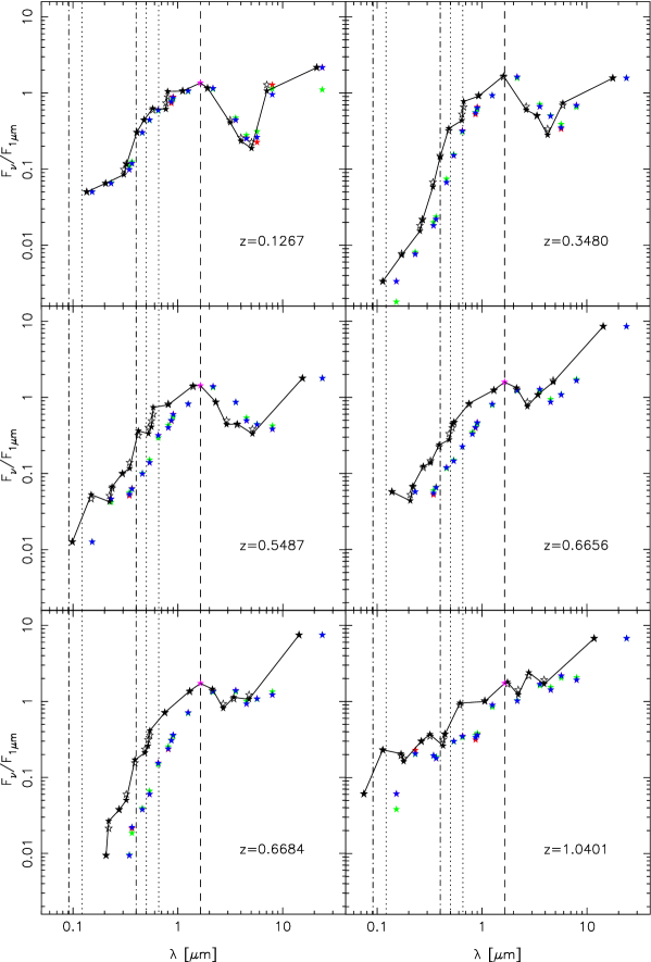
Figure 1.— Example templates obtained from the VVDS dataset (data normalized to the 1 $\mu$m  flux density). The original redshift of the source is given for each galaxy. Red stars show the original SED of the galaxy. Black open stars show the $z=0$ derived template without a K-correction calculation. Green stars show the recovered SED built by convolution of the $z=0$ non-K-corrected template with the filter response curves. Black filled stars (joined by a black line) show the final $z=0$ template after applying the K-correction. Blue stars show the final recovered redshifted template (which must coincide with the template formed by red stars). In each plot, the 1.6 $\mu$m  bump is marked with a dashed line (and a magenta filled star), the Lyman and 4000 Å  breaks are marked with dashed-dotted lines, and the positions of the Ly$\alpha$, $[OIII]\lambda\lambda 4959,5007$ and H$\alpha+[NII]\lambda\lambda 6548,6584$ emission-lines are marked with dotted lines.

We performed a visual inspection of all the templates, rejecting those with unusual shapes due to deviant photometry points. The final training sets were formed by 317 and 542 sources for the VVDS and HDFN datasets, respectively. To these, we also added the Devriendt et al. (1999) 17 empirically-calibrated templates. Some representative examples of our templates are shown in Figure 1. These examples show that the most prominent feature of the great majority of the SEDs is the 1.6 $\mu$m  stellar bump (marked with a dashed line). Nonetheless, for some galaxies this feature is hardly visible (see the bottom-right template in Figure 1). This absence of the stellar bump is observed in some of the most infrared-luminous (presumably AGN-dominated) galaxies in the local Universe (see, e.g., Sanders et al., 1988; Devriendt et al., 1999). Despite the low resolution of the SEDs, some other spectral features are also visible, such as emission-lines in the UV/optical (marked with dotted lines), the 4000 Å  break (dashed-dotted line), or emission from PAHs in the MIR.

After building the set of empirical templates, we redshifted them to values in the $0<z<3$ range using a step of $\Delta z=0.005$. The redshift range was chosen based on expectations prior to launch (Dole et al., 2003). These redshifted templates were then convolved with the filter responses.

The redshift estimation proceeded as follows. First, the entire observed SED was fitted with a Chebysev polynomial. When possible (i.e., when there were NIR and IRAC data and the stellar bump was present), the derivative of this polynomial was used to estimate the position of the 1.6 $\mu$m  bump and its uncertainty. This position was used as a first guess and to constrain the final solution (in the range formed by the bump value and its error). We found this step to be a good procedure to get rid of outliers. Second, the observed and template fluxes were normalized to one of the bands (the reference band mentioned in Section 2.4) to account for the effects of different luminosities. Data points with dubious photometric calibration or repeated observations (two observations for the same filter) were removed before the fitting. In addition, the data points at the edges of the SEDs (the bluest and reddest filters, the latter always being 24 $\mu$m), were given smaller weights in the fitting, or removed when the templates had no data at those wavelengths. Third, the templates and observed values were compared and a most probable redshift was calculated by minimizing a reduced $\chi^{2}$ estimator of the form:

$$\chi^{2}=\frac{1}{(N_{\mathrm{filt}}-1)}\sum_{1}^{N_{\mathrm{filt}}}\frac{(F^{i}_{\mathrm{template}}-F^{i}_{\mathrm{observed}})^{2}}{(\Delta F^{i}_{\mathrm{observed}})^{2}}$$ (A1)

where $N_{\mathrm{filt}}$ is the number of filters considered, $F_{\mathrm{template}}$ is the flux calculated for each redshifted template in the $ith$ filter, and $F_{\mathrm{observed}}$ and $\Delta F^{i}_{\mathrm{observed}}$ are the measured fluxes and uncertainties in each filter. Errors in the redshift were calculated with a $\Delta\chi^{2}$ algorithm, and were quoted as the $z$-range for which the solution has a 68% probability of being correct. We only obtained redshifts for galaxies with more than four points in the SED (virtually all the sources mentioned in Section 2.4).

A.3. Comparison with the spectroscopic sample

Comparison between the photometric redshifts obtained in this work and the spectroscopic redshifts measured in CDFS (left panel) and in HDFN (right panel). Both comparisons refer to the photometric redshift results obtained with the complete template set (built with 317 sources from VVDS, 542 from TKRS and Cowie et al. 2004, and the 17 templates in Devriendt et al. 1999). Gray symbols are sources with unreliable spectroscopic redshifts. Open stars are sources detected in less than five bands. The dashed line shows the equality line, and the dash-dotted ones show the $\sigma_{z}/(1+z)<0.1$ area.

The redshifts obtained with our photometric technique were compared with the spectroscopic values for all the galaxies in the sample. In Figure A.3, we demonstrate that our procedure is able to recover the redshifts of the galaxies used as an input for the technique.

The left panel in this Figure shows the comparison of photometric and spectroscopic redshifts for CDFS when using the complete template set (876 templates in total). The distribution of points is very symmetric around the equality line. The median value for the difference between the derived photometric redshift and the spectroscopic one ($\delta z$ hereafter) is $\delta z=0.003$, showing there is no systematic difference. Given that the wavelength scales in terms of $(1+z)$ when going to more distant sources, it seems more physically meaningful to discuss errors in terms of $\sigma_{z}/(1+z)$ (Wolf et al., 2004), where $\sigma_{z}$ is the absolute value of $\delta z$. For the VVDS comparison, 90% of the objects have values of $\sigma_{z}/(1+z)<0.2$, 82% of the objects have values of $\sigma_{z}/(1+z)<0.1$, and 75% have $\sigma_{z}/(1+z)<0.05$. The average (median) $\sigma_{z}/(1+z)$ is 0.050 (0.012). These statistics improve if we only take into account sources with highly reliable redshifts (as stated by VVDS): 98% of the objects have values of $\sigma_{z}/(1+z)<0.2$, 92% of the objects have values of $\sigma_{z}/(1+z)<0.1$, and 85% have $\sigma_{z}/(1+z)<0.05$.

The right panel of Figure A.3  shows the comparison of our photometric redshifts with spectroscopic redshifts in the HDFN when using the complete template set. The statistics for this comparison (for the highly-reliable spectroscopic sample) are very similar to the CDFS case: $<\delta z>=-0.003$, $<\sigma_{z}/(1+z)>=0.016$, 98% of the objects have values of $\sigma_{z}/(1+z)<0.2$, 97% of the objects have values of $\sigma_{z}/(1+z)<0.1$, and 95% have $\sigma_{z}/(1+z)<0.05$. It is interesting to notice the smaller scatter of the points around the equality line in comparison with what we found in CDFS. This difference is due to the larger number of sources having NIR data in the HDFN, which makes the photometric redshift estimation more reliable because the 1.6 $\mu$m  bump position can be better constrained.

The two panels in Figure A.3 show some outliers, a total of 75 objects with $\sigma_{z}/(1+z)>0.1$ for the left panel (18% of the total sample of 425 sources in CDFS), and 22 objects with $\sigma_{z}/(1+z)>0.1$ for the right panel (4% of the total sample of 601 sources in HDFN). We will discuss these photometric redshift failures next, in order to characterize why the photometric redshift technique fails. None of these outliers were included within the template set, either because of a unreliable spectroscopic redshift, or because they did not have more than ten points in their SEDs.

In CDFS, 60 out of the 75 outliers (i.e., 80% of the outliers) do not have highly-reliable spectroscopic redshifts (gray stars in Figure A.3). Out of these, 26 present slight differences with the spectroscopic redshifts of $\sigma_{z}/(1+z)<0.15$ (normally the redshift is overestimated). Out of the 34 remaining sources with unreliable spectroscopy, 18 present a clearly wrong photometric redshift. Half of these 18 sources present power-law like SEDs, and our method fails to obtain a good redshift. The other half do not present any particular problem, but the template selected by our technique gives a wrong redshift. The 16 remaining sources with non-reliable spectroscopy and $\sigma_{z}/(1+z)>0.15$ show SEDs clearly incompatible with the quoted spectroscopic redshifts. Out of the total 75 outliers in the left panel of Figure A.3, 15 are secured spectroscopic identifications, with 10 of them presenting $\sigma_{z}/(1+z)<0.15$. The other 5 do not have IRAC photometry, and our technique gives a very large redshift for them.

In HDFN, 4 out of the 22 outliers have less than 5 points in their SEDs. This kind of object was removed from the photometric redshift sample in this paper due to the high uncertainties related to the small number of data points. In fact, there are a total of 7 galaxies within this group with reliable spectroscopic redshift in the entire HDFN sample, which gives more than 50% (4 out of 7) having a wrong photometric redshift. There are 8 more outliers with unreliable spectroscopic redshifts. Out of these, 3 present slightly overestimated photometric redshifts, with differences with the spectroscopic redshifts of $\sigma_{z}/(1+z)<0.15$. Another 2 sources (out of the 8 with unreliable spectroscopy) present a clearly wrong photometric redshift (one of the gray stars at $z\sim 1.7$, and the gray star at $z_{\mathrm{photo}}=0$) due to highly deviant points in the SEDs (e.g., the $V$-band flux is 10 times larger than what would be expected based on other adjacent data points, the $BvR$ bands, in the $z_{\mathrm{photo}}\sim 1.7$ case). This deviant point could be linked to source variability or deblending problems. The 3 remaining sources with unreliable spectroscopy show SEDs clearly incompatible with the quoted spectroscopic redshifts. Out of the other 10 outliers found in the right panel of Figure A.3 (and having reliable spectroscopy), 4 of them present $\sigma_{z}/(1+z)<0.15$ (with a slightly overestimated photometric redshift). Another 6 are clearly wrong photometric redshifts, 3 of them lacking for NIR and/or IRAC data, and the other 3 objects presenting very disturbed SEDs.

In summary, the outliers in the two panels of Figure A.3 are sources with wrong photometric redshifts due to photometry problems (about one third of them), objects with slightly overestimated redshifts ($\sim$50% of them), or probably wrong spectroscopic redshifts (10%–20%). This demonstrates that the fitting method does not introduce significant errors in the redshift determination.

Left: Comparison between the photometric redshifts obtained in this work and the spectroscopic redshifts for HDFN sources. This comparison refers to the photometric redshift results obtained by using the templates built in CDFS (317 templates). Right: Comparison between the photometric redshifts obtained in this work and the spectroscopic redshifts for CDFS sources. This comparison refers to the photometric redshift results obtained by using the templates built in HDFN (542 templates). For both panels, gray symbols are sources with unreliable spectroscopic redshifts. Open stars are sources detected in less than five bands. The dashed line shows the equality line, and the dash-dotted ones show the $\sigma_{z}/(1+z)<0.1$ area.

Most of the galaxies plotted in the left panel (more precisely, 60%) and right panel (90%) of Figure A.3 were included in the template set used to derive photometric redshift. Therefore, the numbers given are not entirely representative of the goodness of the method presented in this paper. A real test of the method is presented in Figure A.3. Here we divided the sample in roughly two parts. One half of the sample was formed by the sources in CDFS, and the other half by sources in HDFN. We then obtained photometric redshifts for all the sources in one half of the sample by using the templates built from sources with a spectroscopic redshift within the other half of the sample. The left panel of Figure A.3 shows the comparison of photometric and spectroscopic redshifts for the HDFN sources when using the templates built from CDFS sources. The right panel in Figure A.3 shows the comparison for CDFS sources when only using templates from HDFN. The Figure demonstrates that we are able to obtain photometric redshifts (for the sources with secure spectroscopic redshift) with $\sigma_{z}/(1+z)<0.1$ for at least 80% of the sample (80% for the left panel and 84% for the right one), and redshifts with $\sigma_{z}/(1+z)<0.2$ for more than 90% of the galaxies (91% for the left panel and 94% for the right one). Other statistics are: $<\delta z>=-0.001$, $<\sigma_{z}/(1+z)>=0.078$ for the left panel and $<\delta z>=-0.002$, $<\sigma_{z}/(1+z)>=0.077$ for the right panel.

We also analyzed all the outliers on Figure A.3 to characterize why the photometric redshift technique fails. In the left panel, there are 601 galaxies with spectroscopic redshifts, 125 (21% of the total spectroscopic sample in HDFN) of which present $\sigma_{z}/(1+z)>0.1$. Out of this number, 67 sources (54% of the outliers) have $\sigma_{z}/(1+z)<0.2$, half of them with overestimated photometric redshifts, half with underestimated values. Within the 58 sources remaining (from the 125 outliers), 7 galaxies present very disturbed SEDs (6% of the outliers). Another 36 objects are clear photometric redshift errors (29% of the outliers), probably because of the lack of NIR and/or IRAC data (13 objects out of the 36), or because they present power-law SEDs (10 objects). The rest, 15 sources (12% of the outliers), are probable spectroscopic redshift errors (virtually all of them flagged as unreliable spectroscopic estimations). In the right panel of Figure A.3, there are 425 galaxies, 81 (19% of the total spectroscopic sample in CDFS) which present $\sigma_{z}/(1+z)>0.1$. Out of this number, 25 (31% of the outliers) have $\sigma_{z}/(1+z)>0.2$, and only 10 of those are labeled as secure spectroscopic redshifts, all with very disturbed SEDs. In summary, less than 20% of the galaxies present $\sigma_{z}/(1+z)>0.1$, at least one third of those present $\sigma_{z}/(1+z)>0.2$, and from these 10%, at least one fourth are probable spectroscopic redshift errors. Most of the sources with $\sigma_{z}/(1+z)>0.1$ either lack for NIR/IRAC photometry, or present disturbed SEDs probably linked to source variability (related to AGN activity) or deblending problems. In fact, $\sim$6% of the sources with $\sigma_{z}/(1+z)<0.1$ present multiple identifications (within the search radius), in comparison with a $\sim$10% for galaxies with $\sigma_{z}/(1+z)>0.1$.

Comparison between the photometric redshifts obtained in this work (using the complete template set) and the ones obtained by COMBO17 (Wolf et al., 2004) in CDFS. Gray symbols are sources with $\Delta z>0.05$ as given by COMBO17. Open stars are sources detected in less than five bands. The dashed line shows the equality line, and the dash-dotted ones show the $\sigma_{z}/(1+z)<0.1$ area.

Finally, we also compared our results with other photometric redshift surveys such as COMBO17 (Wolf et al., 2004). COMBO17 and our redshifts agree very well up to $z\sim 1$, with more than 90% of the sources being within the $\sigma_{z}/(1+z)<0.1$ area (just for a highly-reliable sample, i.e., sources with $\Delta z<0.05$ as given by COMBO17). However, there are two issues in the comparison, that we can clearly see in Figure A.3. First, the distribution of points is not symmetric at $z\gtrsim 1$. Many sources lying near the COMBO17 redshift limit ($z\sim 1.4$) are placed at higher redshifts by our photometric redshift method, most of them presenting high COMBO17 redshift uncertainties. For $0<z_{COMBO17}<1.4$, we find: $<\delta z>=0.052$, $<\sigma_{z}/(1+z)>=0.114$, and 75% of the sources have $\sigma_{z}/(1+z)<0.1$. COMBO17 is known to have a deficiency when estimating redshifts at $z\geq 1$, because the useful spectral features go out of their optical filter set. These are also the faintest sources in the COMBO17 sample, and the photometric redshift method gets more uncertain. In our case, NIR data are available for 50% of the sources, and IRAC photometry for virtually all of them. These bands allow us to trace the spectral features used by COMBO17 to high redshift ($z\sim 3$), and to break redshift degeneracies coming from the misidentification of the Balmer break with the Lyman break. The second issue seen in Figure A.3 is that some galaxies (approximately 5% of the common sources between our survey and COMBO17) are placed at $z<0.2$ by COMBO17 and at higher redshifts by our work. Le Floc’h et al. (2005) also noticed this effect in studying the luminosities of MIPS sources in CDFS, concluding that they must be redshift outliers in the COMBO17 survey.

The statistics and the fraction of outliers of our photometric redshift technique are comparable to most other photometric redshift works in the literature (e.g., Connolly et al. 1995; Chen et al. 2003; Firth et al. 2003; Rowan-Robinson 2003; Babbedge et al. 2004; Zheng et al. 2004), and only slightly worse than some surveys aimed at obtaining high-quality photometric redshift by using adequate sets of narrow-band filters, although the new Spitzer data helps to obtain more reliable and accurate redshifts for $z\gtrsim 1$ sources (e.g., Wolf et al. 2004).

Although Le Floc’h et al. (2004) demonstrated the ability of Spitzer  to identify sources in the ’redshift desert’ ($1.5<z<3.0$, Steidel et al., 2004), our photo-$z$ technique might have deficiencies for this redshift range. The spectroscopic surveys are highly biased towards $z<1$ galaxies, given their technical limitations for very faint objects. Indeed, our template set does not have many galaxies lying at high redshifts: 80% of the templates correspond to $z<1$ sources, 16% to $1.0<z<1.4$ galaxies, and only 4% above $z=1.4$. Our technique assumes that the most distant galaxies in our sample are very similar (in their SED properties) to the closer ones, i.e., we can find templates fitting the $z>1.4$ galaxies among the $z<1.4$ sample. Figure 4.2 shows that this extrapolation is not unreasonable, given that the LIRG population (probably showing similar properties at all redshifts) dominates our sample (in number of sources) from $z\sim 0.8$ up to $z\sim 2.0$. Only above $z\sim 2.0$, the ULIRGs are statistically relevant in number, and we do not have many templates with known spectroscopic redshifts.

Having this possible problem in mind, we performed a visual inspection of the fits for the galaxies identified as being at $z>1.4$ by our photo-$z$ technique. This test is represented in Figure A.3, which plots 10 sources selected randomly from the entire sample in the redshift range $0<z<1.4$ (left column), and 10 more at $1.4<z<3.0$ (right column). This figure gives an overview of the reliability of our photo-$z$ technique. Most of the galaxies in our sample show a clear 1.6 $\mu$m  stellar bump, a feature that allows a reliable photometric redshift determination. Indeed, all $z<1.4$ galaxies in Figure A.3 show a negative average slope in the IRAC bands, and a positive slope in the optical/NIR bands, pointing to a clear 1.6 $\mu$m  bump. The determination of the exact position of this bump is, however, importantly affected by the availability of NIR data (and consequently, the uncertainty in the photometric redshift). For the sources at $z>1.4$, at least 7 galaxies present a change in slope (from positive to negative) inside the spectral range covered by IRAC, which indicates the presence of the 1.6 $\mu$m  bump (for a $1.3\lesssim z\lesssim 4$ galaxy). The visual inspection of the randomly selected sources in Figure A.3 revealed that the assigned redshift was dubious for 20%–25% of the sources, all of them lacking a marked 1.6 $\mu$m  stellar bump (probably linked to the presence of an AGN), and preferentially lying at $z>1.4$. This percentage is very similar to the total reliability of our technique ($\sim 80$%), previously discussed in this Section, which suggests that the procedure remains applicable to the highest redshift range. A better coverage of the ’redshift desert’ for LIRGs and ULIRGs by spectroscopic surveys would be desirable to reduce the uncertainty of the results achieved at $z>1.4$.

Some randomly-selected examples of the fits obtained in the photometric redshift estimation. On the left, we show ten sources selected randomly in the redshift range $0<z<1.4$, and on the right ten more randomly selected sources at $1.4<z<3.0$ are given. Photometry points are plotted with stars, and the best template fit to the data is shown with a solid line.

Appendix B SYSTEMATIC UNCERTAINTIES IN THE LUMINOSITY FUNCTION ESTIMATION LINKED TO PHOTOMETRIC REDSHIFT ERRORS

In this Appendix, we will investigate the effect of the photometric redshift errors discussed in Appendix A (i.e., scatter and fraction of outliers) in the estimation of the luminosity functions.

The photometric redshift errors propagate in the calculation of luminosities. Given that the estimation of the luminosity functions involves binning and averaging of luminosities, the uncertainties linked to redshift errors could in principle diminish, and they should most probably be random. However, there could also exist some systematic uncertainties, specially in the extremes of the luminosity function (faint and bright ends), where the number of detected galaxies is small, and the redshift outliers are preferentially found.

To understand the uncertainties in the luminosity function linked to photometric redshift errors, we performed a Monte Carlo simulation similar to the one presented in Chen et al. (2003). This simulation consisted in the generation of an artificial catalog of galaxies following an assumed input Schechter luminosity function and presenting the characteristic limiting fluxes of our survey. Each galaxy was assigned a random redshift between $z=0$ and $z=3$. This redshift was perturbed by an amount linked to the probability distribution built from the scatter of points in the comparison between spectroscopic and photometric redshifts presented in Figure A.3. This probability distribution of photometric redshift uncertainties accounts for the scatter of points around the equality line in Figure A.3, and for the outliers (i.e., the most deviant points in that scattering plot, caused by photometry problems or any other issue). Finally, we estimated the luminosity function for three representative redshift intervals: $0.0<z<0.2$, $0.8<z<1.0$, and $1.8<z<2.2$. We will concentrate our discussion in the lowest redshift interval, $0.0<z<0.2$, where we can explore the largest luminosity range. Note that this interval only probes the photometric redshift errors toward higher redshifts. Given that we obtained very similar results for the other intervals, we concluded that the errors toward lower redshifts do not affect the results from our simulation significantly.

The results from the Monte Carlo simulation are plotted in Figure 2. The input luminosity function (continuous line) is not well recovered with the standard SWML method (open stars fitted by the dotted line). As we previously suggested, the photometric redshift errors affect the faint and bright ends of the luminosity function, resulting on an overestimation of the galaxy density in these ranges, which turns into an overestimation of both $\alpha$ (by $\sim$20%) and $L^{*}$ (by $\sim$0.3 dex). This result is consistent with that found by Chen et al. (2003). Note, however, that although the luminosity function parameters are not properly recovered due to photometric redshift errors, the integrated luminosity density does not change significantly (less than 0.1 dex, below the estimated uncertainty 0.25 dex).

Figure 2.— Results from the Monte Carlo simulation performed to investigate the systematic uncertainties in the 12 $\mu$m  luminosity function estimation introduced by the photometric redshift errors. The solid line shows the input Schechter luminosity function, whose $\alpha$ and $L^{*}$ values are indicated by the triangle in the inset. The open stars and dotted line (also in the inset, with the contour delimiting the 99.99% probability area) show the recovered luminosity function for the artificial catalog. These open stars have been offset to higher luminosities by a constant small amount for clarity. The filled stars and dash-dotted line (also in the inset) represent the final luminosity function obtained with the modified SWML method (using a Monte Carlo iterative method). This technique accounts for the typical luminosity function errors (linked to the number of galaxies in each luminosity bin), as well as for redshift uncertainties.

To cope with the previously described systematic errors, we modified the SWML luminosity function method to include the photometric redshift and luminosity uncertainties. We used a Monte Carlo approach where each redshift was treated as statistical variable with an average and an uncertainty. The average was the photometric redshift given by our technique and the uncertainty was derived from the probability distribution of redshift errors extracted from Figure A.3. The redshifts for the whole catalog of galaxies in our survey were randomly perturbed according to this distribution, and the 12 $\mu$m  luminosities and their uncertainties were recalculated. The luminosity function was estimated using the SWML method for the new catalog. We iterated this process 1000 times, and the final luminosity function points (given in Figures 4.3 and 4.3), the fitting parameters, and the associated errors for all these quantities were derived from the distribution of solutions.

The results from the modified SWML method for the simulation described previously are shown in Figure 2 with filled stars and a dash-dotted line (also in the inset). We are able to recover the input luminosity function parameters with high accuracy, reducing the systematic errors to less than 2% for $\alpha$, and less than 0.04 dex for both $L^{*}$ and $\phi^{*}$. In general, the modified SWML method obtained luminosity functions with smaller faint-end slopes and lower $L^{*}$ values than the traditional SWML technique for all the redshift ranges.

References

- Adelberger & Steidel (2000) Adelberger, K. L., & Steidel, C. C. 2000, ApJ, 544, 218
- Alonso-Herrero et al. (2004) Alonso-Herrero, A. et al. 2004, ApJS, 154, 155
- Alonso-Herrero et al. (2005) Alonso-Herrero et al. 2005, ApJ (submitted)
- Armus et al. (2004) Armus, L. et al. 2004, ApJS, 154, 178
- Arnouts et al. (2002) Arnouts, S., Vandame, B., Benoist, C., Groenewegen, M. A. T., da Costa, L., Schirmer, M., Mignani, R. P., & Slijkhuis, R. 2002, VizieR Online Data Catalog, 337, 90740
- Babbedge et al. (2004) Babbedge, T. S. R. et al. 2004, MNRAS, 353, 654
- Baldry et al. (2005) Baldry, I. K. et al. 2005, MNRAS, 165
- Barger et al. (2000) Barger, A. J., Cowie, L. L., & Richards, E. A. 2000, AJ, 119, 2092
- Bauer et al. (2005) Bauer, A. E., Drory, N., Hill, G. J., & Feulner, G. 2005, ApJ, 621, L89
- Bell & de Jong (2001) Bell, E. F., & de Jong, R. S. 2001, ApJ, 550, 212
- Bell et al. (2003) Bell, E. F., McIntosh, D. H., Katz, N., & Weinberg, M. D. 2003, ApJS, 149, 289
- Bell et al. (2005) Bell et al. 2005, ApJ (in press), astro-ph/0502246
- Benítez (2000) Benítez, N. 2000, ApJ, 536, 571
- Bertin & Arnouts (1996) Bertin, E., & Arnouts, S. 1996, A&AS, 117, 393
- Blain et al. (1999) Blain, A. W., Smail, I., Ivison, R. J., & Kneib, J.-P. 1999, MNRAS, 302, 632
- Bolzonella et al. (2000) Bolzonella, M., Miralles, J.-M., & Pelló, R. 2000, A&A, 363, 476
- Bouwens et al. (2004) Bouwens, R. J. et al. 2004, ApJ, 606, L25
- Brandt et al. (2001) Brandt, W. N. et al. 2001, AJ, 122, 1
- Brodwin et al. (2003) Brodwin et al. 2003, ApJ (submitted), astro-ph/0310038
- Bruzual & Charlot (2003) Bruzual, G., & Charlot, S. 2003, MNRAS, 344, 1000
- Budavári et al. (2005) Budavári, T. et al. 2005, ApJ, 619, L31
- Burgarella et al. (2005) Burgarella, D. et al. 2005, ApJ, 619, L63
- Calura & Matteucci (2003) Calura, F., & Matteucci, F. 2003, ApJ, 596, 734
- Capak et al. (2004) Capak, P. et al. 2004, AJ, 127, 180
- Cardiel et al. (2003) Cardiel, N., Elbaz, D., Schiavon, R. P., Willmer, C. N. A., Koo, D. C., Phillips, A. C., & Gallego, J. 2003, ApJ, 584, 76
- Chary et al. (2004) Chary, R. et al. 2004, ApJS, 154, 80
- Chary & Elbaz (2001) Chary, R., & Elbaz, D. 2001, ApJ, 556, 562
- Chen et al. (2003) Chen, H. et al. 2003, ApJ, 586, 745
- Cohen (2002) Cohen, J. G. 2002, ApJ, 567, 672
- Coleman et al. (1980) Coleman, G. D., Wu, C.-C., & Weedman, D. W. 1980, ApJS, 43, 393
- Colina & Bohlin (1994) Colina, L., & Bohlin, R. C. 1994, AJ, 108, 1931
- Collister & Lahav (2004) Collister, A. A., & Lahav, O. 2004, PASP, 116, 345
- Condon (1989) Condon, J. J. 1989, ApJ, 338, 13
- Condon et al. (2002) Condon, J. J., Cotton, W. D., & Broderick, J. J. 2002, AJ, 124, 675
- Connolly et al. (1995) Connolly, A. J., Csabai, I., Szalay, A. S., Koo, D. C., Kron, R. G., & Munn, J. A. 1995, AJ, 110, 2655
- Connolly et al. (1997) Connolly, A. J., Szalay, A. S., Dickinson, M., Subbarao, M. U., & Brunner, R. J. 1997, ApJ, 486, L11
- Corradi et al. (1996) Corradi, R. L. M., Beckman, J. E., & Simonneau, E. 1996, MNRAS, 282, 1005
- Cowie et al. (2004) Cowie, L. L., Barger, A. J., Hu, E. M., Capak, P., & Songaila, A. 2004, AJ, 127, 3137
- Cowie et al. (1999) Cowie, L. L., Songaila, A., & Barger, A. J. 1999, AJ, 118, 603
- Cowie et al. (1996) Cowie, L. L., Songaila, A., Hu, E. M., & Cohen, J. G. 1996, AJ, 112, 839
- Dale & Helou (2002) Dale, D. A., & Helou, G. 2002, ApJ, 576, 159
- Devriendt et al. (1999) Devriendt, J. E. G., Guiderdoni, B., & Sadat, R. 1999, A&A, 350, 381
- Dickinson et al. (2003) Dickinson, M., Papovich, C., Ferguson, H. C., & Budavári, T. 2003, ApJ, 587, 25
- Dole et al. (2003) Dole, H., Lagache, G., & Puget, J.-L. 2003, ApJ, 585, 617
- Drory et al. (2004) Drory, N., Bender, R., Feulner, G., Hopp, U., Maraston, C., Snigula, J., & Hill, G. J. 2004, ApJ, 608, 742
- Drory et al. (2001) Drory, N., Bender, R., Snigula, J., Feulner, G., Hopp, U., Maraston, C., Hill, G. J., & de Oliveira, C. M. 2001, ApJ, 562, L111
- Efstathiou et al. (1988) Efstathiou, G., Ellis, R. S., & Peterson, B. A. 1988, MNRAS, 232, 431
- Egami et al. (2004) Egami, E. et al. 2004, ApJS, 154, 130
- Elbaz et al. (2005) Elbaz et al. 2005, A&A(in press), astro-ph/0502569
- Förster Schreiber et al. (2003) Förster Schreiber, N. M., Genzel, R., Lutz, D., & Sternberg, A. 2003, ApJ, 599, 193
- Fadda et al. (2002) Fadda, D., Flores, H., Hasinger, G., Franceschini, A., Altieri, B., Cesarsky, C. J., Elbaz, D., & Ferrando, P. 2002, A&A, 383, 838
- Fang et al. (1998) Fang, F., Shupe, D. L., Xu, C., & Hacking, P. B. 1998, ApJ, 500, 693
- Fernández-Soto et al. (1999) Fernández-Soto, A., Lanzetta, K. M., & Yahil, A. 1999, ApJ, 513, 34
- Feulner et al. (2005) Feulner, G., Goranova, Y., Drory, N., Hopp, U., & Bender, R. 2005, MNRAS, 358, L1
- Firth et al. (2003) Firth, A. E., Lahav, O., & Somerville, R. S. 2003, MNRAS, 339, 1195
- Flores et al. (1999) Flores, H. et al. 1999, ApJ, 517, 148
- Fontana et al. (2004) Fontana, A. et al. 2004, A&A, 424, 23
- Franceschini et al. (2001) Franceschini, A., Aussel, H., Cesarsky, C. J., Elbaz, D., & Fadda, D. 2001, A&A, 378, 1
- Franceschini et al. (2003) Franceschini, A. et al. 2003, A&A, 403, 501
- Franceschini et al. (2002) Franceschini, A., Fadda, D., Cesarsky, C. J., Elbaz, D., Flores, H., & Granato, G. L. 2002, ApJ, 568, 470
- Gabasch et al. (2004a) Gabasch, A. et al. 2004a, A&A, 421, 41
- Gabasch et al. (2004b) —. 2004b, ApJ, 616, L83
- Gallego et al. (2002) Gallego, J., García-Dabó, C. E., Zamorano, J., Aragón-Salamanca, A., & Rego, M. 2002, ApJ, 570, L1
- Gallego et al. (1995) Gallego, J., Zamorano, J., Aragón-Salamanca, A., & Rego, M. 1995, ApJ, 455, L1
- Georgakakis et al. (2003) Georgakakis, A., Hopkins, A. M., Sullivan, M., Afonso, J., Georgantopoulos, I., Mobasher, B., & Cram, L. E. 2003, MNRAS, 345, 939
- Giavalisco et al. (2004a) Giavalisco, M. et al. 2004a, ApJ, 600, L103
- Giavalisco et al. (2004b) —. 2004b, ApJ, 600, L93
- Glazebrook et al. (2004) Glazebrook, K. et al. 2004, Nature, 430, 181
- Glazebrook et al. (2003) —. 2003, ApJ, 587, 55
- Glazebrook et al. (1999) Glazebrook, K., Blake, C., Economou, F., Lilly, S., & Colless, M. 1999, MNRAS, 306, 843
- Gordon et al. (1997) Gordon, K. D., Calzetti, D., & Witt, A. N. 1997, ApJ, 487, 625
- Gordon et al. (2005) Gordon et al. 2005, PASP (in press)
- Gwyn & Hartwick (1996) Gwyn, S. D. J., & Hartwick, F. D. A. 1996, ApJ, 468, L77
- Haarsma et al. (2000) Haarsma, D. B., Partridge, R. B., Windhorst, R. A., & Richards, E. A. 2000, ApJ, 544, 641
- Hammer et al. (1997) Hammer, F. et al. 1997, ApJ, 481, 49
- Heavens et al. (2004) Heavens, A., Panter, B., Jimenez, R., & Dunlop, J. 2004, Nature, 428, 625
- Hippelein et al. (2003) Hippelein, H. et al. 2003, A&A, 402, 65
- Hogg (2002) Hogg, D. 2002, ApJL, astro-ph/0105280
- Hogg et al. (1998) Hogg, D. W., Cohen, J. G., Blandford, R., & Pahre, M. A. 1998, ApJ, 504, 622
- Hopkins (2004) Hopkins, A. M. 2004, ApJ, 615, 209
- Hopkins et al. (2001) Hopkins, A. M., Connolly, A. J., Haarsma, D. B., & Cram, L. E. 2001, AJ, 122, 288
- Hopkins et al. (2000) Hopkins, A. M., Connolly, A. J., & Szalay, A. S. 2000, AJ, 120, 2843
- Hornschemeier et al. (2001) Hornschemeier, A. E. et al. 2001, ApJ, 554, 742
- Houck et al. (2005) Houck et al. 2005, A&A(in press), astro-ph/0502216
- Huang et al. (2004) Huang, J.-S. et al. 2004, ApJS, 154, 44
- Huchra & Sargent (1973) Huchra, J., & Sargent, W. L. W. 1973, ApJ, 186, 433
- Hughes et al. (1998) Hughes et al. 1998, Nature, 394, 241
- John (1988) John, T. L. 1988, A&A, 193, 189
- Juneau et al. (2005) Juneau, S. et al. 2005, ApJ, 619, L135
- Kauffmann et al. (2003) Kauffmann, G. et al. 2003, MNRAS, 341, 33
- Kennicutt (1998) Kennicutt, R. C. 1998, ARA&A, 36, 189
- Kron (1980) Kron, R. G. 1980, ApJS, 43, 305
- La Franca et al. (2004) La Franca, F. et al. 2004, AJ, 127, 3075
- Labbe et al. (2005) Labbe, I. et al. 2005, ApJ (in press), astro-ph/0504219
- Lacy et al. (2004) Lacy, M. et al. 2004, ApJS, 154, 166
- Lagache et al. (2004) Lagache, G. et al. 2004, ApJS, 154, 112
- Lanzetta et al. (2002) Lanzetta, K. M., Yahata, N., Pascarelle, S., Chen, H., & Fernández-Soto, A. 2002, ApJ, 570, 492
- Lanzetta et al. (1996) Lanzetta, K. M., Yahil, A., & Fernandez-Soto, A. 1996, Nature, 381, 759
- Lawrence et al. (1986) Lawrence, A., Walker, D., Rowan-Robinson, M., Leech, K. J., & Penston, M. V. 1986, MNRAS, 219, 687
- Le Fèvre et al. (2004) Le Fèvre, O. et al. 2004, A&A, 428, 1043
- Le Floc’h et al. (2004) Le Floc’h, E. et al. 2004, ApJS, 154, 170
- Le Floc’h et al. (2005) Le Floc’h et al. 2005, ApJ (submitted)
- Leitherer et al. (1999) Leitherer et al. 1999, ApJS, 123, 3
- Lilly et al. (1996) Lilly, S. J., Le Fevre, O., Hammer, F., & Crampton, D. 1996, ApJ, 460, L1
- Lilly et al. (1995) Lilly, S. J., Tresse, L., Hammer, F., Crampton, D., & Le Fevre, O. 1995, ApJ, 455, 108
- Machalski & Godlowski (2000) Machalski, J., & Godlowski, W. 2000, A&A, 360, 463
- Madau et al. (1996) Madau, P., Ferguson, H. C., Dickinson, M. E., Giavalisco, M., Steidel, C. C., & Fruchter, A. 1996, MNRAS, 283, 1388
- Madau et al. (1998) Madau, P., Pozzetti, L., & Dickinson, M. 1998, ApJ, 498, 106
- Marleau et al. (2004) Marleau, F. R. et al. 2004, ApJS, 154, 66
- Martin et al. (2005) Martin, D. C. et al. 2005, ApJ, 619, L59
- Marzke et al. (1999) Marzke, R. et al. 1999, in Astronomical Society of the Pacific Conference Series, 148
- Massarotti et al. (2001) Massarotti, M., Iovino, A., & Buzzoni, A. 2001, ApJ, 559, L105
- McCarthy et al. (2004) McCarthy, P. J. et al. 2004, ApJ, 614, L9
- McLeod et al. (1993) McLeod, K. K., Rieke, G. H., Rieke, M. J., & Kelly, D. M. 1993, ApJ, 412, 111
- Mo et al. (1998) Mo, H. J., Mao, S., & White, S. D. M. 1998, MNRAS, 295, 319
- Moorwood et al. (2000) Moorwood, A. F. M., van der Werf, P. P., Cuby, J. G., & Oliva, E. 2000, A&A, 362, 9
- Pérez-González et al. (2003a) Pérez-González, P. G., Gil de Paz, A., Zamorano, J., Gallego, J., Alonso-Herrero, A., & Aragón-Salamanca, A. 2003a, MNRAS, 338, 508
- Pérez-González et al. (2003b) —. 2003b, MNRAS, 338, 525
- Pérez-González et al. (2003c) Pérez-González, P. G., Zamorano, J., Gallego, J., Aragón-Salamanca, A., & Gil de Paz, A. 2003c, ApJ, 591, 827
- Papovich & Bell (2002) Papovich, C., & Bell, E. F. 2002, ApJ, 579, L1
- Papovich et al. (2001) Papovich, C., Dickinson, M., & Ferguson, H. C. 2001, ApJ, 559, 620
- Papovich et al. (2004) Papovich, C. et al. 2004, ApJS, 154, 70
- Papovich et al. (2005) Papovich et al. 2005, ApJ (submitted)
- Pettini et al. (1998) Pettini, M., Kellogg, M., Steidel, C. C., Dickinson, M., Adelberger, K. L., & Giavalisco, M. 1998, ApJ, 508, 539
- Poli et al. (2003) Poli, F. et al. 2003, ApJ, 593, L1
- Pozzi et al. (2004) Pozzi, F. et al. 2004, ApJ, 609, 122
- Rieke et al. (1993) Rieke, G. H., Loken, K., Rieke, M. J., & Tamblyn, P. 1993, ApJ, 412, 99
- Rieke & Low (1972) Rieke, G. H., & Low, F. J. 1972, ApJ, 176, L95
- Rigby et al. (2004) Rigby, J. R. et al. 2004, ApJS, 154, 160
- Rigopoulou et al. (2002) Rigopoulou, D., Franceschini, A., Aussel, H., Genzel, R., Thatte, N., & Cesarsky, C. J. 2002, ApJ, 580, 789
- Rowan-Robinson (2003) Rowan-Robinson, M. 2003, MNRAS, 345, 819
- Rush et al. (1993) Rush, B., Malkan, M. A., & Spinoglio, L. 1993, ApJS, 89, 1
- Sadler et al. (2002) Sadler, E. M. et al. 2002, MNRAS, 329, 227
- Sajina et al. (2005) Sajina, A., Lacy, M., & Scott, D. 2005, ApJ, 621, 256
- Sanders & Mirabel (1996) Sanders, D. B., & Mirabel, I. F. 1996, ARA&A, 34, 749
- Sanders et al. (1988) Sanders, D. B., Soifer, B. T., Elias, J. H., Neugebauer, G., & Matthews, K. 1988, ApJ, 328, L35
- Saunders et al. (1990) Saunders, W., Rowan-Robinson, M., Lawrence, A., Efstathiou, G., Kaiser, N., Ellis, R. S., & Frenk, C. S. 1990, MNRAS, 242, 318
- Sawicki (2002) Sawicki, M. 2002, AJ, 124, 3050
- Sawicki et al. (1997) Sawicki, M. J., Lin, H., & Yee, H. K. C. 1997, AJ, 113, 1
- Schechter (1976) Schechter, P. 1976, ApJ, 203, 297
- Schiminovich et al. (2005) Schiminovich, D. et al. 2005, ApJ, 619, L47
- Schmidt (1968) Schmidt, M. 1968, ApJ, 151, 393
- Serjeant et al. (2001) Serjeant, S. et al. 2001, MNRAS, 322, 262
- Serjeant et al. (2002) Serjeant, S., Gruppioni, C., & Oliver, S. 2002, MNRAS, 330, 621
- Somerville et al. (2001) Somerville, R. S., Primack, J. R., & Faber, S. M. 2001, MNRAS, 320, 504
- Spinoglio & Malkan (1989) Spinoglio, L., & Malkan, M. A. 1989, ApJ, 342, 83
- Spinoglio et al. (1995) Spinoglio, L., Malkan, M. A., Rush, B., Carrasco, L., & Recillas-Cruz, E. 1995, ApJ, 453, 616
- Steidel et al. (1999) Steidel, C. C., Adelberger, K. L., Giavalisco, M., Dickinson, M., & Pettini, M. 1999, ApJ, 519, 1
- Steidel et al. (2004) Steidel, C. C., Shapley, A. E., Pettini, M., Adelberger, K. L., Erb, D. K., Reddy, N. A., & Hunt, M. P. 2004, ApJ, 604, 534
- Sullivan et al. (2001) Sullivan, M., Mobasher, B., Chan, B., Cram, L., Ellis, R., Treyer, M., & Hopkins, A. 2001, ApJ, 558, 72
- Sullivan et al. (2000) Sullivan, M., Treyer, M. A., Ellis, R. S., Bridges, T. J., Milliard, B., & Donas, J. . 2000, MNRAS, 312, 442
- Tacconi et al. (2002) Tacconi, L. J., Genzel, R., Lutz, D., Rigopoulou, D., Baker, A. J., Iserlohe, C., & Tecza, M. 2002, ApJ, 580, 73
- Takagi et al. (2003) Takagi, T., Vansevicius, V., & Arimoto, N. 2003, PASJ, 55, 385
- Takeuchi et al. (2003) Takeuchi, T. T., Yoshikawa, K., & Ishii, T. T. 2003, ApJ, 587, L89
- Teplitz et al. (2003) Teplitz, H. I., Collins, N. R., Gardner, J. P., Hill, R. S., & Rhodes, J. 2003, ApJ, 589, 704
- Tresse & Maddox (1998) Tresse, L., & Maddox, S. J. 1998, ApJ, 495, 691
- Tresse et al. (2002) Tresse, L., Maddox, S. J., Le Fèvre, O., & Cuby, J.-G. 2002, MNRAS, 337, 369
- Treyer et al. (1998) Treyer, M. A., Ellis, R. S., Milliard, B., Donas, J., & Bridges, T. J. 1998, MNRAS, 300, 303
- Vandame et al. (2001) Vandame, B. et al. 2001, ArXiv Astrophysics e-prints
- Willmer (1997) Willmer, C. N. A. 1997, AJ, 114, 898
- Wilson et al. (2002) Wilson, G., Cowie, L. L., Barger, A. J., & Burke, D. J. 2002, AJ, 124, 1258
- Wilson et al. (2004) Wilson, G. et al. 2004, ApJS, 154, 107
- Wirth et al. (2004) Wirth, G. D. et al. 2004, AJ, 127, 3121
- Wolf et al. (2004) Wolf, C. et al. 2004, A&A, 421, 913
- Wyder et al. (2005) Wyder, T. K. et al. 2005, ApJ, 619, L15
- Xu et al. (1998) Xu, C. et al. 1998, ApJ, 508, 576
- Xu et al. (2003) Xu, C. K., Lonsdale, C. J., Shupe, D. L., Franceschini, A., Martin, C., & Schiminovich, D. 2003, ApJ, 587, 90
- Yan et al. (1999) Yan, L., McCarthy, P. J., Freudling, W., Teplitz, H. I., Malumuth, E. M., Weymann, R. J., & Malkan, M. A. 1999, ApJ, 519, L47
- Zheng et al. (2004) Zheng, W. et al. 2004, ApJS, 155, 73