Abstract

The present work shows that a combination of nonlinear contributions from the Ricci curvature in Einstein field equations can drive a late time acceleration of expansion of the universe. The transit from the decelerated to the accelerated phase of expansion takes place smoothly without having to resort to a study of asymptotic behaviour. This result emphasizes the need for thorough and critical examination of models with nonlinear contribution from the curvature.

1 INTRODUCTION

The search for a dark energy component, the driver of the present accelerated expansion of the universe, has gathered a huge momentum because the alleged acceleration is now believed to be a certainty, courtesy the WMAP data [1]. As no single candidate enjoys a pronounced supremacy over the others as the dark energy component in terms of its being able to explain all the observational details as well as having a sound field theoretic support, any likely candidate deserves a careful scrutiny until a final unambiguous solution for the problem emerges. The cosmological constant $\Lambda$, a minimally coupled scalar field with a potential, Chaplygin gas or even a nonminimally coupled scalar field are amongst the most popular candidates ( see ref. [2] for a comprehensive review). Recently an attempt along a slightly different direction is gaining more and more importance. This effort explores the possibility whether geometry in its own right could serve the purpose of explaining the present accelerated expansion. The idea actually stems from the fact that higher order modifications of the Ricci curvature $R$, in the form of $R^{2}$ or $R_{\mu\nu}R^{\mu\nu}$ etc. in the Einstein - Hilbert action could generate an accelerated expansion in the very early universe [3]. As the curvature $R$ is expected to fall off with the evolution, it is an obvious question if inverse powers of $R$ in the action, which should become dominant during the later stages, could drive a late time acceleration.

A substantial amount of work in this direction is already there in the literature. Capozziello et al. [4] introduced an action where $R$ is replaced by $R^{n}$ and showed that it leads to an accelerated expansion, i.e, a negative value for the deceleration parameter $q$ for $n=-1$ and $n=\frac{3}{2}$. Carroll et al. [5] used a combination of $R$ and $\frac{1}{R}$, and a conformally transformed version of theory, where the effect of the nonlinear contribution of the curvature is formally taken care of by a scalar field, could indeed generate a negative value for the deceleration parameter. Vollick also used this $1/R$ term in the action [6] and the resulting field equations allowed an asymptotically exponential and hence accelerated expansion. The dynamical behaviour of $R^{n}$ gravity had been studied in detail by Carloni et.al [7]. A remarkable result obtained by Nojiri and Odinstov [8] shows that it may indeed be possible to attain an inflation at an early stage and also a late surge of accelerated expansion from the same set of field equations if the modified Lagrangian has the form $\it{L}=R+R^{m}+R^{-n}$ where $m$ and $n$ are positive integers. However, the solutions obtained are piecewise, i.e, large and small values of the scalar curvature $R$, corresponding to early and late time behaviour of the model respectively, are treated separately. But this clearly hints towards a possibility that different modes of expansion at various stages of evolution could be accounted for by a curvature driven dynamics. Other interesting investigations such as that with an inverse $sinh(R)$ [9] or with $lnR$ terms [10] in the action are also there in the literature.

The question of stability [11] and other problems notwithstanding, these investigations surely open up an interesting possibility for the search of dark energy in the non-linear contributions of the scalar curvature in the field equations. However, in most of these investigations so far mentioned, the present acceleration comes either as an asymptotic solution of the field equations in the large cosmic time limit, or even as a permanent feature of the dynamics of the universe. But both the theoretical demand [12] as well as observations [13] ( see also ref [1] ) clearly indicate that the universe entered into its accelerated phase of expansion only very recently and had been decelerating for the major part of its evolution. So the deceleration parameter $q$ must have a signature flip from a positive to a negative value only in a recent past.

In the present work, we write down the field equations for a general Lagrangian $f(R)$ and investigate the behaviour of the model for two specific choices of $f(R)$, namely $f(R)=R-\frac{\mu^{4}}{R}$ and $f(R)=e^{-\frac{R}{6}}$.

Although the field equations, a set of fourth order differential equations for the scale factor $a$, could not be completely solved analytically, the evolution of the ‘acceleration’ of the universe could indeed be studied at one go, i.e, without having to resort to a piecewise solution. The results obtained are encouraging, both the examples show smooth transitions from the decelerated to the accelerated phase. In this work we virtually assume nothing regarding the relative strengths of different terms and let them compete in their own way, and still obtain the desired transition in the signature of the deceleration parameter $q$. This definitely provides a very strong support for the host of investigations on curvature driven acceleration, particularly those quoted in references [5, 6 and 7].

In the evolution equation, $q$ is expressed as a function of $H$, the Hubble parameter. This enables one to write an equation with only $q$ to solve for; as the only other variable remains is $H$ which becomes the argument. This method appears to be extremely useful, although it finds hardly any application in the literature. The only example noted by us is the one by Carroll et al. [14], which, however, describes the nature only in an asymptotic limit.

In the next section the model with two examples are described and in the last section we include some discussion.

2 Curvature driven acceleration

The relevant action is

$$\it A=\int[\frac{1}{16\pi G}f(R)+L_{m}]\sqrt{-g}d^{4}x,$$ (1)

where the usual Einstein - Hilbert action is generalized by replacing $R$ with $f(R)$, which is an analytic function of $R$, and $L_{m}$ is the Lagrangian for all the matter fields. A variation of this action with respect to the metric yields the field equations as

$$G_{\mu\nu}=R_{\mu\nu}-\frac{1}{2}Rg_{\mu\nu}={T_{\mu\nu}}^{c}+{T_{\mu\nu}}^{M},$$ (2)

where the choice of units $8\pi G=1$ has been made. ${T_{\mu\nu}}^{M}$ represents the contribution from matter fields scaled by a factor of $\frac{1}{f^{\prime}(R)}$ and ${T_{\mu\nu}}^{c}$ denotes that from the curvature to the effective stress energy tensor. ${T_{\mu\nu}}^{c}$ is actually given as

$${T_{\mu\nu}}^{c}=\frac{1}{f^{\prime}(R)}[\frac{1}{2}g_{\mu\nu}{(f(R)-Rf^{\prime}(R))}+{f^{\prime}(R)}^{;\alpha\beta}(g_{\mu\alpha}g_{\nu\beta}-g_{\mu\nu}g_{\alpha\beta})].$$ (3)

A prime indicates differentiation with respect to Ricci scalar $R$. It deserves mention that we use a variation of (1) w.r.t. the metric tensor as in Einstein - Hilbert variational principle and not a Palatini variation where $A$ is varied w.r.t. both the metric and the affine connections. As the actual focus of the work is to scrutinize the role of geometry alone in driving an acceleration in the later stages, we shall work without any matter content, i.e, $L_{m}=0$ leading to ${T_{\mu\nu}}^{M}=0$. So for a spatially flat Robertson - Walker spacetime, where

$$ds^{2}=dt^{2}-a^{2}(t)[dr^{2}+r^{2}d\theta^{2}+r^{2}sin^{2}\theta d\phi^{2}],$$ (4)

the field equations (2) take the form ( see ref. [4] )

$$3\frac{\dot{a}^{2}}{a^{2}}=\frac{1}{f^{\prime}}[{\frac{1}{2}(f-Rf^{\prime})-3\frac{\dot{a}}{a}\dot{R}f^{\prime\prime}}],~{}~{}~{}~{}~{}~{}~{}~{}~{}~{}~{}~{}~{}~{}~{}~{}$$ (5)

$$2\frac{\ddot{a}}{a}+\frac{\dot{a}^{2}}{a^{2}}=-\frac{1}{f^{\prime}}[{2\frac{\dot{a}}{a}\dot{R}f^{\prime\prime}+\ddot{R}f^{\prime\prime}+\dot{R}^{2}f^{\prime\prime\prime}-\frac{1}{2}(f-Rf^{\prime})}].$$ (6)

Here $a$ is the scale factor and an overhead dot indicates differentiation w.r.t. the cosmic time $t$. If $f(R)=R$, the equation (2) and hence (5) and (6) take the usual form of vacuum Einstein field equations. It should be noted that the Ricci scalar $R$ is given by

$$R=-6[\frac{\ddot{a}}{a}+\frac{\dot{a}^{2}}{a^{2}}],$$ (7)

and already involves a second order time derivative of $a$. As equation (6) contains $\ddot{R}$, one actually has a system of fourth order differential equations.

It deserves mention at this stage that if $R$ is a constant, then whatever form of $f(R)$ is chosen except $f(R)=R$, equations (5) and (6) represent a vacuum universe with a cosmological constant and hence yield a deSitter solution, i.e, an ever accelerating universe. Evidently we are not interseted in that, we are rather in search of a model which clearly shows a transition from a decelerated to an accelerated phase of expansion of the universe. As we are looking for a curvature driven acceleration at late time, and the curvature is expected to fall off with the evolution, we shall take a form of $f(R)$ which has a sector growing with the fall of $R$. We work out two examples where indeed the primary purpose is served.

(i) $f(R)=R-\frac{\mu^{4}}{R}.$

In the first example, we take

$$f(R)=R-\frac{\mu^{4}}{R},$$ (8)

where $\mu$ is a constant. Indeed $\mu$ has a dimension, that of $R^{\frac{1}{2}}$, i.e, that of $(time)^{-1}$. This is exactly the form used by Carroll et al. [5] and Vollick [6]. Using the expression (8) in a combination of the field equations (5) and (6), one can easily arrive at the equation

$$2\dot{H}=\frac{1}{(R^{2}+\mu^{4})}[{2\mu^{4}\frac{\ddot{R}}{R}-6\mu^{4}\frac{\dot{R}^{2}}{R^{2}}-2\mu^{4}H\frac{\dot{R}}{R}}],$$ (9)

where $H=\frac{\dot{a}}{a}$, is the Hubble parameter. As both $R$ and $H$ are functions of $a$ and its derivatives, equation (9) looks set for yielding the solution for the scale factor. But it involves fourth order derivatives of $a$ ( $R$ already contains $\ddot{a}$ ) and is highly nonlinear. This makes it difficult to obtain a completely analytic solution for $a$. As opposed to the earlier investigations where either a piecewise or an asymptotic solution was studied, we adopt the following strategy. The point of interest is the evolution of the deceleration parameter

$$q=-\frac{a\ddot{a}}{\dot{a}^{2}}=-\frac{\dot{H}}{H^{2}}-1.$$ (10)

So we translate equation (9) into the evolution equation for $q$ using equation (10) and obtain

$~{}~{}~{}~{}~{}~{}~{}~{}~{}~{}~{}~{}~{}~{}\mu^{4}\frac{\ddot{q}}{(q-1)}-3\mu^{4}\frac{\dot{q}^{2}}{(q-1)^{2}}+\mu^{4}H^{2}(q+1)(4q+7)-3\mu^{4}q(q+1)H^{2}\frac{(2q-3)}{(q-1)}$

$$-10\mu^{4}H^{2}(q+1)^{2}+36H^{6}(q-1)^{2}(q+1)=0.$$ (11)

This equation, although still highly nonlinear, is a second order equation in $q$. But the problem is that both $q$ and $H$ are functions of time and cannot be solved for with the help of a single equation. However, they are not independent and are connected by equation (10). So we replace time derivatives by derivatives w.r.t. $H$ using equation (10) and write (11) as

$$\frac{1}{3}(q^{2}-1)H^{2}q^{\dagger\dagger}+{[\frac{1}{3}(q-1)+(q+1)]}H^{2}{q^{\dagger}}^{2}+\frac{2}{3}H(q^{2}-1)q^{\dagger}+H^{4}(q-1)^{4}-(q-1)(4q^{2}-4q-1)=0.$$ (12)

Here for the sake of simplicity $\mu^{4}$ is chosen to be 12 ( in proper units ), and a dagger represents a differentiation w.r.t. the Hubble parameter $H$. As $\frac{1}{H}$ is a measure of the age of the universe and $H$ is a monotonically decreasing function of the cosmic time, equation (12) can now be used as the evolution equation for $q$. The equation appears to be hopelessly nonlinear to give an analytic solution but if one provides two initial conditions, for $q$ and $q^{\dagger}$, for some value of $H$, a numerical solution is definitely on cards. We choose units so that $H_{0}$, the present value of $H$, is unity and pick up sets of values for $q$ and $q^{\dagger}$ for $H=1$ ( i.e, the present values ) from observationally consistent region [15] and plot $q$ versus $H$ numerically. As the inverse of $H$ is the estimate for the cosmic age, ‘future’ is given by $H<1$ and past by $H>1$. The plots speak for themselves. One has the desired feature of a negative $q$ at $H=1$ and it comes to this negative phase only in the recent past. Furthermore, in near future, $q$ has another sign flip in the opposite direction, forcing an exhibition of a decelerated expansion in the future again. An important point to note here is that neither the nature of the plots, nor the values of $H$ at which the transitions take place, crucially depend on the choice of initial conditions, so the model is reasonably stable. It is interesting to note the asymptotic values of $q$. For very high values of the cosmic time, i.e, for $H\rightarrow 0$ , $q\rightarrow 1$ or $q\rightarrow(\frac{1\pm\sqrt{2}}{2})$. So it admits at least one negative value, consistent with the results obtained in ref. [5]. As $f(R)$ contains $R^{n}$ with $n\leq 1$, one does not expect this to give rise to an early inflation. For $H\rightarrow\infty$, i.e, for $t\rightarrow 0$, $q\rightarrow+1$, which exhibits indeed a non-inflationary decelerating model.

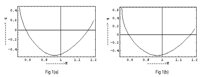
Figure 1: Figure 1(a) and 1(b) shows the plot of $q$ vs. $H$ for $f(R)=R-\frac{\mu^{4}}{R}$ for different initial conditions. For figure 1(a) we choose the initial conditions as $q[1]=-0.5$, $q^{\prime}[1]=1.2$ whereas for figure 1(b) we set the initial conditions as $q[1]=-0.5$, $q^{\prime}[1]=1.0$.

(ii) $f(R)=e^{-\frac{R}{6}}$ .

In this choice, the function $f$ is monotonically increasing with $t$ as $R$ is decreasing with $t$. The field equations (5) and (6) have the form

$$3\frac{\dot{a}^{2}}{a^{2}}=-6[{\frac{1}{2}(1+\frac{R}{6})-\frac{1}{12}\frac{\dot{a}}{a}\dot{R}}],~{}~{}~{}~{}~{}~{}~{}~{}~{}~{}~{}~{}~{}~{}~{}~{}$$ (13)

$$2\frac{\ddot{a}}{a}+\frac{\dot{a}^{2}}{a^{2}}=-6[{\frac{1}{2}(1+\frac{R}{6})-\frac{1}{18}\frac{\dot{a}}{a}\dot{R}-\frac{1}{36}\ddot{R}+\frac{1}{216}\dot{R}^{2}}].$$ (14)

From these two equations it is easy to write

$$2\dot{H}=\frac{1}{6}\ddot{R}-\frac{1}{36}\dot{R}^{2}-\frac{1}{6}H\dot{R}.$$ (15)

Following the same method as before, the evolution of $q$ as a function of $H$ can be written as

$H^{4}(q+1)q^{\dagger\dagger}+{[H^{4}-(q+1)H^{6}}]{q^{\dagger}}^{2}+[2(q+1)H^{3}+6qH^{3}+3H^{3}-4H^{5}(q^{2}-1)]q^{\dagger}$

$$+6H^{2}q^{2}+2H^{2}q-4H^{4}(q^{2}-1)(q-1)-8H^{2}+2=0.$$ (16)

With similar initial conditions for $q$ and $q^{\dagger}$ at $H=1$, the plot of $q$ versus $H$ ( figure 2 ) shows features very similar to the previous example, the deceleration parameter $q$ has two signature changes, from a positive to a negative phase in the recent past ( $H>1$ ) and in the reverse direction in the near future ( $H<1$ ). In this case also, a small change in initial conditions hardly has any perceptible change in the graphs.

As for the asymptotic behaviour, one expects that as exponential functions have higher powers, the model could lead to an early inflation. Actually it does; for $H\rightarrow\infty$, i.e, for small $t$, $q\rightarrow-1$. The equation (16) does not straightaway lead to the other extreme end, $H\rightarrow 0$, i.e, $t\rightarrow$ large. Actually a common factor of $(q+1)$ had been cancelled while arriving at equation (16). So $q=-1$ is the other solution, which holds for $H\rightarrow 0$ limit. So here also, the model has a steady acceleration at the far future end.

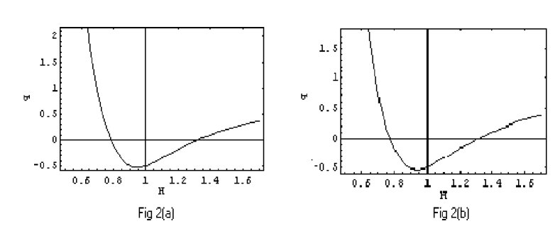
Figure 2: Figure 2(a) and 2(b) shows the plot of $q$ vs. $H$ for $f(R)=e^{-\frac{R}{6}}$ for different initial conditions. Here also for figure 2(a) and 2(b) we set the initial conditions as $q[1]=-0.5$, $q^{\prime}[1]=1.0$ and $q[1]=-0.5$, $q^{\prime}[1]=1.2$ respectively.

As the plots provide a sufficient data set, attempts could be made to find the closest analytical expression for $q=q(H)$. These expressions are found to be polynomials. For example, a very close analytical expression for figure 2(b), within the accuracy of plots, is given as

$$q=47.95H^{6}-335.73H^{5}+991H^{4}-1586.90H^{3}+1459.20H^{2}-729.73H+153.74.$$ (17)

This expression holds only when $H$ is reasonably close to one, and has nothing to do with other ranges of values of $H$.

3 Discussion

The present work indicates that by asking the question whether geometry in its own right can lead to the late surge of accelerated expansion, some feats can surely be achieved. Both the examples considered here indicate that one can build up models which starts accelerating at the later stage of evolution and thus allow all the past glories of the decelerated model like nucleosynthesis or structure formation to remain intact. An added bonus of the examples is that in both the cases the universe re-enters a decelerated phase in near future and the ‘phantom menace’ is avoided - the universe does not have to have a singularity of infinite volume and infinite rate of expansion in a ‘finite’ future.

It is of course true that a lot of other criteria has to be satisfied before one makes a final choice, and we are nowhere near that. Already there is a criticism of $\frac{1}{R}$ gravity that it is unsuitable for local astrophysics because of problems regarding stability [11]. However, it was pointed out by Nojiri and Odinstov [8] that a polynomial may save the situation ( see also reference [16] ). Our second example is exponential in $R$, i.e, a series of positive powers in $R$, and hence could well satisfy the criterion of stability. As already pointed out, although the choice of $f(R)=R-\frac{\mu^{4}}{R}$ is already there in the literature and served the purpose in a restricted sense than it does in the present work, the choice of $f(R)=e^{-\frac{R}{6}}$ has hardly any mention in the literature.

It should also be noted that the present toy model deals with a vacuum universe and one has to either put in matter, or derive the relevant matter at the right epoch from the curvature itself. Some efforts towards this have already begun [17]. On the whole, there are reasons to be optimistic about a curvature driven acceleration which might become more and more important in view of the fact that WMAP data could indicate a very strong constraint on the variation of the equation of state parameter $w$ [18].

4 Acknowledgement

Authors are thankful to Mriganka Chakraborty for useful discussion.

References

-
[1]
D. N. Spergel et al., Astrophys. J. Suppl., 148, 175 (2003);
L. Page, astro-ph/0302220;
L. Verde et al., Astrophys. J. Suppl., 148, 195 (2003);
S. Bridle, O. Lahav, J. P. Ostriker and P. J. Steinhardt, Science, 299, 1532 (2003);
C. Bennet et al., astro-ph/0302207;
G. Hinshaw et al., astro-ph/0302217;
A. Kognt et al., astro-ph/0302213. -
[2]
V. Sahni, astro-ph/0403324;
T. Padmanabhan, Phys. Rep., 380, 235 (2003). -
[3]
A. A. Starobinsky, Phys. Lett. B, 91, 99 (1980);
R. Kerner, Gen. Rel. Gravit., 14, 453 (1982);
J. P. Duruisseau, R. Kerner, Class. Quant. Grav., 3, 817 (1986). -
[4]
S. Capozziello, S. Carloni, A. Troisi, astro-ph/0303041;
S. Capozziello, V. F. Cardone, S. Carloni, A. Troisi, astro-ph/0307018. - [5] S. M. Carroll, V. Duvvuri, M. Trodden, M. S. Turner, astro-ph/0306438.
- [6] D. N. Vollick, Phys. Rev. D, 68, 063510 (2003).
- [7] S. Carloni, P.K.S. Dunsby, S. Capozziello and A. Troisi, gr-qc/0410046.
- [8] S. Nojiri and S. D. Odinstov, Phys. Rev. D, 68, 123512 (2003).
- [9] A. Borowiec and M. Francaviglia, hep-th/0403264.
- [10] S. Nojiri and S. D. Odinstov, hep-th/0308176.
- [11] A. D. Dolgov and M. Kawasaki, astro-ph/0307285.
-
[12]
T. Padmanabhan and T. Roychoudhury, astro-ph/0212573;
T. Roychoudhury and T. Padmanabhan, Astron. Astrophys, 429, 807 (2005). - [13] A. G. Riess, astro-ph/0104455.
- [14] S. M. Carroll et al., astro-ph/0410031.
-
[15]
U. Alam, V. Sahni, T. D. Saini and A. A. Starobinsky,
Mon. Not. Roy. Ast. Soc., 344, 1057 (2003); [ astro-ph/0303009];
U. Alam and V. Sahni, astro-ph/0209443. -
[16]
J. D. Barrow and A. C. Ottewill, J. Phys. A, 16,
2756 (1983);
S. Nojiri and S. D. Odinstov, Mod. Phys. Lett. A, 19, 627 (2004). -
[17]
M. Abdalla, S. Nojiri and S. D. Odinstov, Class. Quant.
Grav., 22, L35 (2005);
G. Allemandi, A. Borowiec, M. Francaviglia and S. D. Odinstov, gr-qc/0504057. - [18] H. K. Jassal, J. S. Bagla and T. Padmanabhan, Mon. Not. R. Astron. Soc., 356, L11 (2005).