Modeling the formation of galaxy clusters in MOND

Abstract

We use a one dimensional hydrodynamical code to study the evolution of spherically symmetric perturbations in the framework of Modified Newtonian Dynamics (MOND). The code evolves spherical gaseous shells in an expanding Universe by employing a MOND-type relationship between the fluctuations in the density field and the gravitational force, $g$. We focus on the evolution of initial density perturbations of the form $\delta_{i}\sim r_{i}^{-s}$ for $0<s<3$. A shell is initially cold and remains so until it encounters the shock formed by the earlier collapse of shells nearer to the centre. During the early epochs $g$ is sufficiently large and shells move according to Newtonian gravity. As the physical size of the perturbation increases with time, $g$ gets smaller and the evolution eventually becomes MOND dominated. However, the density in the inner collapsed regions is large enough that they re-enter the Newtonian regime. The evolved gas temperature and density profiles tend to a universal form that is independent of the the slope, $s$, and of the initial amplitude. An analytic explanation of this intriguing result is offered. Over a wide range of scales, the temperature, density and entropy profiles in the simulations, depend on radius roughly like $r^{0.5}$, $r^{-1.5}$ and $r^{1.5}$, respectively. We compare our results with XMM-Newton and Chandra observations of clusters. The temperature profiles of 16 observed clusters are either flat or show a mild decrease at $R\lower 2.15277pt\hbox{$\;\buildrel>\over{\sim}\;$}200\rm kpc$. MOND profiles show a significant increase that cannot reconciled with the data. Our simulated MOND clusters are substantially denser than the observed clusters. It remains to be seen whether these difficulties persist in three-dimensional hydrodynamical simulations with generic initial conditions.

1 introduction

In the standard cosmological paradigm the Universe is predominantly filled with dark matter (DM). The success of this paradigm is indisputable. It explains a multitude of observational data over a wide range of scales, from rotation curves of local galaxies to the anisotropies of the cosmic microwave background (CMB) at high redshifts.

Despite this success, several fundamental problems remain to be resolved. Although the best evidence for DM is the flattening of rotation curves of many spiral galaxies, the scenario does not explain the shape of these curves in the inner regions of some galaxies (e.g de Blok et al. 2001, Hayashi et al. 2004). The DM scenario predicts specific correlations between the internal properties of clusters of galaxies (e.g. the mass vs temperature, entropy vs temperature). While such correlations are observed, their parameters do not agree with the model predictions. There are various puzzles related to the evolution of the galaxy population as well. All these problems and several others can probably be attributed to physical processes unrelated to the dark matter. But they do allow us some leeway in exploring other alternatives to the DM scenario. One possibility is to superimpose additional forces acting only in the dark sector (e.g. Gradwohl & Frieman J.A. 1992; Farrar & Peebles 2004; Sealfon et al. 2005; Shirata et al. 2005). These forces can work in the direction of boosting the clustering on small scales, leaving the larger scales intact. Several desirable features follow from this scenario (e.g. Nusser, Gubser & Peebles 2005).

Another approach is to modify Newton’s $g_{{}_{N}}\sim 1/({\rm distance})^{2}$ law for the force of gravity, relinquishing the DM scenario altogether. This approach was originally introduced to account for the flattening of rotation curves without invoking dark matter (Milgrom 1983; Bekenstein & Milgrom 1984). After all, the DM particle has yet to be discovered (Bertone et al.  2004) and we lack an experimental verification of Newton’s laws at low accelerations. The essence of Modified Newtonian Dynamics (MOND) is to replace Newton’s law of gravity at sufficiently low accelerations $g_{{}_{N}}<g_{{}_{0}}$ by $g\sim\sqrt{g_{{}_{0}}g_{{}_{N}}}$ where $g_{{}_{0}}\approx 1.2\times 10^{-8}{\mathrm{c}m\;s^{-2}}$ is found to give the best results in fitting the rotation curves.

Recently a few attempts have been made to confront MOND with observations of the large scale structure (LSS) in the Universe (McGaugh 1999, Sanders 2001, Nusser 2002, Knebe & Gibson 2004, McGaugh 2004). When MOND is applied to a uniform background it predicts the collapse of any finite region in the Universe regardless of the mean density in that region (e.g., Felten 1984, Sanders 1998). To solve this problem Sanders (2001) proposed a two-field Lagrangian based theory of MOND in which the Friedmann-Robertson-Walker (FRW) background cosmology remains intact in the absence of fluctuations. He argued that this theory leads to LSS resembling Newtonian dynamics with CDM-like initial conditions. More recently Bekenstein (2004) proposed a general relativistic version of MOND in which the behaviour of cosmological background is very close to a FRW. Nusser (2002) employed the “Jeans swindle” (Binney & Tremain 1987) to write a MOND type relation between the fluctuations in the density and the gravitational force field. The relation can be derived from a Lagrangian and is equivalent to Sanders’ two-field theory in the limit of small coupling (Sanders 1998). And it seems that a similar relation can be derived from Bekenstein’s (2004) theory as well. Nusser (2002) then implemented this relation in a collisionless N-body code to simulate the evolution of LSS under MOND. This work showed that MOND, albeit with $g_{0}$ smaller than the standard value inferred from rotation curves, produces LSS similar to that seen in simulations of viable variants of the Cold Dark Matter (CDM) scenario. Knebe & Gibson (2004) used high resolution simulations of collisioness particles to study the LSS and “halo” profiles in MOND. According to these authors, MOND leads to reasonable predictions for the LSS even for the standard value of $g_{0}$. Knebe & Gibson also examined the properties of halos and concluded that density profiles in MOND have similar shape to the profiles seen in Newtonian simulations.

A MONDian Universe is dominated by ordinary baryonic matter made mainly of primordial hydrogen and helium. Baryons in cosmological systems have a relatively short mean free path, and should be treated as a hydrodynamical fluid. This fluid can collapse under its self-gravity, shock-heat during the collapse, cool, and form stars. Reliable three dimensional simulations of these processes are difficult and very CPU demanding, even in Newtonian dynamics where the Poisson equation can be solved efficiently. The problem is greatly simplified if one restricts the analysis to symmetric perturbations. Stachniewicz & Kutschera (2004) adopted this approach to the collapse of low mass objects at high redshifts using a spherically symmetric hydrodynamical code with MONDian gravity. In this paper we address the formation of clusters of galaxies in MOND using hydrodynamical simulations of spherically symmetric perturbations having initial power law profiles. The perturbations are evolved using a one dimensional Lagrangian hydrodynamical code. Cooling and heat conduction are not included in this code. These processes are important in galaxies and small groups of galaxies. However, they are likely to play a minor role in governing the evolution of the gaseous intercluster medium (ICM) in the outer regions of massive clusters. Several works have confronted MOND with observations of clusters (e.g. The & White 1988; Aguirre et al. 2001). Aguirre et al. (2001) assumed the hydrostatic equilibrium to derive MOND temperature profiles from X-ray data of three nearby clusters. They concluded that MOND predictions for the temperature profiles disagree with observations. Our approach here is to derive cluster properties resulting from the dynamical evolution of initial perturbations. This approach will enable us to make detailed predictions independently of the observations, and to test several key assumptions such as that of the hydrostatic equilibrium. Therefore, we expect it to provide stringent constraints on MOND from the observational data.

The remainder of the paper is organised as follows. The notation, the equations of motion, and the initial conditions are described in §2. An analytic treatment of the evolution when the perturbations are small is given in §2.2. The numerical model is outlined in §3. In §4, tests using known self-similar solutions are presented. The results for MOND are described §5. In §6 our results are confronted with recent observations. A final summary and discussion are presented in §7.

2 The modified cosmological equations of motion

The background FRW cosmology is described by the scale factor $a(t)$ normalised to unity at the present, the Hubble function $H(t)=\dot{a}/a$, and the total mean background matter density $\bar{\rho}_{tot}=\bar{\rho}_{\rm dm}+\rho_{\rm b}$, where $\bar{\rho}_{\rm dm}$ and $\rho_{\rm b}$ are the mean densities of the dark and baryonic matter, respectively. In MOND the Universe is made of baryonic matter and so we take ${\bar{\rho}}_{\rm dm}=0$. Further, we assume a vanishing cosmological constant since otherwise the cosmic age would be unrealistically long if $\rho_{\rm b}$ is fixed by nucleosynthesis. We also define $\Omega_{\rm b}=\bar{\rho}_{b}/\rho_{c}$, where $\rho_{c}=3H^{2}/(8\pi G)$ is the critical density. These cosmological quantities are related by Einstein equations of general relativity. Let ${\bf r}$ and ${\bf x}={\bf r}/a$ denote, respectively, physical and comoving coordinates. The fluctuations over the uniform background in the matter distribution are described by the comoving peculiar velocity ${\bf v}=\,{\rm d}{\bf x}/\,{\rm d}t$ of a patch of matter, the density contrast $\delta({\bf x})=\rho({\bf x})/\bar{\rho}-1$, where $\rho({\bf x})$ is the local density, and the fluctuations in the gravitational force field, ${\bf g}$. Further, the thermal state of the gas is described by the pressure, $P$ and the internal energy, $u$, which are assumed to be related to the density by a perfect equation of state $P=(\gamma-1)\rho u$, where $\gamma=5/3$. Here, we find it convenient to work with $p=P/{\bar{\rho}}$, instead of the physical pressure $P$. The Newtonian equations of motion governing the evolution of a spherical perturbation are: the continuity equation

$$\frac{\partial\delta}{\partial t}+\frac{1}{x^{2}}\partial_{x}[x^{2}(1+\delta)v]=0\;,$$ (1)

the Euler equation of motion,

$$\frac{\,{\rm d}v}{\,{\rm d}t}+2Hv=\frac{1}{a}g-\frac{1}{a^{2}}\frac{\partial_{x}p}{1+\delta}\;,$$ (2)

the energy equation,

$$\frac{\,{\rm d}u}{\,{\rm d}t}=\frac{p}{(1+\delta)^{2}}\frac{\,{\rm d}\delta}{\,{\rm d}t}-3Hu\;.$$ (3)

where the “pressure”, $P$, and internal energy, $u$, are related by the equation of state,

$$P=(\gamma-1)(1+\delta)u\;.$$ (4)

The final equation of motion that is needed is a relation between $g$ and the density, $\delta$. In the Newtonian theory $g=g_{{}_{\rm N}}$ where $g_{{}_{\rm N}}$ satisfies the Poisson equation,

$$\frac{1}{x^{2}}\partial_{x}(x^{2}g_{{}_{\rm N}})=-4\pi Ga\bar{\rho}_{\rm b}\delta=-\frac{3}{2}a\Omega_{\rm b}H^{2}\delta\;.$$ (5)

In MOND $g=g_{{}_{\rm M}}$ where $g_{{}_{\rm M}}$ is related to $g_{{}_{\rm N}}$ by $g_{{}_{\rm N}}=g_{{}_{\rm M}}\mu(g_{{}_{\rm M}}/g_{0})$ with $\mu(y)=y(1+y^{2})^{1/2}$ (Milgrom 1983, Bekenstein 2004). This relation yields

$$g_{{}_{\rm M}}=g_{{}_{\rm N}}\sqrt{\frac{1}{2}+\frac{1}{2}\sqrt{1+\left(\frac{2g_{0}}{g_{{}_{\rm N}}}\right)^{2}}}\;.$$ (6)

Neglecting thermal effects, the linear Newtonian theory implies that $|g|\gg g_{0}$ at sufficiently early times (see §2.2). But $|g|$ decreases with time and MOND eventually takes over the evolution of the perturbation. Matching MOND to observations of rotation curves of galaxies gives $g_{0}\simeq 1\times 10^{-10}\rm m\;s^{-2}$. We further assume that $g_{0}$ is constant with time.

2.1 Initial conditions

We chose a power law for the initial density contrast profile. We express the mean density contrast inside a distance $x$ from the centre of symmetry as

$$\bar{\delta}_{1}(z=0)=\delta_{0}\left(\frac{x}{x_{0}}\right)^{-s}$$ (7)

when normalised to redshift zero ($z=0$) according to Newtonian theory. We choose $\delta_{0}=1.68$ so that $x_{0}$ is roughly the Lagrangian size of the collapsed object at $z=0$. This physical meaning for $x_{0}$ is only valid in Newtonian dynamics. This way of normalising the perturbation has no bearing on the final results for MOND and is adopted here only for convenience.

The initial conditions are given at some very high redshift, $z_{1}$ as

$$\bar{\delta}_{1}(z_{1})=\frac{1}{D}\bar{\delta}_{1}(z=0)\;,$$ (8)

where $D$ is the (Newtonian) linear growth factor from $z_{1}$ until $z=0$ (e.g. Peebles 1980). The initial velocities are set according to the growing mode of linear theory as

$$v_{1}(x)=-\frac{\bar{\delta}_{1}(x)}{3}H_{1}x\;,$$ (9)

where $H_{1}=H(z_{1})$. The internal energy is

$$u_{1}(x)=0\;.$$ (10)

2.2 The limit of small density perturbations

Here we treat the limit of small density perturbation when $\delta\ll 1$ such that the convective terms in the equations of motion can be ignored. We will show that in this limit the density contrast tends to the form $\delta\propto 1/x$ independently of the amplitude and slope of the initial contrast density $\delta_{1}\propto x^{-s}$. We make the following assumptions. ($i)$ $\Omega_{\rm b}=1$ as is the case if the analysis is restricted to sufficiently early times, ($ii)$ the gas is initially cold and remains cold as long as $\delta\ll 1$ , and ($iii)$ the transition to the MOND regime is abrupt so that $g=g_{{}_{\rm N}}\sqrt{g_{n}/|g_{{}_{\rm N}}|}$ for $g\leq g_{0}$, and $g=g_{{}_{\rm N}}$ otherwise.

The initial mean density contrast, $\bar{\delta}_{1}=\delta_{0}(x/x_{0})^{-s}$, is given at some very high redshift $z_{1}$. We first assume that $s>1$. In this case $|g|\propto x\bar{\delta}_{1}\sim x^{1-s}$ decreases with radius, so that at redshift $z_{0}$, there exists a distance $x_{{}_{\rm M}}(z)$ such that all shells with $x\geq x_{{}_{\rm M}}(z_{0})$ are in the MOND regime, while those with $x<x_{{}_{\rm M}}(z_{0})$ are still in the Newtonian regime. We compute below the density profile for $x\gg x_{{}_{\rm M}}$. The reason for excluding shells at $x\lower 2.15277pt\hbox{$\;\buildrel>\over{\sim}\;$}x_{{}_{\rm M}}$ will become clear as we proceed. We assume that a shell at $x\gg x_{{}_{\rm M}}$ enters the MOND regime at $z_{{}_{\rm M}}(x)<z_{1}$. For $z_{1}>z>z_{{}_{\rm M}}$ all shells interior to $x$ are in the Newtonian regime and the amplitude of the peculiar gravitation force field at $x$ is given by

$$|g|=(1+z)^{2}\frac{\bar{\delta}(z){G\bar{M}}}{x^{2}}\;,$$ (11)

where $\bar{\delta}(z)$ is the density contrast at $z$, and ${\bar{M}}=(4\pi/3){\bar{\rho}}x^{3}$, $\bar{\rho}$ being the background density at redshift zero. In the Newtonian regime, we write $\bar{\delta}(z)=(1+z_{1})\bar{\delta}_{1}/(1+z)$. Therefore,

$$|g|=\frac{4\pi}{3}G\bar{\rho}\bar{\delta}_{1}(1+z_{1})(1+z)x\;.$$ (12)

The transition to the MOND regime occurs at $z_{{}_{\rm M}}$ at which $|g|=g_{0}$. Therefore,

$$\frac{1}{1+z_{{}_{\rm M}}}=\frac{4\pi}{3}(1+z_{1})\bar{\delta}_{1}G\bar{\rho}\frac{x}{g_{0}}\;.$$ (13)

The density contrast in the MOND regime grows like $1/(1+z)^{2}$ for sufficiently late times ($z\ll z_{{}_{\rm M}}$) (Nusser 2002). We can use this result if $x\gg x_{{}_{\rm M}}(z_{0})$ since this condition implies that $z_{0}\ll z_{{}_{\rm M}}$. The density at $z_{{}_{\rm M}}$ is $(1+z_{1})\bar{\delta}_{1}/(1+z_{{}_{\rm M}})$, which must be multiplied by $(1+z_{M})^{2}/(1+z_{0})^{2}$ to obtain the density, $\bar{\delta}(z_{0})$, at $z_{0}$. In this last step we have assumed that the mass of matter encompassed within a sphere of radius $x_{{}_{\rm M}}$, which is Newtonian, does not contribute significantly to $\bar{\delta}$ at $x\gg x_{{}_{\rm M}}$. The result is

$$\bar{\delta}(x,z_{0})=\frac{3g_{0}}{4\pi G\bar{\rho}}\frac{1}{(1+z_{0})^{2}}\frac{1}{x}\;,$$ (14)

for $x\gg x_{{}_{\rm M}}$ and $s>1$. For $s<1$ one can show that the last expression applies at $x\ll x_{{}_{\rm M}}$.

3 Numerical model

The evolution of a spherical perturbation in an otherwise uniform Universe is followed using a one-dimensional Lagrangian hydrodynamical code. The code follows the evolution of of $N$ shells inside a region of initial comoving radius $x_{\rm max}$. At the initial time, the shell $i+1/2$ is bounded by the $x_{i}=(i-1)\,{\rm d}x$ and $x_{i+1}=x_{i}+\,{\rm d}x$ where $\,{\rm d}x=x_{\rm max}/N$. The shell is then assigned a “mass”,

$$\,{\rm d}{\cal M}_{i+1/2}=\frac{4\pi}{3}\left[x_{i+1}^{3}(1+\bar{\delta}_{1}(x_{i+1}))-x_{i}^{3}(1+\bar{\delta}_{1}(x_{i}))\right]\;,$$ (15)

where $\bar{\delta}_{1}$ is given by (8). This mass is maintained constant throughout the evolution of the shell. The initial velocities at $x=x_{i}$ are set according to (9). A leapfrog integration scheme is used and so the positions, $x_{i}^{n}$, at the time step $t=t^{n}$ and the velocities, $v^{n+1/2}$, at $t=t^{n-1/2}=t^{n}-\,{\rm d}t^{n-1/2}/2$, are advanced as follows,

$$v^{n+1/2}_{i} = v^{n-1/2}_{i}\frac{1-H^{n}\,{\rm d}t^{n}}{1+H^{n}\,{\rm d}t^{n}}$$ (16)

$$-\left[\frac{4\pi(x_{i}^{n})^{2}}{(a^{n})^{2}}\frac{{\tilde{p}}_{i+1/2}^{n}-{\tilde{p}}_{i-1/2}^{n}}{\,{\rm d}{{\cal M}}_{i}}-\frac{g^{n}}{a^{n}}\right]\,{\rm d}t^{n}\;,$$

$$x_{i}^{n+1}=x_{i}^{n}+v_{i}^{n+1/2}\,{\rm d}t^{n+1/2}\;,$$ (17)

where

$$\,{\rm d}t^{n}=\frac{1}{2}(\,{\rm d}t^{n+1/2}+\,{\rm d}t^{n-1/2})\;,$$ (18)

$$\,{\rm d}{\cal M}_{i}=\frac{1}{2}(\,{\rm d}{\cal M}_{i-1/2}+\,{\rm d}{\cal M}_{i+1/2})\;,$$ (19)

and $\tilde{p}=p+q$, where $q$ accounts for artificial viscosity. Casting the standard expression for $q$ (e.g. Richtmyer & Morton 1967, Thoul & Weinberg 1995) in terms of comoving coordinates gives,

$$q^{n+1}_{i+1/2} = -\frac{2c_{q}(H^{n+1/2})^{2}}{(1+\delta^{n+1}_{i+1/2})^{-1}+(1+\delta^{n}_{i+1/2})^{-1}}$$ (21)

$$|V^{n+1/2}_{i+1}-V^{n+1/2}_{i}|(V^{n+1/2}_{i+1}-V^{n+1/2}_{i})\;,$$

if $V^{n+1/2}_{i+1}-V^{n+1/2}_{i}<0$, and $q^{n+1}_{i+1/2}=0$ otherwise. Here

$$V^{n+1/2}_{i}=\frac{a^{n+1/2}}{2}(x^{n+1}_{i+1}+x^{n}_{i})+\frac{a^{n+1/2}}{H^{n+1/2}}v^{n+1/2}_{i}$$ (22)

is equal to the actual total physical velocity and we take $c_{q}=4$ which would spread the shock over $\sim 4$ shells. In the Newtonian case the gravitational force field is

$$g^{n}_{i}=\frac{3(H^{n})^{2}}{8\pi}a^{n}\Omega^{n}\frac{\sum_{j}\,{\rm d}{\cal M}_{j+1/2}-\frac{4\pi}{3}x_{i}^{3}}{x_{i}^{2}}\;,$$ (23)

where the summation is over all $j$ having $x_{j}<x_{i}$. This expression is used in (6) to obtain the gravitational force field in MOND.

The density and energy are updated, respectively, according to

$$1+\delta^{n+1}_{i+1/2}=\frac{3\,{\rm d}{\cal M}_{i+1/2}}{4\pi\left[(x_{i+1}^{n+1})^{3}-(x_{i}^{n+1})^{3}\right]}\;,$$ (24)

and

$$u^{n+1}_{i+1/2} = u^{n}_{i+1/2}\frac{2-3H^{n+1/2}\,{\rm d}t^{n+1/2}}{2+3H^{n+1/2}\,{\rm d}t^{n+1/2}}$$ (25)

$$-\left[\frac{(p^{n+1}+p^{n})}{2}+q^{n}_{i+1/2}\right]$$

$$\times\left(\frac{1}{1+\delta^{n+1}_{i+1/2}}-\frac{1}{1+\delta^{n}_{i+1/2}}\right)\;.$$

The time-step $\,{\rm d}t^{n+1/2}$ is chosen to be the minimum of

$$c_{d}\sqrt{\frac{ax_{i}}{g_{i}}}\;,$$ (26)

$$c_{C}\frac{x_{i}-x_{i-1}}{\sqrt{\gamma(\gamma-1)u_{i}}}\;,$$ (27)

and

$$c_{v}\left|\frac{x_{i}-x_{i-1}}{v_{i}-v_{i-1}}\right|,$$ (28)

where we take $c_{d}=0.001$, $c_{C}=0.2$ and $c_{v}=0.05$ (Thoul & Weinberg 1995).

The boundary conditions are: $v_{i=1}=0$, and a $p_{{}_{N+1/2}}=0$. We have not included any explicit force softening in the code. For the number of shells we considered here the runs in all cases were completed within a few days of CPU time on a G4 machine.

4 Tests of the numerical scheme in the Newtonian case

Since the change from Newtonian gravity to MOND is trivial (see Eq. 6), it suffices to confront the code with self-similar solutions in the Newtonian case. For an adiabatic gas, the initial conditions given in Eq. (8–9) lead to self-similar evolution only in a flat Universe with $\Omega_{\rm b}=1$. Therefore, in this section we adopt this value of $\Omega_{\rm b}$. Here show results from the simulation output at redshift, $z=0.1$. Instead of scales variables (e.g. temperature and distance relative to their respective virial values) we work with physical quantities. The temperatures are given in degrees Kelvin, number densities in $\rm cm^{-3}$ and distances in $\rm kpc$. The advantage of using physical quantities is that they provide a more direct comparison with MOND where the mean density within the virial radius is not necessarily proportional to the background density.

We have run the code with $x_{0}=10\;\rm Mpc$ for three values of $s$: $s=0.25$, 2 and 2.8. We use $N=500$ shells for the runs with $s=0.25$ and $s=2$, and $N=100$ shells for $s=2.8$. The reason for the smaller number of shells for $s=2.8$ is that the code is substantially slower in this case as the time steps become extremely short at the later stages of the evolution. All simulations were run with an adiabatic index of $\gamma=5/3$.

In Newtonian dynamics, given the initial conditions Eq. (8-10), the evolution of a shell can be described qualitatively as follows. In the early stages the shell expands until it reaches its turnaround radius at which the total physical velocity, $aHx+av$, is zero. The shell then collapses towards the centre until it encounters the shock, transforming most of its kinetic energy into heat and become part of the hot region.

In Fig. 1 we plot the temperature (top panel) and density (bottom) versus the physical distance, $R$, from the output of the simulations at redshift $z=0.1$. The shock position, $R_{\rm sh}$, in the various cases corresponds to the abrupt change in the density and temperature. The transition in the shock is smoother for $s=2.8$ (dashed curve) as a result of the smaller number of shells in this run. The density variation across the shock for $s=0.25$ and $s=2$ is close to $(\gamma+1)/(\gamma-1)=4$, as expected in strong shocks. Because of the smaller number in the $s=2.8$ case, the density jump at the shock is weaker in this case.

At each time, $t$, there is a shell that is currently at its turnaround radius. This radius is (in physical units),

$$R_{\rm ta}=x_{0}(1+z)^{-(1+1/s)}\left(\frac{5}{3}\delta_{0}\right)^{1/s}\left(\frac{4}{3\pi}\right)^{(2/3)(1+1/s)}\;.$$ (29)

We have inspected the output of the simulations at various times and confirm that the turaround radii agree very well with (29). For $s=0.25$ and $s=2$, Chuzhoy & Nusser (2000) (hereafter CN2000) provided full self-similar solutions (see their figure 2). The shapes of our profiles match extremely well the solutions of CN2000. We also checked if the shock radius relative to the turnaround radius agrees with the self-similar solutions. At redshift $z=0.1$ we find, from (29), that $R_{\rm ta}=6.155\;\rm Mpc$ and $21.9~{}\rm Mpc$ for $s=2$ and $0.25$, respectively. Inferring the shock radii, $R_{\rm sh}$, from Fig. 1 we get $R_{\rm sh}/R_{\rm ta}\approx 1.8/6.155=0.29$ for $s=2$ and $0.57/21.9=0.026$ for $s=0.25$. These ratios agree very well with those inferred from figure 2 of CN2000.

For $s=2.8$ and $s=2$, the asymptotic logarithmic slopes near the origin agree very well with the analytic slopes presented in Table 1 of CN2000. For $s=0.25$, neither our curves nor those in figure 2 of CN2000 behave according to the asymptotic exponents in that Table. This is because the analytic exponents in the $s=0.25$ case are realized at extremely small fractions of the shock radius (see CN2000).

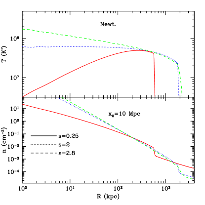
Figure 1: The temperature (top) and density (bottom) profiles at redshift $z=0$, obtained from the code for a power law initial profiles (see Eq.8) for $x_{0}=10\;\rm Mpc$. The various curves correspond to different values of the power law index, $s$, as indicated in the figure. The runs are for flat Universe with $\Omega_{b}=1$ and no dark matter. All curves agree well with the self-similar solutions of Chuzhoy & Nusser (2000).

5 Results with MOND

All results here will be presented for $g_{0}=1\times 10^{-10}\rm m\;s^{-2}$ and $\Omega_{\rm b}=0.044$. This value of $\Omega_{\rm b}$ is consistent with the observations of the deuterium abundance relative to hydrogen in Ly$\alpha$ clouds at high redshift (Kirkman et al. 2000). It is also consistent with the ratio of the first to second peak heights in the angular power spectrum of the CMB anisotropies (e.g. Spergel et al. 2003). We further take $h=0.7$ for the present Hubble constant (in units of $100\;\rm km\;s^{-1}Mpc^{-1}$). We work with a vanishing cosmological constant since otherwise the age of the Universe will be unreasonable large. For the cosmological parameters of choice, the age of the Universe $\approx 14\rm Gyr$.

The initial redshifts in all the runs is chosen sufficiently high so that all shells in the simulations are still Newtonian. We investigated various values for the parameters $s$ and $x_{0}$ (see Eq. 8). In Fig. 2 and Fig. 3 we show the temperature and the local baryon number density (in $\rm cm^{-3}$) versus the physical distance from the centre, $R$, for three different values of $s$, but the same $x_{0}$. The normalisation of the initial density profile is such that the average density contrast within a comoving distance $x_{0}$ is the same for all three values of $s$. There is a striking similarity in the shapes of the temperature and density profiles, respectively. This is in agreement with the analytic considerations in section § 2.2. The profiles are also insensitive to $x_{0}$ as seen in Fig. 3 which shows results for $s=1$ but different $x_{0}$. Even a change of a factor of 30 in $x_{0}$ fails to amount to any significant variation in the shape. The overall amplitude of both the temperature and the density profiles is also insensitive to $x_{0}$. The density and the temperature show, respectively, $\sim R^{-1.5}$ and $\sim R^{0.5}$, dependence on radius.

The “entropy”, $S=kT/n^{2/3}$, is plotted in Fig. 4. The entropy profiles corresponding to all the simulation outputs presented in the previous two figures are shown. In the shock heated regions the curves are practically indistinguishable at radii $R\lower 2.15277pt\hbox{$\;\buildrel>\over{\sim}\;$}200\rm kpc$. At these radii, $S\propto r^{1.5}$.

The redshift evolution for the case $s=1$ and $x_{0}=1\;\rm Mpc$ is explored in Fig. 5 showing profiles at three different redshifts. There is an increase by a factor of about 1.8 in the shock location between $z=0.5$ and $z=0.1$, but the profiles at these two redshifts have similar shapes. Over the distance scales in the plot the temperature shows a significant change from $z=3$ until the present. But the overall shape at $z=3$ is similar to the outer portion of the low redshift profiles. This indicates that the shape is preserved with redshift. The density profiles inside the shocked region at the three redshifts are remarkably similar, indicating that the system is in hydrostatic equilibrium.

At early epochs near the initial times, perturbations evolves according to Newtonian dynamics and then, as $|g|$ decreases, they succumb to MOND. This is as long as the perturbations are small. Fig. 6 demonstrates that in collapsed regions the perturbations become Newtonian again. The figure shows $|g|$ relative to $g_{0}$ as a function of $R$. In all cases $|g/g_{0}|>1$ in the inner regions.

The insensitivity of the profiles to the initial conditions is consistent with our findings in §2.2. A perturbation enters the MOND regime when the density fluctuations are still small. During this stage of the evolution they acquire the form (14) independently of the initial density profile, as shown in §2.2. Later evolution, when the density fluctuations are large, modified the form given in §2.2, but can not restore the dependence on the initial conditions. It is interesting that the evolved form of the density profile in MOND is $\sim r^{1.5}$ which is the same as the one obtained in the self-similar collapse of an initial $1/x$ perturbation in Newtonian dynamics (e.g. CN2000).

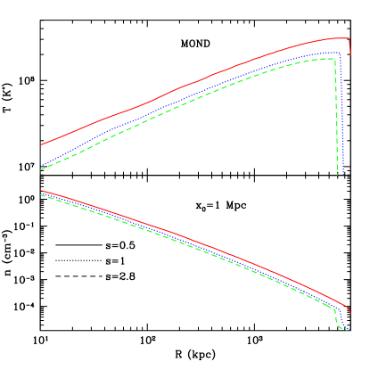
Figure 2: The temperature (top) and the density (bottom) profiles in MOND for $s=0.5$, 1 and 2.8, as indicated in the figure. The normalisation is such that the mean value of the density within a comoving distance $x_{0}=1\rm Mpc$ is the same at the initial time for all three values of $s$.

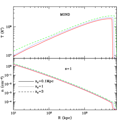
Figure 3: Profiles in MOND for $s=1$, but for three values of the normalisation as indicated in the figure by the parameter $x_{0}$.

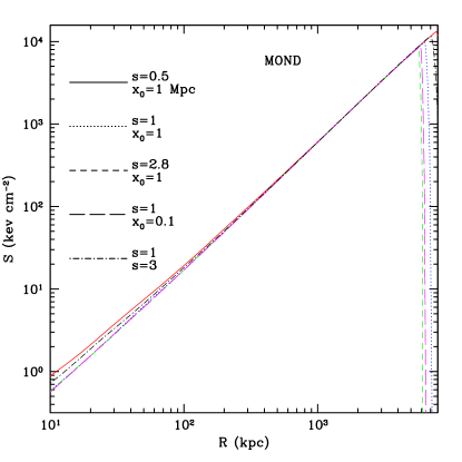
Figure 4: Entropy profiles in MOND at $z=0.1$ for various values of $s$ and $x_{0}$. The slope, $\,{\rm d}\ln S/\,{\rm d}\ln R$, at $R\lower 2.15277pt\hbox{$\;\buildrel>\over{\sim}\;$}10^{3}\rm kpc$ is 1.3, approximately.

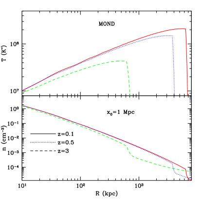
Figure 5: Profiles in MOND for $s=1$ and $x_{0}$ from outputs at three different redshifts, $z$, as indicated in the figure.

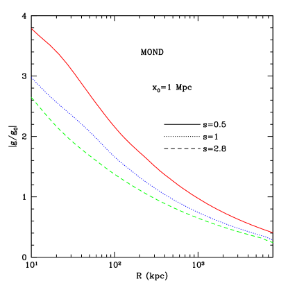
Figure 6: The ratio of the absolute value of the peculiar gravitational field relative to $g_{0}=1\times 10^{-10}\rm ms^{-2}$ as a function of radius for runs with the same normalisation and three different values of $s$.

6 The observational situation

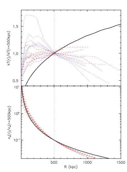
Figure 7: Top: MOND simulated temperature profiles (thick black line) compared to the individual profiles of clusters observed with XMM-Newton (red dashed lines) and Chandra (blue dotted lines). Bottom panel: MOND simulated density profiles (thick black line) shown with respect to the observed density profiles of nearby clusters by the XMM-Newton satellite (red dashed lines). In both panels the profiles have been normalised according to their respective values at $r=500$ kpc as marked radius by dotted vertical line.

We confront the temperature and density profiles of MOND with recent X-ray observations of galaxies clusters. We use the recently published temperature profiles by Pointecouteau et al. (2005) obtained for a sample of 10 nearby ($z<0.15$) clusters with the XMM-Newton satellite. To give a fair idea of the variation in shape of the observed temperature profiles, we also add the temperature profiles of eleven nearby ($z<0.23$) clusters obtained by Vikhlinin et al. (2004) with the Chandra satellite. Both samples cover a wide range of temperatures from 2 to 9 keV. We scale each temperature profile to its value at $500$ kpc (i.e $kT(r=500\textrm{~{}kpc})$) in order to compare them with our simulated profiles. To avoid any extrapolation, we kept only the 16 clusters which were observed beyond 500 kpc (i.e 8 XMM-Newton and 8 Chandra clusters). The scaled temperature profiles are shown in Fig. 7 (top panel).

We also compare the observed density profiles with MOND’s profiles. The observed profiles correspond to the parameterised form derived by fitting the X-ray surface brightness profile of each cluster. For this comparison, we only use the XMM-Newton profiles. The best fit models for the density profiles of the ten clusters from Pointecouteau et al. (2005) are plotted together with the MOND density profile in Fig. 7 (bottom panel). All profiles are scaled to their respective values at $500\;\rm kpc$.

All of the observed clusters are identified as relaxed and show small deviations from sphericity. The temperature drop towards the centre in the observed profiles is the result of cooling. Since cooling is not included in our simulations, we restrict the comparison to $R\lower 2.15277pt\hbox{$\;\buildrel>\over{\sim}\;$}200\;\rm kpc$.

For better visualisation, all profiles are scaled to their respective values at $R=500\;\rm kpc$. At that radius, the minimum, maximum, average, and median values of the observed temperature are (in $10^{7}{\rm K}$), 1.9, 11.9, 6.6, and 6.8, respectively. The corresponding values for the baryon number density are (in $10^{-4}\rm cm^{-3}$), 4.4, 20.6, 13.2, and 18.2, respectively. At this radius MOND yields a temperature range consistent with the observations. However, among the MOND runs of all values of $s$ and $x_{0}$ that we shown, the minimum value number density at $500\;\rm kpc$ is MOND density in MOND is $0.07\;\rm cm^{-3}$. This is substantially higher that the maximum observed number density of $0.0026\;\rm cm^{-3}$. More importantly, the temperature profile, $\sim r^{0.5}$, in MOND is, in clear contrast to the observed profiles, either flatten or show a mild decline in the outer regions. The entropy profile in MOND has a logarithmic slope of $\sim 1.5$, as compared to $0.94\pm 0.14$ and $0.95\pm 0.02$ found in the observations (Pratt & Arnaud 2005 and Piffaretti et al.  2005, respectively). This is another manifestation of the mismatch between temperature profiles in MOND and the observations.

7 Summary and discussion

In this paper we aimed at: (1) studying the density and temperature profiles of spherically symmetric perturbations evolved under MONDian gravity, and (2) comparing the predicted profiles with recent X-ray observations of the intracluster medium (ICM). A key finding here is that the profiles in MOND acquire a nearly universal shape independently of the initial fluctuations. This is in contrast to the Newtonian theory where the profiles are sensitive to the shape of the initial profiles. The shock radius in MOND is nearly independent of the amplitude of the initial perturbation while in the Newtonian case it is proportional to the amplitude (see Eq. 29).

The insensitivity to the initial density profile, leaves very little leeway in matching MOND predictions to observed properties of the ICM. In Newtonian dynamics, one can, to a great extent, resort to varying initial conditions to try to match the observations. In MOND one has to depend, almost entirely, on non-gravitational physical processes. One such process may be thermal conduction. The thermal conduction time scale is estimated as $R_{\rm c}\sim(2\kappa Tt/5nkT)^{1/2}$. Assuming a thermal conductivity, $\kappa$, of 0.2 times the Spitzer value $\kappa_{\rm Sp}=9.210^{-7}T^{5/2}\rm erg\;s^{-1}\;K^{-1}\;cm^{-2}$ (Spitzer 1962), we obtained $R_{\rm c}\sim 200\;\rm kpc$ for $t=14\;\rm Gyr$, $n=0.001\rm cm^{-3}$ (see Fig. 2 at $R=10^{3}\;\rm kpc$), and $T=5\times 10^{7}\;\rm K$. Therefore, thermal conduction can help, especially for the highest temperature clusters of $T\sim 10^{8}\;\rm K$. For $T\lower 2.15277pt\hbox{$\;\buildrel<\over{\sim}\;$}5\times 10^{7}\rm\;K$ conduction seems inefficient at producing the desired temperature profile. Note that we have used the cosmic time $t=t_{\rm H}\approx 14\rm\;Gyr$ to estimate $R_{c}$. In the outer regions one should actually take $t_{\rm H}-t_{\rm collapse}$ where $t_{\rm collapse}$ is the time at which these regions collapsed and shock-heated. According to Fig. 5 the shock radius have grown from $600\rm\;kpc$ at $z=3$ to $7000\rm\;kpc$ at $z=0$. The time interval between $z=3$ and $z=0$ is $t_{\rm H}-t_{\rm collapse}=0.25t_{\rm H}$ which reduces $R_{\rm c}$ by a factor of $2$. Non-gravitational heating of the ICM can also be invoked to alter the profiles, but it is hard to imagine a realistic mechanism that will flatten the temperature in the outer regions (e.g. Borgani et al. 2005).

Our findings as well as those of previous authors, pause some puzzles for MOND to overcome. While Newtonian dynamics has its own problems in matching the cluster data, the lack of dependence on the initial conditions, makes MOND harder to reconcile with these data.

8 Acknowledgements

We are deeply indebted to Alexey Vikhlinin for kindly providing his Chandra temperature profiles. AN thanks Tom Theuns for advice on the numerical code. AN is also grateful to Arif Babul and Scott Kay for many stimulating conversations. EP aknowledges the financial support of the Leverhulme Trust (UK).

References

- (1) Aguirre A., Schaye J., Quataert E., 2001, ApJ, 561, 550
- (2) Bekenstein J.D., Milgrom M., 1984, ApJ, 286, 7
- Bekenstein (2004) Bekenstein J. D., 2004, Phys. Rev. D, 70, 083509
- Bertone et al. (2004) Bertone G., Hooper D., Silk J., 2004, Phys. Rep., 405, 279
- (5) Binney J.J., Tremaine S., 1987, Galactic Dynamics, Princeton
- (6) Borgani S.., Finoguenov A., Kay S.T., Ponman T.J., Springel V., Tozzi P., Voit G.M., 2005, astro-ph/0504265
- (7) Chuzhoy L., Nusser A., 2000, MNRAS, 319, 797
- (8) de Blok W.J.G., McGaugh S.S., Bosma A., Rubin V.C., 2001, ApJL, 552, 23
- (9) Farrar G.R., Peebles P.J.E., 2004, ApJ, 604, 1
- (10) Felten J.E., 1984, ApJ, 286, 3
- (11) Gradwohl B.A., Frieman J.A., 1992, ApJ, 398, 407 [ISI]
- (12) Hayashi E., Navarro J.F., Power C., Jenkins A., Frenk C.S., White S.D.M., Springel V., Stadel J., Quinn, T. R., 2004, MNRAS, 355, 794
- (13) Kirkman D., Tytler D., Burles S., Lubin D., O’Meara J.M., 2000, ApJ, 529, 655
- (14) Knebe A., Gibson B.K., 2004, MNRAS, 347, 1055
- (15) Milgrom M., 1983, ApJ, 270, 365
- (16) Milgrom M., Braun E., 1988, ApJ, 334, 130
- (17) McGaugh S.S, 1999, ApJ, 523, L99
- (18) McGaugh S.S, 2004, ApJ, 611, 26
- (19) Mortlock D.J., Turner E.L., 2001, MNRAS, 327, 557
- (20) Nusser A., 2002, MNRAS, 331, 909
- (21) Nusser A., Gubser S.S., Peebles P.J., 2005, PhRvD 71h3505
- (22) Peebles J.P.E, 1980 Large Scale Structure, Princeton University Press
- Piffaretti et al. (2005) Piffaretti R., Jetzer P., Kaastra J. S., Tamura T., 2005, A&A, 433, 101
- (24) Pointecouteau E., Arnaud M., Pratt G. W., 2005, A&A, 435, 1
- (25) Pratt G. W., Arnaud M., 2005, A&A, 429, 791
- (26) Richtmyer R., Morton K.W., 1967, Difference Methods for Initial-Value Problems, New York: Interscience
- (27) Sanders R.H., 1998, MNRAS, 296, 1009
- Sanders (2001) Sanders R. H., 2001, ApJ, 560, 1
- (29) Spitzer L., 1962, Physics of Fully Ionized Gases, New York: Interscience
- (30) Sealfon C., Verde L., Jimenez R., 2005, PhRvD, 71h3004
- (31) Shirata A., Shiromizu T., Yoshida, N., Suto Y., 2005, PhRvD, 71f4030
- (32) Spergel D.N. et al., 2003, ApJS, 148, 175
- (33) Stachniewicz S., Kutschera M., 2004, astro-ph/0412614
- (34) The L.S., White S.D.M., 1988, AJ, 95, 1642
- (35) Thoul A.A., Weinberg D.H., 1995, ApJ, 442, 480
- (36) Vikhlinin A., et al., 2005, astro-ph/0412306