CLASS B0631+519: Last of the CLASS lenses

Abstract

We report the discovery of the new gravitational lens system CLASS B0631+519. Imaging with the VLA, MERLIN and the VLBA reveals a doubly-imaged flat-spectrum radio core, a doubly-imaged steep-spectrum radio lobe and possible quadruply-imaged emission from a second lobe. The maximum separation between the lensed images is 1.16 arcsec. High resolution mapping with the VLBA at 5 GHz resolves the most magnified image of the radio core into a number of sub-components spread across approximately 20 mas. No emission from the lensing galaxy or an odd image is detected down to 0.31 mJy (5$\sigma$) at 8.4 GHz. Optical and near-infrared imaging with the ACS and NICMOS cameras on the HST show that there are two galaxies along the line of sight to the lensed source, as previously discovered by optical spectroscopy. We find that the foreground galaxy at $z$=0.0896 is a small irregular, and that the other, at $z$=0.6196 is a massive elliptical which appears to contribute the majority of the lensing effect. The host galaxy of the lensed source is detected in the HST near-infrared imaging as a set of arcs, which form a nearly complete Einstein ring. Mass modelling using non-parametric techniques can reproduce the near-infrared observations and indicates that the small irregular galaxy has a (localised) effect on the flux density distribution in the Einstein ring at the 5-10% level.

1 Introduction

Strong gravitational lensing occurs when a background source is multiply imaged by the gravitational field of an intervening massive galaxy or cluster of galaxies. Observations of gravitational lenses have been used in many astrophysical applications, such as in modelling the mass distributions of distant galaxies and as constraints on cosmological models (Kochanek, Schneider & Wambsganss, 2004). CLASS (Cosmic Lens All-Sky Survey; Myers et al. 2003; Browne et al. 2003) and JVAS (Jodrell Bank - VLA Astrometric Survey; Patnaik et al. 1992; Browne et al. 1998; Wilkinson et al. 1998) are radio surveys of the northern sky designed to find gravitationally lensed compact radio sources. In JVAS and CLASS 11685 sources in a statistically well-defined sample have been examined and 22 lens systems found. In this paper, we announce the discovery of the last of these systems, CLASS B0631+519. This lens system exhibits complex radio structure over scales from 3.6 mas to 1.16 arcsec and has a nearly complete infrared Einstein ring, similar to that in B1938+666 (Patnaik et al., 1992; King et al., 1997, 1998). It is a system with one of the richest lensed image structures known and is thus an ideal system with which to probe mass properties of the lensing galaxy. B0631+519 is a member of the CLASS statistically complete sample.

In Section 2 we discuss radio observations of B0631+519 made using the Very Large Array (VLA), Very Long Baseline Array (VLBA) and the Multi-Element Radio-Linked Interferometer Network (MERLIN; Thomasson 1986). Section 3 presents optical and near-infrared images taken with the William Herschel Telescope (WHT) and the Hubble Space Telescope (HST). In Section 4 we consider the data in the context of the lens hypothesis and test some simple lens models, and in Section 5 we conclude by discussing the future priorities for work on this lens.

2 Radio observations

As described in Myers et al. (2003) and Browne et al. (2003), potential lens candidates from CLASS are tested by observing them with a range of angular resolutions and at several different frequencies. If the supposed multiple images in a lens candidate are found to have very different surface brightnesses at any angular resolution the lens hypothesis can usually be rejected immediately, since lensing preserves surface brightness. In CLASS, candidates discovered with the VLA are observed with higher resolution using MERLIN, and, if not eliminated at this stage, are re-observed with even higher resolution using the VLBA. Accordingly, radio observations of B0631+519 have been made over frequencies ranging from 1.7 GHz to 15 GHz, with angular resolutions from 3.6 mas to 236 mas. The observations are summarised in Table 1.

Date observed	Instrument	Frequency [GHz]	Integration time	Map residual noise [$\mu$Jy beam-1]	Mean beam size [mas]
1994 March 05	VLA	8.4	16 sec	410	234
1999 July 02	VLA	15	354 sec	360	142
1999 August 03	VLA	8.4	510 sec	86	236
1999 December 10	VLBA	1.7	1.4 hr	130	8
2001 March 21	VLBA	5	1.7 hr	82	3.6
2001 July 07	MERLIN	5	19 hr	120	52
2002 December 01	VLBA	1.7	7.8 hr	64	9
2003 March 01	MERLIN	1.7	20 hr	62	173

Table 1: Radio observations made of B0631+519 to date.

2.1 VLA

B0631+519 was observed at 8.4 GHz on 1994 March 05 and 1999 August 03. The 1999 observation was a follow-up to the 1994 snapshot observation and had almost 5 times its sensitivity (Table 1). The snapshot was made using a bandwith of 50 MHz, and 3C48 was used to set the flux density scale; the follow-up observation used a bandwidth of 100 MHz, and the flux density scale was set using 3C147.

All VLA observations of B0631+519 were made with the VLA in ‘A’ configuration, and were calibrated using aips and mapped with the Caltech difference mapping program difmap (Shepherd, 1997). Model component positions and flux densities from the VLA observations are displayed in Table 2.

The deconvolved map from the 1999 follow-up observation is shown in Figure 1. We label the detected radio components as shown in Figure 1. Components A1 and B are separated by 1.15 arcsec at a position angle (from brightest to dimmest source) of $+$135$\degr$, and the A1:B flux density ratio is 8:1. Components A1, A2 and B are unresolved. Component X is a knot of elevated surface brightness embedded in the jet- or arc-like feature that branches to the south of A2. There is some extended emission visible on the opposite side of A1 from X, which we label Y, although the detection is marginal (about 2.3$\sigma$). The total flux density in the model is 42$\pm$2 mJy (where we have assumed 5% errors on absolute flux density measurements from the VLA at 8.4 GHz).

In the snapshot A1, A2 and B were detected, while X and Y were not. The snapshot shows an A1:B flux density ratio of about 7:1, and a total flux density from the candidate of 46$\pm$2 mJy. This is 10% higher than the equivalent quantity in the follow-up map. The discrepancy might be accounted for by uncertainty in the absolute amplitude calibration between the 1994 and the 1999 observations, but it could also indicate that the source is variable. The mean size of the synthesized beam varies by less than 3 mas between the two (uniformly weighted) maps, or by 2% in area, so it is unlikely that 10% of the emission has been resolved out in one map with respect to the other. The A1:B flux density ratio also changes by 16% between the two observations, which is hard to reconcile with a global mis-calibration of the amplitude scale. The signal-to-noise ratios on A1 and B were at least 10 in all VLA observations.

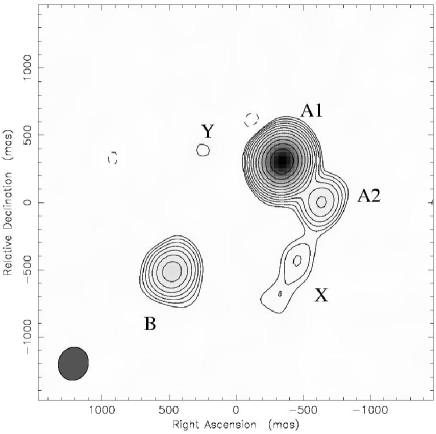
Figure 1: Radio map of the VLA 8.4 GHz data taken on 1999 August 03. The RMS noise in the residual map is 86 $\mu$Jy beam^-1. The data are naturally weighted. The synthesized beam is sized 250$\times$223 mas with the major axis oriented along a position angle (P.A.) of $-$17.5$\degr$. The lowest contours are plotted at -3 and 3 times the RMS noise level; successive contours represent an multiplicative increase in surface brightness by a factor of 1.5, up to the highest contour level of 22.8 mJy beam^-1. Component A1 is located at RA: 06^h 35^m 12.31402^s, Dec: $+$51$\degr$ 57’ 01.8026″(J2000.0) as measured by the VLBA.

A further observation of B0631+519 was made with the VLA at 15 GHz on 1999 July 02 for 354 seconds, with a bandwidth of 100 MHz. The amplitude scale was set with observations of 3C286. The deconvolved, naturally weighted map is shown in Figure 2. The total flux density detected at 15 GHz is 34$\pm 3$ mJy, and the A1:B flux density ratio is 7.5:1. Both A1 and B are unresolved by the VLA at this frequency. A2 is not detected, suggesting that it has a steeper spectral index than A1 and B.

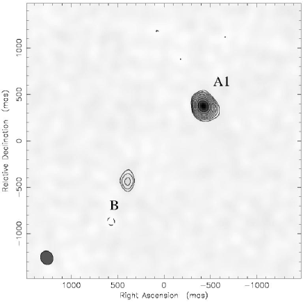
Figure 2: 15 GHz VLA data taken on 1999 July 02. The synthesized beam is 152$\times$132 mas oriented with the major axis at a P.A. of $+$26$\degr$, and the RMS noise in the residuals is 360 $\mu$Jy beam^-1. The data are naturally weighted. Contours are plotted as for Figure 1; the highest contour value is 27.8 mJy beam^-1.

Component	Frequency [GHz]	Position offsets [mas]		Flux density [mJy]
		$\Delta$R.A.	$\Delta$Dec.
A1	8.4	$+$0$\pm$1	$+$0$\pm$1	34.3$\pm$1.7
	15	$+$0$\pm$2	$+$0$\pm$2	29.6$\pm$3
A2	8.4	$-$297$\pm$10	$-$300$\pm$10	2.2$\pm$0.1
	15	-	-	$<$1.8
B	8.4	$+$819$\pm$5	$-$819$\pm$5	4.2$\pm$0.2
	15	$+$813$\pm$19	$-$805$\pm$19	3.95$\pm$0.4
X	8.4	$-$114$\pm$33	$-$754$\pm$33	0.98$\pm$0.1
	15	-	-	$<$1.8
Y	8.4	$+$577$\pm$70	$+$81$\pm$70	0.2$\pm$0.1
	15	-	-	$<$1.8

Table 2: Model components from radio observations of B0631+519 with the VLA. All position offsets are relative to A1. The 8.4 GHz flux densities and positions are derived from the 1999 follow-up data, not the 1994 discovery data. Non-detections are quoted at the 5$\sigma$ level throughout this paper. Errors on positions of Gaussian model components are estimated by dividing the beam size by the peak signal-to-noise ratio (SNR). Errors on flux densities are assumed to be subject to a 5% random error in absolute flux density calibration at 8.4 GHz and a 10% error at 15 GHz.

2.2 MERLIN

B0631+519 was observed at 5 GHz using MERLIN on 2001 July 07, over a period of 19 hours. Telescope gains were calibrated using the source OQ208, and the observations were phase referenced to the source JVAS J0642+5247. All MERLIN data were reduced by initial amplitude calibration and flagging with the MERLIN D-programs, followed by phase and amplitude calibration and further flagging in aips. difmap was used to map and self-calibrate the data. 3C286 was used to set the flux density scale for all MERLIN observations. Model component positions and flux densities from the MERLIN observations are shown in Table 3.

The deconvolved 5 GHz map is shown in Figure 3. Component B has been resolved into two components (B1 and B2). A1 and B1 appear compact, but A2 and B2 are slightly resolved. X and Y have been resolved out and there is no sign of the extended emission revealed by the 8.4 GHz VLA observations.

Figure 3: Radio map of the 5 GHz MERLIN observations taken on 2001 July 07. The data were naturally weighted. The beam size is 58$\times$46 mas with the beam’s major axis being oriented at a P.A. of $-$34$\degr$. The RMS noise in the residuals is 120 $\mu$Jy beam^-1. Contours are plotted at levels of (-3, 3, 4.5, 6.75, 10.1, 15.2, 22.8, 34.2, 51.3, 76.9, 115, 173, 259) times the RMS noise.

Additional MERLIN observations were made at 1.7 GHz on 2003 March 01. Phase referencing was carried out using the source J0636+5009. B0552+398 was used to calibrate the telescope gains. The newly upgraded 76 metre Lovell Telescope was included in the interferometer network, allowing an RMS noise level in the deconvolved map of 62 $\mu$Jy beam^-1to be reached in 20 hours. The deconvolved 1.7 GHz map is shown in Figure 4. The map shows emission both to the west and east of image A1. We identify these regions of emission as low-frequency counterparts to components X and Y seen in the VLA data. B1 also develops an extension to the west, which we label Z.

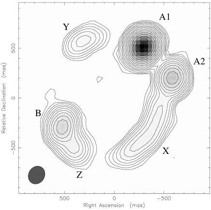
Figure 4: Radio map of the 1.7 GHz MERLIN observations taken on 2003 March 01. The data were naturally weighted. The synthesized beam is sized 186$\times$161 mas at P.A. $-$31.7$\degr$. Contours are plotted at factors of (-3, 3, 4.5, 6.75, 10.1, 15.2, 22.8, 34.2, 51.3, 76.9, 115, 173, 259, 389, 584, 876) times the RMS noise.

Component	Frequency [GHz]	Position offsets [mas]		Flux density [mJy]
		$\Delta$R.A.	$\Delta$Dec.
A1	1.7	$+$0$\pm$1	$+$0$\pm$1	66.4$\pm$6.6
	5	$+$0$\pm$1	$+$0$\pm$1	46.9$\pm$4.7
A2	1.7	$-$293$\pm$1	$-$313$\pm$1	19$\pm$1.9
	5	$-$293$\pm$3	$-$308$\pm$3	4.2$\pm$0.4
B	1.7	$+$809$\pm$1	$-$800$\pm$1	11.8$\pm$1.2
B1	5	$+$828$\pm$1	$-$816$\pm$1	5.4$\pm$0.5
B2	5	$+$801$\pm$8	$-$722$\pm$8	1.3$\pm$0.1
X	1.7	$-$40	$-$880	11$\pm$1
	5	-	-	$<$0.6
Y	1.7	$+$595$\pm$6	$+$67$\pm$6	2.7$\pm$0.3
	5	-	-	$<$0.6
Z	1.7	$+$691$\pm$5	$-$1016$\pm$5	5.0$\pm$0.5
	5	-	-	$<$0.6

Table 3: Radio components detected in B0631+519 with MERLIN. All position offsets are relative to A1. X is a large arc that is not well described by a single gaussian component; the position quoted is an estimate for the centre of the feature. The integrated flux density of X was derived by summing within the 3$\sigma$ contour. We have assumed a 10% absolute calibration error on flux densities from MERLIN. Position errors are estimated from the beam size divided by the peak SNR.

2.3 VLBA

The VLBA was used to observe B0631+519 at 5 GHz on 2001 March 21 over a period of 1.7 hours. Data were taken using four contiguous 8 MHz bands and a single hand of circular polarisation. The observations were phase-referenced using the calibrator source J0631+5311 and employed 2 bit sampling during digitisation; correlation was performed using the VLBA correlator in Socorro. During correlation each band was subdivided into 16 0.5 MHz channels and the data were averaged into 2 s integrations.

All VLBA observations were reduced using aips to flag and calibrate the data, following standard recipes for the VLBA. The aips task scimg was then used to map the data through cycles of CLEAN (Högbom, 1974) followed by self-calibration. Flux densities and positions of VLBA components are shown in Table 4.

The deconvolved 5 GHz maps are shown in Figure 5. Uniform weighting was employed. The resolution achieved was 3.6 mas, sufficient to split A1 into four sub-components (labelled A1a to A1d) spread over an angle of about 20 mas. B1 remained unresolved, and no emission from the A2, B2, X, Y or Z components was detected down to the 5$\sigma$ limit of 390 $\mu$Jy beam^-1, indicating that these components have probably been resolved out.

We note that the sum of the flux densities of components A1a to A1d (46$\pm$2 mJy) is consistent with the MERLIN 5 GHz flux of component A1 to within the measurement errors, which implies both that A1 did not vary by more than 5% over the 4 months separating the observations and also that no radio structure seen in A1 by MERLIN was resolved out by the VLBA, despite the factor of $\sim$14 increase in resolution. However, another possible explanation is that an increase in source flux density (due to intrinsic variability) cancelled out any loss of emission due to resolution effects. The same conclusions and caveats apply to the MERLIN and VLBA observations of B1 at 5 GHz.

Comparison of the total A1 flux density to the flux density of B1 suggests an A1:B1 magnification ratio of $\sim$9:1, and hence that sub-components in B1 corresponding to those in A1 would span about 2 mas. Resolving the expected sub-components in B1 is thus well within the capabilities of VLBI (Very Long Baseline Interferometry).

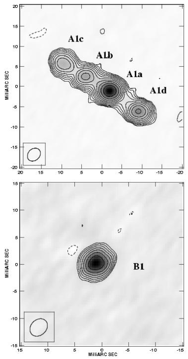
Figure 5: Radio map of the 5 GHz VLBA observations taken on 2001 March 21, showing image A (top) and image B (bottom). The data were uniformly weighted. The beam-size is 3.8$\times$3.4 mas oriented at P.A. $+$144$\degr$ and the RMS noise is 82 $\mu$Jy beam^-1. Contours are plotted at levels of (-3, 3, 4.5, 6.75, 10.1, 15.2, 22.8, 34.2, 51.3) times the RMS noise.

Two epochs of phase-referenced VLBA data were obtained at 1.7 GHz, on 1999 December 10 and 2002 December 01. The phase reference source used was J0631+5311. The 1999 data was taken in two polarisations via 4 contiguous bands, 2 bands to each polarisation. 2-bit sampling was used, and correlation at Socorro again subdivided each band into 16 0.5 MHz wide channels and averaged the data into 2 s integrations. The phase centre was taken halfway between images A1 and B1 to minimise bandwidth smearing.

The CLEANed, naturally weighted maps of A1, A2 and B1/B2 from the 2002 epoch are shown in Figure 6. A1 appears resolved but (unsurprisingly) smoothed compared to the 5 GHz VLBA map, while B1 remains unresolved. A2 is resolved into an arc-like feature of low surface brightness that extends over 80 mas. B2 is partially resolved into an extended source. No emission was detected from components X, Y or Z.

The maps from the two 1.7 GHz epochs look very similar. The flux densities of A1, A2 and B2 agree between the two epochs to within the measurement errors. The flux density of B1 decreases by about 9% between 1999 and 2002; this decrease is not quite significant at the 2$\sigma$ level given the measurement errors of about 5% for B1’s flux density. The measurements of the A1/B1 image separation from the two epochs are consistent to within 0.5 mas, while the A1-B2 separation measurements agree to within 2 mas.

To identify which of the four VLBA sub-components of A1 correspond to the flat-spectrum radio core in the lensed source, we registered the 1.7 GHz map (from the 2002 epoch) with the 5 GHz map by using the position of component B1 as a reference (since B1 is largely unresolved in both maps). To overlay B1 in this way required the 1.7 GHz image to be translated by 1.7 mas south and 8.9 mas east because slightly different positions were used for the phase reference source J0631+5311 between the 5 GHz and 1.7 GHz observations. The translated 1.7 GHz map is shown overlaid on the 5 GHz map in Figure 7. Sub-component A1a appears to be the flat spectrum core, while the peak in the 1.7 GHz map corresponds to component A1c. Therefore at 5 GHz we apparently see both approaching and receding jets in the source AGN.

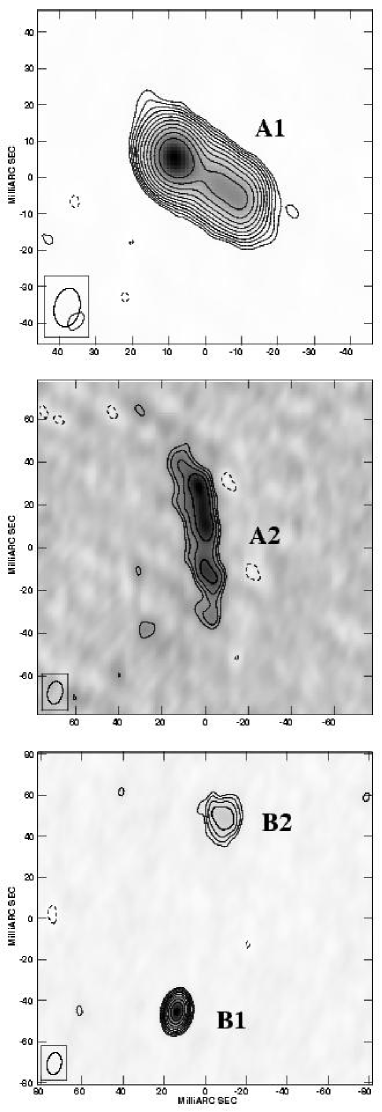
Figure 6: Radio maps of the 1.7 GHz VLBA observations taken on 2002 December 01. The data were naturally weighted. The synthesized beam is an elliptical gaussian sized 11.2$\times$7.5 mas oriented with its major axis at a P.A. of $+$177$\degr$. The RMS noise is 64 $\mu$Jy beam^-1. Contours are plotted at levels of (-3, 3, 4.5, 6.75, 10.1, 15.2, 22.8, 34.2, 51.3, 76.9, 115, 173) times the RMS noise.

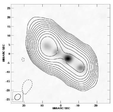
Figure 7: The 1.7 GHz VLBA observations from 2002 December 01 plotted with the 5 GHz data from the same instrument. The 5 GHz data are shown in greyscale, while the 1.7 GHz data are shown contoured (with the same contour levels as in Figure 6).

Component	Frequency [GHz]	Position offsets [mas]		Flux density [mJy]
		$\Delta$R.A.	$\Delta$Dec.
A1	1.7	$+$0$\pm$0.1	$+$0$\pm$0.1	51.4$\pm$3
A1a	5	$+$0$\pm$0.1	$+$0$\pm$0.1	20.5$\pm$1
A1b	5	$+$5.7$\pm$0.1	$+$3.5$\pm$0.1	8.8$\pm$0.4
A1c	5	$+$11.1$\pm$0.1	$+$6.6$\pm$0.1	7.3$\pm$0.4
A1d	5	$-$7.2$\pm$0.1	$-$5.0$\pm$0.1	9.2$\pm$0.5
A2	1.7	$-$300	$-$306	6.6$\pm$0.7
	5	-	-	$<$0.39
B1	1.7	$+$812.5$\pm$0.1	$-$827.5$\pm$0.1	5.6$\pm$0.3
	5	$+$822.5$\pm$0.1	$-$821.5$\pm$0.1	5.1$\pm$0.3
B2	1.7	$+$790.7$\pm$0.4	$-$732.9$\pm$0.5	2.2$\pm$0.2
	5	-	-	$<$0.39

Table 4: Model components for the radio observations of B0631+519 with the VLBA. Stated errors on flux densities assume a 5% random error in the absolute flux density scale calibration at the VLBA. The 1.7 GHz position offsets are given relative to the surface brightness peak in A1. For A2 and B2 at 1.7 GHz, we have doubled the error to reflect the uncertainty in the flux densities of these resolved components; their flux densities were obtained by summing within the 3$\sigma$ contour. Positions for A1, B1 and B2 were determined from the best-fit gaussians, restricted to the compact north-eastern feature in the case of A1 at 1.7 GHz. The position given for A2 is that of the brightest pixel. For the 5 GHz data, position offsets are taken relative to A1a at RA: 06^h 35^m 12.31390^s, Dec: +51$\degr$ 57’ 01.7949″(J2000.0).

2.4 Radio spectra from continuum data

We plot the radio spectra for the model components as a function of frequency in Figure 8. If the lens hypothesis is correct then all the lensed images of a source should have similar spectra, provided that the lens galaxy ISM does not scatter or absorb the source light, and that the source flux density is constant (Kochanek & Dalal, 2004). A1 and B1 have similar spectra, as do A2 and B2. Possibly X, Y and Z also have similar spectra, although at 8.4 GHz component Y is a marginal detection and component Z is a non-detection (we have plotted a 5$\sigma$ upper limit). We suggest that there are three separate source regions revealed by the radio observations, two of which are doubly-imaged and one of which is quadruply imaged (generating images Y, Z and the arc X). We will discuss the geometry of the source with respect to the lens caustics further in Section 4.

Figure 8: Plot of the radio spectra of the various radio components identified in B0631+519. The total flux density is based on measurements at 327 MHz from WENSS (Rengelink et al., 1997), at 1.4 GHz from NVSS (Condon et al., 1998) and at 5 GHz from the GB6 survey (Gregory et al., 1996).

3 Optical observations

Typically lens galaxies are radio-quiet ellipticals, so optical/infrared imaging is necessary to establish the lens galaxy position when the lenses are identified through radio searches. The position of the lens galaxy with respect to the lensed images can be used to constrain mass models, and in some systems unique information on the lensed source is available through optical imaging, for instance where an optical or infrared Einstein ring is visible as seen in CLASS B1938+666 (King et al., 1997, 1998). We have observed B0631+519 at optical/near-infrared wavelengths with the WHT through an R-band filter and with the HST through F555W, F814W and F160W filters. Details of these observations are listed in Table 5.

Instrument	Detector	Date observed	Filter	Integration time [sec]	PSF FWHM [arcsec]	Plate scale [arcsec pixel-1]
HST	ACS/WFC	2003 August 19	F555W	2236	0.05	0.05
HST	ACS/WFC	2003 August 19	F814W	2446	0.08	0.05
HST	NICMOS/NIC2	2004 February 15	F160W	2560	0.13	0.075
WHT	Aux. port CCD	2002 February 03	R	1800	0.7-0.9	0.108

Table 5: Optical and infrared observations made of B0631+519 to date.

3.1 WHT observations

B0631+519 was observed with the 4.2 metre William Herschel Telescope (WHT) on 2002 February 03, through an R-band filter. The detector used was a 1024$\times$1024 pixel TEK CCD, having a total field of view of 111 $\times$ 111 arcsec. The data were calibrated using the Starlink package ccdpack. B0631+519 was partially resolved, but there was insufficient resolution to separate any lensed images from the lens galaxy.

Aperture photometry was undertaken on the WHT image using observations of Landolt standard stars 93 407 and 100 280 (Landolt, 1992) to correct for atmospheric extinction and to calibrate the brightness scale in magnitudes. An elliptical aperture with major diameter 4.3 arcsec and an axis ratio of 0.75 was used to obtain an R-band magnitude for B0631+519 of 21.1$\pm$0.1, corrected for Galactic extinction using the dust maps of Schlegel, Finkbeiner & Davis (1998).

3.2 HST optical and near-infrared observations

B0631+519 was observed with the Hubble Space Telescope (HST) on 2003 August 19 and 2004 February 15 as part of HST proposal 9744, “HST Imaging of Gravitational Lenses” (PI: C.S. Kochanek). Images were taken using the Advanced Camera for Surveys (ACS) Wide Field Channel (WFC) through the F555W and F814W filters. B0631+519 was also observed with the NICMOS camera NIC2 through the F160W filter, in the MULTIACCUM observing mode. The wideband HST filters F555W, F814W and F160W approximately correspond to Johnson V, I and H respectively. Details of the optical observations are shown in Table 5. The ACS observations used a dither pattern consisting of two pointings separated by 0.73 arcsec. Two exposures were taken at both pointings to simplify cosmic ray rejection. The NICMOS data used a four-point dither pattern that placed B0631+519 at the centre of each quadrant of NIC2 in turn.

The ACS and NICMOS data were debiased, dark-subtracted and flat-fielded using the OTFR (On-The-Fly-Recalibration) facility of the MAST HST archive. We then used the multidrizzle script (Koekemoer et al., 2002) from within PyRAF to correct the ACS data for distortion, to eliminate cosmic rays and to combine dithered pointings into a single output frame, the shifts between frames being obtained from application of cross-correlation through the crossdriz task in IRAF. The NICMOS data were combined using pydrizzle to interpolate the data onto an output image with a uniform pixel scale of 0.075 arcsec, using the standard distortion solution for NIC2. Cosmic rays in the NICMOS data were identified and blanked by the OTFR pipeline itself. The IRAF  task pedsub was used to remove some residual dark signal that was evident in the output from the pipeline. Both the ACS and NICMOS images were aligned to the local celestial coordinate axes as part of the drizzling process.

The HST images (Figure 9) reveal two galaxies at the lens system position, surrounded by arcs of emission from the lensed source at longer wavelengths. We label these galaxies L1 and L2. L1 appears to be an elliptical galaxy, and is detected in all three bands. In the F814W and F160W images some emission from the source appears in the form of arcs of extended emission encircling L1, consistent with the lens hypothesis if L1 is the primary lensing galaxy. L2 appears to be an irregular galaxy and is seen in the F555W and F814W data, although in the latter it is confused with one of the lensed arcs. L2 is not cleanly detected in the NICMOS image, and may not be visible in the near-infrared.

The ACS images have a large enough field of view to show the environment of B0631+519. The nearest extended object is located 4.4 arcsec away at a P.A. of -72°, and has a total I_mag $\sim$ 22.3 in a 4 arcsec diameter aperture. The object’s light distribution is not smooth and is difficult to classify.

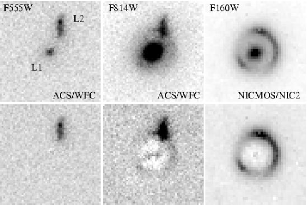
Figure 9: HST images of B0631+519. The top row of images show the lens before subtraction of L1, while the bottom row shows the residuals after subtraction of the best-fit Sérsic profile. North is up and east is left. The images are 3$\times$3 arcsec in size, and are centred on L1.

We carried out surface-brightness fitting on L1 using a Sérsic light profile (Sérsic, 1968) convolved with appropriate PSFs produced by TinyTim (Krist, 1993). The profile parameters were varied to minimise the sum of squared residuals between the data and the model. When fitting L1’s surface-brightness profile we masked out L2 and the lensed images to avoid disturbing the fit. L2 and the lensed arcs do not have easily parametrizable surface light distributions, so we did not attempt to separate them in the F814W or F160W images, and report only the sum of light remaining after subtraction of L1. In the F555W image the arcs were not detected, so we used gaia to fit an elliptical aperture to L2 (after L1 had been subtracted). The centroid of L2 was found to be $-$0.33 arcsec east and $+$0.74 arcsec north of L1. The axis ratio of the best-fit aperture was 0.56, with the major axis having a position angle $-$1.1°east of north. Table 6 shows the properties of the Sérsic profiles subtracted from L1.

Parameter	Filter
	F555W (V)	F814W (I)	F160W (H)
Offset in R.A. [mas]	$+$360$\pm$80	$+$380$\pm$80	$+$360$\pm$80
Offset in Dec. [mas]	$-$500$\pm$80	$-$530$\pm$80	$-$500$\pm$80
Total magnitude	22.7	20.0	17.7
Effective radius [mas]	540	560	550
Ellipticity	0.09	0.17	0.12
Position angle	$-$48	$-$53	$-$57
Power-law index	0.29	0.28	0.30

Table 6: Parameters of the best-fit Sérsic profiles fitted to L1 in the three HST images. A power-law index of 0.25 corresponds to a de Vaucouleurs surface-brightness profile. The total magnitudes are specified in the Johnson photometric system, corrected for galactic extinction. Position offsets are given relative to image A1.

The ACS and NICMOS images following subtraction of L1 are shown in Figure 9. The Sérsic profile is a reasonable fit to the HST data, leaving maximum residuals of 3% and 4% of L1’s peak brightness in the case of the F814W and F160W images respectively. The residuals are undetectable within the noise in the case of the F555W image, which has the lowest signal-to-noise ratio of all the HST observations.

Source	Brightness
	V	R	I	H
Total	22.1$\pm$0.1	21.1$\pm$0.1	19.9$\pm$0.1	17.3$\pm$0.1
L1	22.8$\pm$0.1		20.0$\pm$0.1	17.8$\pm$0.1
L2	23.0$\pm$0.1			$>$23
L2+images			22.3$\pm$0.1
Images	$>$25			18.3$\pm$0.1

Table 7: Results of photometry on B0631+519. The figures reported in this table were measured within a circular aperture of 4 arcsec diameter. For the total luminosity of the subtracted Sérsic models see Table 6. The WHT R-band magnitude was calculated using a Kron elliptical aperture 4.3 arcsec in (major axis) diameter. All figures have been corrected for galactic and, in the case of the WHT, atmospheric extinction. Non-detections are reported as lower limits on magnitude at the 5$\sigma$ level.

We carried out aperture photometry on B0631+519, using a circular aperture 4 arcsec in diameter to measure the flux of the lens system as a whole, of the Sérsic model for L1 and of whatever light remained after subtraction of the Sérsic model from the data. The measurements were converted into the Johnson magnitude system using published zero points for HST magnitude systems. Galactic extinction was estimated from Schlegel, Finkbeiner & Davis (1998). The results are shown in Table 7. The differences in L1 magnitudes between Tables 6 and 7 are due to the fact that the values given in the latter are sums of the flux within finite apertures, while those in the former are equivalent to sums within infinite apertures.

The lens galaxy position with respect to the lensed images, when known, provides two constraints on simple parametric lens models under the assumption that the centre of (smoothly distributed) light and the centre of mass for a galaxy are coincident. Since the lens galaxy in B0631+519 is apparently radio-quiet, the radio and HST data must be overlaid as accurately as possible to establish the lens position. The lensed images at near-infrared and optical wavelengths exhibit no obvious point-like components that could be unambigiously aligned with the radio structure. We must therefore rely on absolute astrometric calibration based on stars visible in the field to align the optical and near-infrared images with radio data.

We used the 2MASS catalogue with Starlink’s gaia to establish an astrometric calibration for the ACS images (F555W and F814W filters). 2MASS positions have no significant systematic offsets with respect to the radio-based ICRF (da Silva Neto et al., 2005). The astrometric solutions were based on twelve star positions and had reported RMS errors of $\pm$0.08 arcsec in R.A. and declination, although examination of objects around the field indicated positional agreement between the two calibrated images to within 0.05 arcsec. In the case of NICMOS the relatively small field of view (19.5$\times$19.5 arcsec) meant that only one star near to B0631+519 was imaged. The centre of this star was used as a reference to fix the absolute astrometry for the image. We estimate the astrometric error in the resulting solution for the drizzled NICMOS image at 0.08 arcsec, since the star’s position on the sky was derived from the astrometrically calibrated ACS F555W image. The rotation of the image was checked by calculating the position angle of the vector from the field star to L1’s position. This angle agreed with the same quantity measured from the ACS images to within 0.05°. Figure 10 shows the 1.7 GHz MERLIN map overlaid on the ACS and NICMOS images.

Fitting Sérsic profiles to L1 gave us best-fit pixel positions for the galaxy centre in all three HST filters, which we converted into celestial coordinates using the absolute astrometric solutions from the HST images. The sky position of image A1 (from the 1.7 GHz VLBA observations) was then subtracted to leave L1’s offset on the sky from A1. These offsets are reported in Table 6. The agreement between the offsets from the F555W and F160W images (which effectively share the same astrometric solution) and the disagreement between F555W and F814W suggests that the error in the galaxy position is dominated by the random error in the astrometric solutions for F555W and F814W; error contributions from the galaxy subtraction procedure and from the distortion solutions for each camera are negligible by comparison. The mean offset from A1 to L1 (based on the ACS data only) is $+$0.37$\pm$0.08 arcsec in R.A. and $-$0.52$\pm$0.08 arcsec in declination.

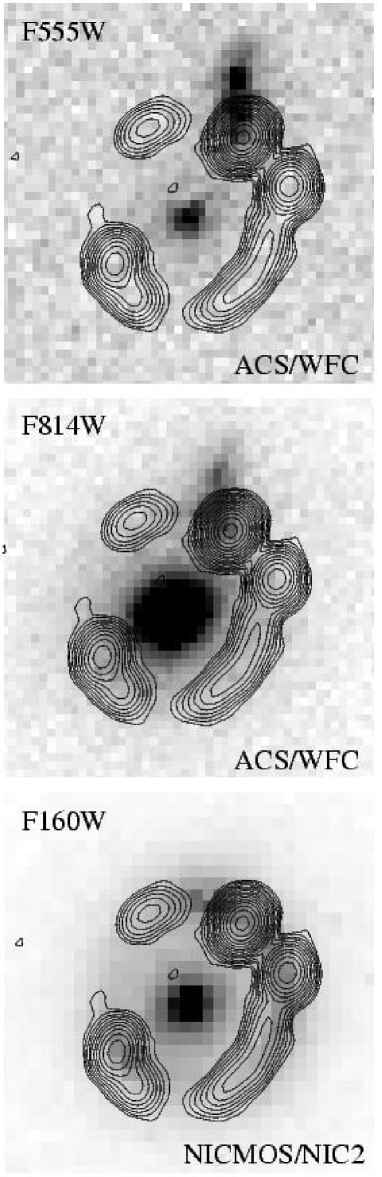
Figure 10: The MERLIN 1.7 GHz radio data (contoured) overlaid on the NICMOS and ACS images (greyscale). The ACS images cover 2.45$\times$2.45 arcsec, while the NICMOS image covers 2.475$\times$2.475 arcsec. All images are centred on L1. North is up and east is left.

3.3 Redshift-dependent properties of B0631+519

McKean et al. (2004) have obtained an optical spectrum of B0631+519 with the W. M. Keck telescope. They report the discovery of two distinct galaxies at two different redshifts. The first is an emission line galaxy at $z$=0.0896$\pm$0.0001; and the second, which is the dominant source of emission in the spectrum, is an elliptical galaxy at $z$=0.6196$\pm$0.0004. These spectral classifications are consistent with the morphologies, colours and flux densities of the two foreground galaxies detected in the HST imaging. Therefore, we associate the $z$=0.0896 emission line galaxy with L2, and the $z$=0.6196 elliptical with L1. McKean et al. (2004) refer to these galaxies in redshift order as G1 and G2 respectively; in this paper we have swapped the name order because the HST imaging demonstrates that L1 (G2) is the primary lensing galaxy, something that was not obvious from the spectroscopy alone.

McKean et al. (2004) also discuss the tentative detection of a single emission line from the lensed source at 5040Å. Assuming that the line is either due to Ly$\alpha$ or Mg II emission, they suggest 3.14 or 0.80 for the source redshift, respectively. However, further spectroscopy will need to be carried out to test these possibilities. We do not have enough (unambiguous) photometric information on the lensed images to attempt to choose between these possibilites by using photometric redshift techniques, but, in the absence of further spectroscopy, we can attempt to constrain the source redshift by determining the rest-frame luminosity $L$ of L1 and converting it into a velocity dispersion $\sigma$ using the fundamental plane of elliptical galaxies (Djorgovski & Davis, 1987; Dressler et al., 1987). This approach has been used before by Tonry & Kochanek (2000) to estimate the source redshift in CLASS B1938+666.

We converted the apparent magnitudes of L1 and L2 as measured by the HST (after translation into Johnson filters V, I and H, and following application of extinction corrections) into absolute magnitudes measured in Johnson B using

$$M_{B}=m_{Q}-5\log\left(\frac{D_{L}(z)}{10pc}\right)-K_{BQ}(z),$$ (1)

where $M_{B}$ is the predicted absolute magnitude of the object in B, $m_{Q}$ is the apparent magnitude of the object in some filter Q, $D_{L}(z)$ is the luminosity distance to the object at redshift $z$ and $K_{BQ}(z)$ is the K-correction from the object’s redshift and filter Q to the rest-frame in B. We adopt the redshifts of McKean et al. (2004) for L1 and L2. The K-corrections were calculated using the synphot package in IRAF, together with template spectra for L1 and L2 from Bruzual & Charlot (1993) and Kinney et al. (1996).

The K-correction for L1 was obtained from the model elliptical galaxy spectra of Bruzual & Charlot (1993), who provide multiple templates with various star formation histories and initial mass functions (IMFs). We selected the template that produced the lowest scatter in the predicted rest-frame B magnitudes for L1 amongst the three filters (F555W, F814W and F160W). The optimum template gave an RMS scatter amongst the three filters of $\sim 0.02$ mag, and was generated assuming a Salpeter IMF with mass range from 0.1 to 125 $M_{\odot}$, in which star formation took place $>$5 Gyr ago during a burst lasting 1 Gyr. The templates were used solely to obtain a spectral K-correction; no correction for luminosity evolution was applied.

The K-correction for L2 was estimated using the starburst galaxy spectrum templates of Kinney et al. (1996). Since there are several templates provided, each having differing amounts of internal extinction, we again selected the template that produced the lowest scatter in the predicted rest-frame B magnitudes for L2, but between the F555W and F814W filters only. This optimum template had 0.15 $<$ E(B-V) $<$ 0.25 and the resulting scatter was $\sim$0.01 mag. Again, no luminosity evolution correction was applied.

Applying Equation 1 to the HST photometry we find a rest-frame magnitude $M_{B}=-20.57+5\log h\pm 0.1$ for L1, and $M_{B}=-13.95+5\log h\pm 0.1$ for L2, where we use $H_{0}=100h$ km s^-1Mpc^-1. We compare this to the local characteristic absolute magnitude in B measured in the rest frame, $M_{*}$; Rusin et al. (2003) use lens galaxies to find a value of $M_{*}=-19.7+5\log h\pm 0.29$, which implies a luminosity for L1 of $2.2\pm 0.2L_{*}$, and $5.0\pm 0.5\times 10^{-3}L_{*}$ for L2, where $L_{*}$ is the luminosity corresponding to $M_{*}$.

The fundamental plane is defined by

$$\log R_{e}=\alpha\log\sigma_{c}+\beta<\mu>_{e}+\gamma,$$ (2)

in which $R_{e}$ is the effective radius (the radius containing half the total light) of the galaxy in kpc, $\sigma_{c}$ is the central velocity dispersion of the luminous matter, $<\mu>_{e}$ is the galaxy’s effective surface brightness in mag arcsec^-2, and $\alpha$, $\beta$ and $\gamma$ are empirically determined constants. The effective surface brightness is the mean surface brightness within the effective radius, and is given by

$$<\mu>_{e}=m_{Q}-K_{BQ}(z)+2.5\log 2\pi+5\log r_{e}-10\log(1+z),$$ (3)

in which $r_{e}$ is the effective radius in arcseconds, and $m_{Q}$ is the total magnitude of the object (i.e. the magnitude within an infinite aperture). We have used the total magnitude derived from the Sérsic fits, on the assumption that the extrapolation introduces minimal additional error compared to the uncertainties in K-corrections and magnitude system zero points. We do not apply an evolution correction to $<\mu>_{e}$. We adopt the values for $\alpha$, $\beta$ and $\gamma$ found by Bender et al. (1998) for local ellipticals, $\alpha=1.25$, $\beta=0.32$, $\gamma=-8.895$ for $H_{0}=50$ km s^-1Mpc^-1. The fundamental plane remains valid at redshifts comparable to that of L1 (eg Treu et al. 1999). Assuming that L1 lies precisely on the fundamental plane, we use the results from the Sérsic fits to estimate $\sigma_{c}=117^{+24}_{-20}h^{-0.8}$.

We make an assumption of isothermality for the lens galaxy L1 in order to estimate the source redshift. Lens galaxies are typically found to have mass profiles within 15% of isothermal within the radius of the lensed images (Rusin et al., 2002; Koopmans & Treu, 2003; Rusin, Kochanek & Keeton, 2003; Treu & Koopmans, 2004; Rusin & Kochanek, 2004). For an isothermal galaxy we can relate (dynamical) velocity dispersion to a function of the source redshift (Kormann, Schneider & Bartelmann, 1994), because the velocity dispersion determines the angular separation of lensed images, $\Delta\theta$, through

$$\Delta\theta=8\pi{\left(\frac{\sigma_{iso}}{c}\right)}^{2}\frac{D_{ls}}{D_{s}},$$ (4)

where $\sigma_{iso}$ is the velocity dispersion of the isothermal mass (not necessarily equal to $\sigma_{c}$), and $D_{\mathrm{ls}}$ and $D_{\mathrm{s}}$ are the angular size distances from the lens to the source and from the observer to the source respectively. In Figure 11 we have used this relation with the observed image splitting to plot the expected $\sigma_{iso}$ as a function of source redshift for $h=0.7$, assuming that $\sigma_{c}$ and $\sigma_{iso}$ are approximately equal (Kochanek, 1994). We also plot the two source redshifts suggested by McKean et al. (2004), which between them conveniently span much of the plausible source redshift space. The estimated velocity dispersion of L1 implies that the source redshift $z_{s}$ is greater than 1.2 at 95% confidence; a source with $z_{s}=0.8$ would require the lens to have a velocity dispersion of $\sim$330 kms^-1, assuming that L1 is isothermal.

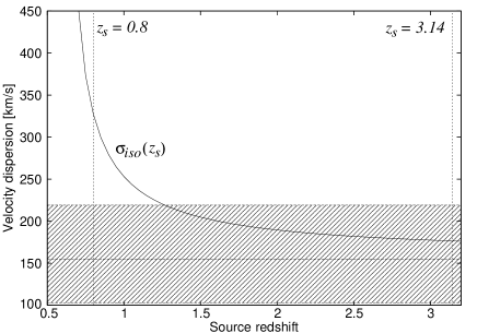
Figure 11: Velocity dispersion of L1 ($\sigma_{iso}$) as a function of source redshift ($z_{s}$), assuming an isothermal mass distribution in the lens. The shaded area represents the velocity dispersion derived from the fundamental plane at the 95% confidence level when $h=0.7$. Assuming an isothermal mass distribution, we find $z_{s}>1.2$ with 95% confidence.

The data available favour a high source redshift, but further spectroscopy will be essential if the radio source proves to be time-variable, since then B0631+519 would be a potential target for attempts to measure the Hubble constant. A spectroscopic source redshift would also be valuable for normalising mass models of this system.

4 Lens modelling of B0631+519

In this Section we seek to demonstrate that the lens hypothesis is a plausible explanation for the radio emission seen from B0631+519, by comparing the predictions of simple parametric mass models to the observations. We fit mass models to the 5 GHz MERLIN data on A1, A2, B1 and B2 because these images are relatively compact. We then take the optimum mass model fitted to the radio data and use it to invert the Einstein ring seen in the NICMOS F160W image by applying semi-linear inversion techniques (Warren & Dye, 2003; Treu & Koopmans, 2004; Koopmans, 2005). Finally, we use the mass model to examine L1’s mass to light ratio. The unknown source redshift means that the estimated time delays, as well as L1’s mass (within the Einstein radius) and its mass-to-light ratio are scaled by factors that depend on $z_{s}$ through combinations of the angular diameter distances between source, lens and observer. We therefore quote the affected quantities for $z_{s}=0.80$ and $z_{s}=3.14$.

4.1 Mass modelling using the 5 GHz MERLIN data

When fitting a mass model to the radio observations, the observed image positions are back-projected to the source plane through the current mass model. These back-projected images are used to update positions and flux densities of the model sources, and the updated sources are then projected forward onto the image plane and compared to the observed image positions and flux densities through a standard image-plane $\chi^{2}$ statistic (Kochanek, 1991). The statistic is defined over N images having angular positions $\mn@boldsymbol{\theta}_{i}$ ($i=1...N$) and flux densities $s_{i}$ by

$$\chi^{2}=\sum_{i=1}^{N}\frac{|{\mn@boldsymbol{\theta}_{i}-\mn@boldsymbol{\theta}_{i}^{\prime}}|^{2}}{{\sigma_{pi}}^{2}}+\sum_{i=1}^{N}\frac{|{s_{i}-s_{i}^{\prime}}|^{2}}{{\sigma_{fi}}^{2}},$$ (5)

where the primed quantities are values predicted by the lens model being evaluated and the $\sigma_{pi}$ and $\sigma_{fi}$ quantities account for errors in positions and flux densities respectively. The lens model parameters are iteratively optimised by a downhill simplex method (Press, Flannery & Teukolsky, 1986) until a minimum is found. In this approach we assume that the observed images are unresolved, which is clearly the case for A1 and B1 in the MERLIN 5 GHz data. A2 and B2 are slightly resolved but are still well-represented by Gaussian models. Components A1a, A1b, A1c and A1d will become useful if future high-resolution VLBI observations are able to resolve B1 into corresponding images. Without observed counterparts in B, the VLBA sub-components in A1 cannot yet be used to constrain the lens model. Images X, Y and Z are very extended and would be best treated using tools such as LensMEM (Wallington, Kochanek & Narayan, 1996) or LensClean (Kochanek & Narayan, 1992; Wucknitz, 2004).

Because A1 and B1 do not arise from the same source as A2 and B2, this system has fewer degrees of freedom immediately available than for a single quadruply imaged source. We ignore any contribution L2 might make to the lens effect and treat L1 as a singular isothermal ellipsoid (SIE; Kormann, Schneider & Bartelmann 1994). We allow the lens position to vary freely. The constraints available for this simple lens model are then four sets of image positions and flux densities. The free parameters are the positions and flux densities for two sources, the lens position, the lens mass scale and the position-angle and ellipticity of the mass distribution. The number of degrees of freedom, $\nu$, is therefore 1. We allow 20% errors on image flux densities to account for possible source variability, and we use the positions and position errors derived from the MERLIN 5 GHz data for A1, A2, B1 and B2 (because the VLBA observations resolve A2 and B2). The model parameters are shown in Table 8, and the lens is illustrated in Figure 12. The optimum model has a reduced $\chi^{2}$ of 0.41, with roughly equal contributions from flux densities and image positions.

Model	SIE	SIE$+$shear
Lens offset in R.A. [mas]	$+$398$\pm$23	$+$370 (fixed)
Lens offset in Dec. [mas]	$-$519$\pm$5	$-$520 (fixed)
Critical radius [mas]	603$\pm$2	605$\pm$3
Ellipticity	0.13$\pm$0.03	0.07$\pm$0.04
Lens P.A.	$-$57.1$\pm$0.1°	$-$28$\pm$12°
Shear strength		0.03$\pm$0.01
Shear P.A.		$-$81$\pm$0.5°
$\chi^{2}/\nu$	0.41/1	0.07/1

Table 8: Lens models for B0631+519. Lens position offsets are given with respect to image A1. Position angles are measured east of north. The errors in the lens parameters were estimated using Monte Carlo simulations.

Next, we fixed the galaxy position to that determined optically in Section 3, and added an external shear to the model. This SIE+shear model was then fitted to the MERLIN image positions and flux densities. The optimum model had a reduced $\chi^{2}$ of only 0.07 for 1 degree of freedom, suggesting that the random errors on the constraints were over-estimated. Reducing the flux density errors from 20% to 5% results in a reduced $\chi^{2}$ of 0.5 which is dominated by the contributions from the image positions. The optimum model parameters do not change significantly when the flux density errors are reduced. The optimum model parameters are listed in Table 8 and the model is illustrated in Figure 12. We note that the position of the best SIE-only lens is consistent with the optical lens position within the errors. The time delay between A1 and B1 is predicted to be 10.2 $h^{-1}$ days with the SIE model or 8.5 $h^{-1}$ days with the SIE+shear model for a source redshift of 3.14.

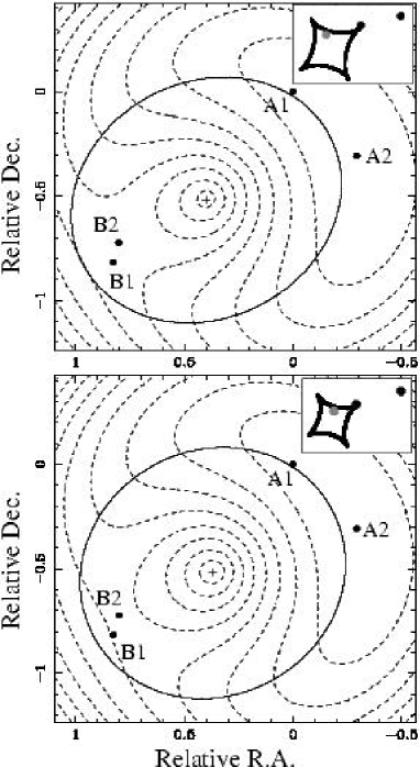
Figure 12: Lens models applied to B0631+519. The upper panel shows the best single SIE model. The lower panel shows the best SIE+shear model when the lens galaxy position is fixed to the measured optical/infrared galaxy position. The ellipse in each panel is the 4-image critical curve. The dashed contour lines represent the time delay surface of the lens relative to image A1. The contours in the upper panel begin at 1.23 $h^{-1}$ days (for the first contour surrounding A1/A2) and increase in steps of 2.05 $h^{-1}$ days. In the lower panel, the first contour surrounding A1/A2 represents 1.11 $h^{-1}$ days and the contours increase in steps of 1.88 $h^{-1}$ days. The contour levels are calculated for a source redshift of 3.14, and should be multiplied by a factor of 3.5 for $z_{s}=0.80$. The lensed images are represented by filled circles. The inset diagram shows the source plane; the astroid curve is the 4-image caustic, and filled circles represent the modelled source positions. The estimated position of the source responsible for images Y, Z and the arc X is marked by a light grey filled circle.

The lens modelling we have performed shows that the A1, A2, B1 and B2 components can be understood as lensed images of two distinct sources. It seems that A1 and B1 are images of a compact radio core having a flat (synchrotron self-absorbed) spectrum, while A2 and B2 arise from a more extended region of emission to the west of the core, probably a radio lobe. Images A1 and A2 have positive parity, while images B1 and B2 have negative parity. Incorporating images X, Y and Z is more difficult because they are all relatively extended compared to the A and B images, and the radio spectra indicate that these images arise from a third source. Back-projecting the positions of the Y and Z images (from the 1.7 GHz MERLIN data) to the source plane, along with the brightest point on arc X, produces an approximate source position of $+$0.41″east and $-$0.49″north relative to A1 (marked on Figure 12). The model thus suggests that the X, Y and Z images are produced by a counter-lobe on the eastern side of the source that happens to lie inside the 4-image caustic. With only the VLA data, showing X and Y but no Z, a model involving emission only on the western side of the source’s core might also be plausible.

4.2 Non-parametric de-lensing of the Einstein ring

The blue color of galaxy L2 and its consequent apparent absence in the HST-NICMOS F160W image, allows us to make use of the infrared Einstein ring to further test the validity of the lens mass model of CLASS 0631+519, which is based on the MERLIN radio data alone.

The Einstein ring is de-lensed (see Warren & Dye 2003; Treu & Koopmans 2004; Koopmans 2005), using the SIE plus shear model from Table 8. It is stressed that the lens mass model is not adjusted in any way to better fit the observed Einstein ring. A TinyTim generated PSF is used to account for blurring of the image. The structure of the Einstein ring is remarkably well reproduced (Figure 13), given that the lens mass model was only fitted to the radio jet structure. Despite the overall good quality of the reconstruction, a clear deviation from the model is found in the residual image, just north of L1 on the Einstein ring and slightly offset from the position of L2. Neither varying the mass model, nor alleviating the regularization can remove the feature completely.

We propose two possible explanations for this apparent “anomaly”: (a) it is due to residual emission from L2 – still present at a low level in the NICMOS-F160W image – or a dwarf-galaxy associated with L1, or (b) it is due to a small-scale perturbation of the lens mass model by the presence of L2, creating an anomaly in the ring (Koopmans, 2005) similar to flux-ratio anomalies in compact lensed sources (e.g. Mao & Schneider 1998). Although the first explanation(s) can not be completely excluded, the anomaly is situated near the brightness peak of the Einstein ring, appears to follow the curvature of the ring and is offset from the centroid of L2. Each of these observations seem to support the second explanation. As shown in Koopmans (2005), one would indeed expect such anomalies in Einstein rings, as a result of tiny perturbations of the dominant lens potential. The foreground galaxy L2 could provide the required perturbation. A full analysis of the nature of the anomaly, however, is beyond the scope of this paper.

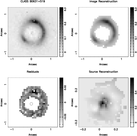
Figure 13: Non-parametric lens reconstruction of CLASS B0631+519. Top-left: The galaxy-subtracted NICMOS image of the Einstein ring. Top-right: The best reconstruction of the observed Einstein ring. Bottom-left: The residuals between observations and the model. Bottom-right: The reconstructed source brightness distribution. For the source reconstruction, we use a $30\times 30$ pixel grid with a scale of 0.02 arcsec pix^-1. We mask all image pixels below 3 $\sigma$ (indicated in the image reconstruction; $\sigma=0.011$ counts pix^-1). The regularization parameter for the source is $\lambda_{\rm s}=0.04$, resulting in $\chi^{2}/{\rm d.o.f.}\approx 1$. We use a regularization matrix that minimizes the curvature of the source (see Koopmans 2005). Note that a significant “anomaly” is left in the residual image (see text). The two circles in the residual image indicate the centroids of L1 (at the origin of the plot) and L2 at $-$0.33 arcsec east, $+$0.74 arcsec north of L1

4.3 Mass to light ratio of L1

We have sufficient information to estimate the B-band mass-to-light ratio of L1 in the region enclosed by the lensed images. The mass $M$ between the lensed images of a source (in the case of a circularly symmetric lens) is related to the image separation $\Delta\theta$ and the angular diameter distances $D_{l}$ (observer to lens), $D_{s}$ (observer to source) and $D_{ls}$ (lens to source) by

$$M=3.074\times 10^{7}~{}\frac{D_{l}D_{s}}{D_{ls}}~{}{\left(\Delta\theta\right)}^{2},$$ (6)

where $\Delta\theta$ is given in arcseconds. The estimate is significantly affected by the unknown source redshift (but not by assumptions concerning the distribution of mass inside the radius of the images). The ratio of angular diameter distances in Equation 6 decreases by a factor of $\sim$3.5 when the source redshift is increased from 0.8 to 3.14. We therefore estimate the lensing mass using both of the suggested redshifts for the source listed in McKean et al. (2004), since they conveniently span most of the range of plausible source redshifts. The separation between images A1 and B1 is 1.162$\pm$0.003 arcsec, which at the redshift of L1 corresponds to a linear distance of $5.6h^{-1}$ kpc. From Equation 6 we estimate the mass of L1 within the images at $2.17\pm 0.01\times 10^{11}h^{-1}$ $M_{\odot}$ using a source redshift of $z_{s}=0.80$ or $6.27\pm 0.03\times 10^{10}h^{-1}$ $M_{\odot}$ using $z_{s}=3.14$. Combining these estimates with the rest frame B-band absolute magnitudes derived from the Sérsic profile fits in Section 3.3 (corrected for a 1.16 arcsec diameter aperture) produces estimates for the mass-to-light ratio of L1 in the B filter of $15\pm 2h$ $M_{\odot}/L_{\odot}$ using $z_{s}=0.80$, or $4.3\pm 0.4h$ $M_{\odot}/L_{\odot}$ using $z_{s}=3.14$. We have taken the absolute magnitude of the Sun in B to be 5.54. The mass-to-light ratio estimates apply to the central region of L1 encircled by the lensed images (i.e. that within a mean radius of 2.8 $h^{-1}$ kpc from L1’s centre). Both figures are comparable with $M/L$ estimates from local ellipticals (Gerhard et al., 2001), although the figure for $z_{s}=3.14$ is relatively low given $h=0.7$.

5 Conclusions

Together the radio and optical/near-infrared observations presented here show that CLASS B0631+519 can be understood as a gravitational lens system. A simple SIE+shear mass model successfully reproduces features of the radio observations, and a non-parametric approach to the near-infrared data has identified the perturbing effect of L2 on the smooth lensing properties of the system. The mass modelling done so far leads us to conclude that the background radio source probably consists of three radio components in a classic double-lobed core-jet arrangement. The eastern lobe is located inside the quad-image caustic for the system and is lensed into the arc X and the more compact images Y and Z. The core region is doubly imaged into A1 and B1, while the western lobe is lensed into images A2 and B2. The magnification provided by the lens and the high resolution of the VLBA has allowed identification of the flat-spectrum AGN core and revealed jet components from both the approaching and the receding jets. The near-infrared source centre coincides with the radio source positions to within the errors.

The wealth of constraints available means that this system will benefit from application of deconvolution/inversion techniques that can utilise the extended images seen in the radio data. Having a good mass model for this system will allow us insights into the mass distributions of ellipticals at redshifts of 0.6, information that is not readily available in any other way. The hints of radio source variability mean that it may be possible to determine a radio time delay and use it to measure the Hubble constant.

This lens system is relatively unusual in having two galaxies of different redshifts present along the line of sight to the source, a situation that also occurs in CLASS B2114+022 (King et al., 1999; Augusto et al., 2001) and in PKS 1830-211 (Pramesh Rao & Subrahmanyan, 1988). In B2114+022 the effect of the nearer lens is much more significant than in B0631+519 (Chae, Mao & Augusto, 2001). In PKS 1830-211 the nearer lens was detected through its HI absorption (Lovell et al., 1996) at a redshift of 0.19 (the main lensing galaxy has a redshift of 0.886). The correct interpretation of the optical data in PKS 1830-211 is presently unclear, although the main lens is certainly a face-on spiral (Winn et al., 2002; Courbin et al., 2002).

Although L2 appears to have a relatively minor influence on the lensing properties of B0631+519, the radio emission from the lensed source must pass through L2’s ISM. Searches for molecular absorption lines may be worthwhile to provide extra information on the nature of this galaxy. The mass distribution in L2 may well be constrainable with further non-parametric modelling work.

References

- Augusto et al. (2001) Augusto P., et al., 2001, MNRAS, 326, 1007
- Bender et al. (1998) Bender R., Saglia R.P., Ziegler B., Belloni P., Greggio L., Hopp U., Bruzual G., 1998, ApJ, 493, 529
- Browne et al. (1998) Browne I.W.A., Wilkinson P.N., Patnaik A.R., Wrobel J.M., 1998, MNRAS, 293, 257
- Browne et al. (2003) Browne I.W.A., et al., 2003, MNRAS, 341, 13
- Bruzual & Charlot (1993) Bruzual A.G., Charlot S., 1993, ApJ, 405, 538
- Chae, Mao & Augusto (2001) Chae K.-H., Mao S., Augusto P., 2001, MNRAS, 326, 1015
- Condon et al. (1998) Condon J.J., Cotton W.D., Greisen E.W., Yin Q.F., Perley R.A., Taylor G.B., Broderick J.J., 1998, AJ, 115, 1693
- Courbin et al. (2002) Courbin F., Meylan G., Kneib J.P., Lidman C., 2002, ApJ, 575, 95
- da Silva Neto et al. (2005) da Silva Neto D.N., Andrei A.H., Assafin M., Vieira Martins R., 2005, A&A, 429, 739
- Djorgovski & Davis (1987) Djorgovski S.G., Davis M., 1987, ApJ, 313, 59
- Dressler et al. (1987) Dressler A., Lynden-Bell D., Burstein D., Davies R.J., Faber S.M., Terlevich R.J., Wegner G., 1987, ApJ, 313, 42
- Gerhard et al. (2001) Gerhard O., Kronawitter A., Saglia R.P., Bender R., 2001, AJ, 121, 1936
- Gregory et al. (1996) Gregory P.C., Scott W.K., Douglas K., Condon J.J., 1996, ApJS, 103, 427
- Högbom (1974) Högbom J.A., 1974, A&AS, 15, 417
- King et al. (1997) King L.J., Browne I.W.A., Muxlow T.W.B., Narasimha D., Patnaik A.R., Porcas R.W., Wilkinson P.N., 1997, MNRAS, 289, 450
- King et al. (1998) King L.J., et al., 1998, MNRAS, 295, L41
- King et al. (1999) King L.J., Browne I.W.A., Marlow D.R., Patnaik A.R., Wilkinson P.N., 1999, MNRAS, 307, 225
- Kinney et al. (1996) Kinney A.L., Calzetti D., Bohlin R.C., McQuade K., Storchi-Bergmann T., Schmitt H.R., 1996, ApJ, 467, 38
- Kochanek (1991) Kochanek C.S., 1991, ApJ, 373, 354
- Kochanek (1994) Kochanek C.S., 1994, ApJ, 436, 56
- Kochanek & Dalal (2004) Kochanek C.S., Dalal N., 2004, ApJ, 610, 69
- Kochanek & Narayan (1992) Kochanek C.S., Narayan R., 1992, ApJ, 401, 461
- Kochanek, Schneider & Wambsganss (2004) Kochanek C.S., Schneider P., Wambsganss J., 2004, Meylan G., Jetzer P., North P., eds, Gravitational Lensing: Strong, Weak & Micro, Proceedings of the 33rd Saas-Fee Advanced Course, Springer-Verlag: Berlin
- Koekemoer et al. (2002) Koekemoer A.M., Fruchter A.S., Hook R.N., Hack W., 2002, in Arriba S., ed, The 2002 HST Calibration Workshop: Hubble After the Installation of the ACS and the NICMOS Cooling System. Space Telescope Science Institute, Baltimore, MD, p. 339
- Koopmans (2005) Koopmans L.V.E., 2005, preprint (astro-ph/0501324)
- Koopmans & Treu (2003) Koopmans L.V.E., Treu T., 2003, ApJ, 583, 606
- Kormann, Schneider & Bartelmann (1994) Kormann R., Schneider P., Bartelmann M., 1994, A&A, 284, 285
- Krist (1993) Krist J., 1993, in Hanisch R.J., Brissenden R.J.V., Barnes J., eds, ASP Conf. Ser. Vol. 52, Astronomical Data Analysis Software and Systems II. Astron. Soc. Pac., San Francisco, p. 536
- Landolt (1992) Landolt A.U., 1992, AJ, 104, 340
- Lovell et al. (1996) Lovell J.E.J., et al., 1996, ApJ, 472, L5
- Mao & Schneider (1998) Mao S., Schneider P., 1998, MNRAS, 295, 587
- McKean et al. (2004) McKean J.P., Koopmans L.V.E., Browne I.W.A., Fassnacht C.D., Lubin L.M., Readhead A.C.S., 2004, MNRAS, 350, 167
- Myers et al. (2003) Myers S.T., et al., 2003, MNRAS, 341, 1
- Patnaik et al. (1992) Patnaik A.R., Browne I.W.A., Wilkinson P.N., Wrobel J.M., 1992, MNRAS, 254,655
- Pramesh Rao & Subrahmanyan (1988) Pramesh Rao A., Subrahmanyan R., 1988, MNRAS, 231, 229
- Press, Flannery & Teukolsky (1986) Press W.H., Flannery B.P., Teukolsky S.A., 1986, Numerical Recipes. Cambridge University Press
- Rengelink et al. (1997) Rengelink R., Tang Y., de Bruyn A.G., Miley G.K., Bremer M.N., Röttgering H.J.A., Bremer M.A.R., 1997, A&AS, 124, 259
- Rusin et al. (2002) Rusin D., Norbury M., Biggs A.D., Marlow D.R., Jackson N.J., Browne I.W.A., Wilkinson P.N., Myers S.T., 2002, MNRAS, 330, 205
- Rusin, Kochanek & Keeton (2003) Rusin D., Kochanek C.S., Keeton C.R., 2003, ApJ, 595, 29
- Rusin et al. (2003) Rusin D., et al., 2003, ApJ, 587, 143
- Rusin & Kochanek (2004) Rusin D., Kochanek C.S., 2004, preprint (astro-ph/0412001)
- Schlegel, Finkbeiner & Davis (1998) Schlegel D.J., Finkbeiner D.P., Davis M., 1998, ApJ, 500, 525
- Sérsic (1968) Sérsic J.L., 1968, Atlas de Galaxias Australes, Observatorie Astronómico de Córdoba, Argentina
- Shepherd (1997) Shepherd M.C., 1997, in Hunt G., Payne H.E., eds, ASP Conf. Ser. Vol. 125, Astronomical Data Analysis Software and Systems VI. Astron. Soc. Pac., San Francisco, p. 77
- Thomasson (1986) Thomasson P., 1986, QJRAS, 27, 413
- Tonry & Kochanek (2000) Tonry J.L., Kochanek C.S., 2000, AJ, 119, 1078
- Treu et al. (1999) Treu T., Stiavelli M., Casertano S., Møller P., Bertin G., 1999, MNRAS, 308, 1037
- Treu & Koopmans (2004) Treu T., Koopmans L.V.E., 2004, ApJ, 611, 739
- Wallington, Kochanek & Narayan (1996) Wallington S., Kochanek C.S., Narayan R., 1996, ApJ, 465, 64
- Warren & Dye (2003) Warren S.J., Dye S., 2003, ApJ, 590, 673
- Wilkinson et al. (1998) Wilkinson P.N., Browne I.W.A., Patnaik A.R., Wrobel J.M., Sorathia B., 1998, MNRAS, 300, 790
- Winn et al. (2002) Winn J.N., Kochanek C.S., McLeod B.A., Falco E.E., Impey C.D., Rix H.-W., 2002, ApJ, 575, 103
- Wucknitz (2004) Wucknitz O., 2004, MNRAS, 349, 1