The Spatial Orientation of Planetary Nebulae
Within the Milky Way

Abstract

We analyze the spatial orientation of a homogenous sample of 440 elongated Planetary Nebulae (PNe) in order to determine the orientation of their apparent major axis respect to the Milky Way plane. We present some important geometrical and statistical considerations that have been overlooked by the previous works on the subject. The global distribution of galactic position angles (GPA) of PNe is quantitatively not very different from a random distribution of orientations in the Galaxy. Nevertheless we find that there is at least one region on the sky, toward the galactic center, where a weak correlation may exist between the orientation of the major axis of some PNe and the Galactic equator, with an excess of axes with GPA$\sim 100^{\circ}$.

Therefore, we confirm that “extrinsic” phenomena (i.e., global galactic magnetic fields, shell compression from motion relative to the Interstellar Medium) do not determine the morphology of PNe on most of the sky, with a possible exception towards the galactic center.

1 INTRODUCTION

Since Charles Messier registered the first Planetary Nebulae (Dumbell Nebula in Vulpecula) on July 12, 1764 until the present time, over one thousand of these beautiful objects were found in our Galaxy and much more in nearby galaxies. It is well known that PNe have different shapes but, in most cases, the projection of a nebula onto the sky has a defined extension axis. Besides, the study of the orientation of many kind of phenomena such as supernova remnants (Gaensler 1998), orbits of binary systems (Brazhnikova et al. 1975), rotation of individual stars (Hensberge et al. 1979), has been of broad astrophysical interest. This sort of study provides information about formation, evolution and death of the stars.

However, the orientation of the projected major axis of the PNe was rarely studied and the results that were found are still contradictory.

For instance, Shain (1956) and Gurzadyan (1958) made the pioneering works about the orientation of PNe. They worked with very small samples from the Curtis catalogue (1917) and their conclusions were contradictory. Shain found that the angle between the semi-major axis of PNe and the galactic equator was small for objects with low latitudes. On the other hand Gurzadyan did not found any correlation and concluded that the magnetic field could not be influencing the shape of PNe. At the present time both papers only have a historical character. The first works to determine spatial orientations of PNe with a significant number of objects were those of Grinin & Zvereva (1968), and Melnick & Harwitt (1974). These works were more complete than early ones and both papers concluded that PNe are aligned with the plane. The hypothesis explaining these non-random orientations were based in the effect of the ambient magnetic field and interactions with the interstellar medium.

The works of Phillips (1997) and Corradi, Aznar & Mampaso (1998; hereafter CAM98) are the most recent and contradictory papers about global PNe orientations. In both cases, the images examined had high quality and the determination of PA have small errors, but they did not study the orientation of PNe over a specific region of the sky. The sample of Phillips was culled from a variety of published images complemented with broad band survey plates, whereas the sample of Corradi and coworkers comes mainly from three different narrow band surveys.

In this paper we visit this topic and make a careful study with new geometrical considerations. The characterization of any found correlation in a certain region of the sky would help to disentangle the role of the galactic magnetic field in determining the morphologies of these sources. Alternatively, it could be found that the motion of PNe through the interstellar medium leads to some compression of their shells, and result in significant correlations between the apparent outflow axes.

The unrestricted total sample was extracted from 3 different sources: Digitized Sky Survey version 2, DSS2 (red broad band); the Macquarie$/AAO/$Strasbourg $H_{\alpha}$ Planetary Nebulae Catalog, (MASH; $H_{\alpha}$ narrow band); and HST archival imagery (filters F502N and F656N). After the starting criteria described in Section 2, the initial number of PNe studied in this work resulted in 868, significantly larger than in previous studies. The analysis is performed through Sections 3 to 5, the results are presented and discussed in Sections 6 and 7.

2 SELECTION OF THE SAMPLE

The sample was extracted from the Catalogue of Galactic Planetary Nebulae updated version 2000 (Kohoutek 2001; hereafter CGPN2000) that includes 1510 true PNe and the MASH survey (Parker et al. 2006) with 903 objects, 578 of them are classified as true PN. There is virtually no overlap between the CGPN2000 and the MASH catalogs, therefore this last one provided one third of the final sample of truly elongated PNe. We included a special subsample of the CGPN2000 which is formed by those objects imaged by the Hubble Space Telescope (HST).

The selection criteria employed to obtain our final sample were:

1. Objects classified as true PN.

2. Angular size larger than 10$\arcsec$. The experience shows that, in general, this limit yields spatial resolution sufficient to determine the orientation of the major axis. Exception in the angular size criterium was made for those objects imaged by the HST.

3. $b<20^{\circ}$, to avoid information degradation by projection effects over high latitudes objects.

4. In case of the MASH survey we only included PNe which at least have one confirmation spectrum.

5. Objects clearly visible in the DSS2 plates (surface brightness $<$ 17 mag/arcmin²), this restriction criterium was applied for all the surveys contributing to the sample.

6. Elongated shape (PNe with morphology type R were rejected).

By elongated shape PNe we mean bipolar nebulae or those which show two lobes defining unambiguously the direction of their polar outflows, as well as E nebulae with an appreciable ellipticity. At the cases where the object is near to the DSS resolution we estimate an empirical limit of major to minor axis length ratio 1.2:1, as determined from those objects which were in the visual limit of acceptance.

In order to extend our sample we included PNe with angular size between 4$\arcsec$ and 10$\arcsec$ inclusively, that had been observed by HST. Such PNe, 42 in total number and 27 truly elongated, belong to some of our 4 regions. Due to the variety of filters the chosen criterium here was to use the images taken through the F656N or F502N filters whenever possible. To complete the sample we also included those PNe measured by CAM98 that we could not measure from the DSS2 plates. After a careful examination of more than 868 PNe in the initial list (obtained after criteria 1, 2 and 3), we arrived to the final sample that contains 444 truly elongated PNe distributed in four regions, 174 belonging to the MASH sample. The remaining objects were planetaries with apparent circular shape, low surface brightness or very peculiar morphology.

3 MEASUREMENT OF POSITION ANGLES

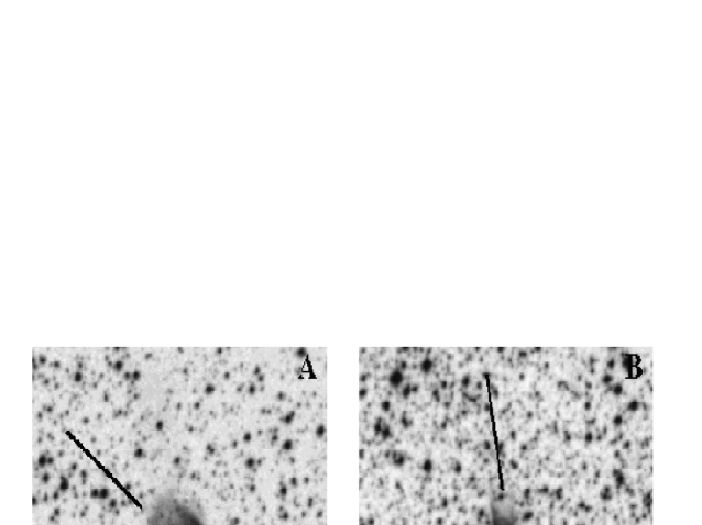
Figure 1: Examples of the applied measuring criteria. The objects are: A) NGC 4071, B) Mz3, C) NGC 5189 and D) NGC 650. All the images belong to the DSS, red band. North is up and East to the left.

We measured the position angles (PA) of the projected major axis over the sky, for all the PNe of the final sample. PA are measured following the usual convention: from the north towards the east. These angles are measured within the equatorial coordinates system so we call them EPA. The directions of the elongated axis were estimated visually by fixing the line that better represents the long symmetry axis of the PN. The angle that this line forms with the north was the EPA. For bipolar structures the EPA was measured with respect to the direction of the outflow of the objects. The uncertainties of EPA are estimated following the criterium of CAM98: all measurements were repeated independently by both authors. The largest difference between both measurements was 8^∘. The measuring criteria are exemplified in Fig. 1.

In spite of the fact that all previous works determined the EPA visually, we tried to obtain those angles through an automated way, but the problem was that this sort of automated algorithms are still not powerful enough to deal with low S/N and overcrowded fields with high galactic background. PNe are usually located in highly populated Milky Way fields and in many cases do not show structure complete at the same surface brightness. This patchy structure and the star images make the software approach still difficult.

An example of a more refined criterion of EPA measurement can be derived from an attentive comparison between the Fig. 1c and 1d. In spite of the fact that both objects present the characteristic belt of bipolar planetary nebulae, in the case of NGC 5189 the structures that appear in both sides of the apparent belt do not have hemispherical appearance as the case shown in Fig. 1d. The orientation marked in the figure takes into account that the brilliant knot at the E of the main body’s external part, is of totally nebular appearance when the original image is inspected. Considering that the criterion for determination is based mainly on the external morphology, the major axis of the PN is well determined. This complex object represents a limit case where the measured EPA could show the largest scatter when employing other criteria. But as we show in Section 7, our EPA values do not show significant deviations from the values obtained by CAM98 for objects present in both samples.

4 TRANSFORMATION TO THE GALACTIC SYSTEM

The EPAs are measured relative to the equatorial coordinates system. In order to transform this position angle to the galactic system we need to compute the angle $\beta$, which is subtended at the position of each object by the direction of the equatorial north and the galactic north.

$$\sin\beta=\frac{\cos\delta_{0}\sin(\alpha_{0}-\alpha)}{\cos b}$$

Where $\delta_{0}$ and $\alpha_{0}$ are the equatorial coordinates of the galactic North Pole, $\alpha$ and $b$ are the equatorial right ascension and galactic latitude coordinates respectively (both coordinates were extracted from CGPN2000). Then the galactic position angle (GPA) is defined as the position angle of the major axis of the apparent nebular elongation, measured from the direction of the galactic north towards the east (Table 4).

$$GPA=EPA-\beta$$

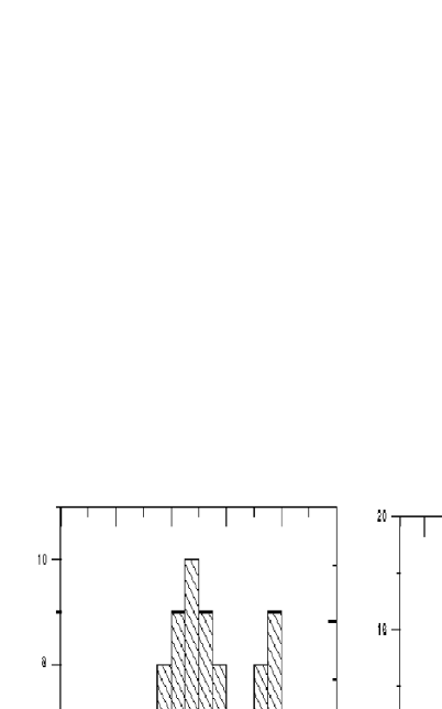
Figure 2: Test distribution of position angles, simulating two peaks not very near to the Galactic plane with PA computed in the interval $[0^{\circ},180^{\circ}]$ (left), and the corresponding inferred distribution if the values are reported as some authors have done, in the interval $[0^{\circ},90^{\circ}]$ (right).

We used the same convention that Phillips (1997) used for measuring the EPAs, in the interval $[0^{\circ},180^{\circ}]$. The values are reported and used here in the same range, but some authors (e.g. CAM98) report them to the interval $[0^{\circ},90^{\circ}]$ assuming a priori a symmetric problem, in the sense that a preferred orientation of the PNe elongations very nearly to the galactic equator will be easier to detect. The problem with this treatment of the EPA is that it would blur any other preferred orientation that is not very near to the galactic equator (Fig. 2).

5 STUDIED REGIONS

The orientations for individual planetary nebulae is presented in Table 4, which is also available on request to the authors. One difference with previous studies is that, in order to avoid information degradation by projection effects, we did not include in our study objects with $\mid b\mid>20^{\circ}$. The number of objects far from the galactic plane is not statistically significant, although the projection effect with respect to the galactic equatorial plane should be considered in any future larger sample to be analyzed. To study the orientation of the sample, we selected four angular sectors: those defined by the galactic center and anti-center, and the perpendicular directions (Table 1).

The regions were defined in angular range in such a way that there was enough number of objects to do a statistical analysis in at least the region towards the galactic center (262 objects). But they should not be so large in angular extent that any absolute orientation respect to the galactic system would be deleted by the superposition of different projections to the observer. It must be taken into account, that the projection effects at the position of the observer would mask the effect of some preferred orientations if the data are compiled and analyzed as a whole set without any regard to the position respect to the observer and the galactic center. All the previous works have treated the data as a whole set, and we show that in this way important information could have been or might be overlooked in the future.

6 RESULTS

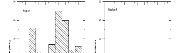
Figure 3: Distribution of GPA of the regions presented in Table 1.

The region that shows a distribution of GPA with some possible non-random characteristics is the region with center towards the galactic center. In the other regions, the low number of objects precludes detection of any clear trend, although we can rule out any strong correlation that involves the majority of the PNe in the sample. The distribution of GPA of the regions are presented in Fig. 3.

If the distribution of the N objects of the sample in each sector were random, with the same probability of finding an elongated object with its axis towards any PA, when j angular boxes are defined in the range $[0^{\circ},180^{\circ}]$, it could be expected an average population of N/j objects per bin. The frequency of all the possible values would be an angular positions distribution, with a dispersion $\mathbf{\sigma=(N/j)^{1/2}}$. In Table 2 we show the expected average per angular bin and the dispersion for each region, and the number of peaks observed above $2\mathbf{\sigma}$ and $1\mathbf{\sigma}$.

The barycenters calculated for each peak, determined within a window of $60^{\circ}$, are summarized in Table 2. A thorough test can be performed by applying a simple binomial test, as proposed by Siegel (1956) and applied by Hutsemékers (1998). It gives the probability $P_{s}$ that a random distribution has $L_{s}$ angles (of a set of $N$ objects) in the interval $[P_{m}-\alpha,P_{m}+\alpha]$. In our case $P_{m}$ is the peak barycenter. Such probability is defined as:

$$P_{s}=\sum_{l=l_{s}}^{N}\left(\frac{\alpha}{90}\right)^{l}\left(1-\frac{\alpha}{90}\right)^{N-l}{N\choose l}$$

Table 3 shows the probability of randomness for each observed peak using $\alpha=20^{\circ}$ and $\alpha=10^{\circ}$ (note that when $\alpha=20^{\circ}$ the probability that the right peak of region I is random, is only $P=0.016$). In region I, the distribution has two peaks with a separation of $\sim 80^{\circ}$ (or $\sim 100^{\circ}$ in the opposite sense) in the directions defined by the peaks. It is important to remark that the separate subsamples of PNe from DSS2, CAM98 and MASH each one shows at the region I, an apparent peak in $GPA\simeq 100^{\circ}$.

Following the clue provided by some similarity of the results for regions III and IV, we added the distributions found for regions I and II (Fig. 4a) and for regions III and IV (Fig. 4b). The two distributions in Fig. 4b show right peak over $2\sigma$ and left peak over $1\sigma$, in both cases with a peak separation of $80^{\circ}$. Here the separation is considered as the minimum angular distance between both peaks. Moreover as both distributions are in opposite sides of the sky, is natural to measure the separation in opposite sense. It should be noted that the position angles are being measured with the NESW convention, without any regard to the absolute orientation of the objects respect to the observer. Then if some absolute orientation would be common to most of the objects and considering that the observer is in the center of the sky band over which the objects appear projected, the sense of measuring of the position angles in opposite regions (e.g. I and II) should be inverted by making 180 - GPA in the opposite regions. Coincidentally, the transformation of the data in regions III+IV (Fig. 4b) gives a distribution resembling that of regions I+II: a narrow main peak and a possible secondary one $80^{\circ}$ before.

We also carried out the Kolmogorov-Smirnov (K-S) test to have an alternative evaluation of the randomness of the observed distribution. This requires the calculation of $D_{max}$: the absolute value of the maximum deviation between the observed ($S_{N}(x)$ with $N_{1}$ points) and theoretical ($P(x)$ with $N_{2}$ points) cumulative distribution function (Press et al. 1992). The significance can be written as the following sum:

$$Q_{ks}=2\sum_{j=1}^{\infty}(-1)^{(j-1)}e^{-2j^{2}\lambda^{2}}$$

Where $\lambda=(\sqrt{N_{e}}+0.12+0.11/\sqrt{N_{e}})D_{max}$ and $N_{e}=N_{1}N_{2}/(N_{1}+N_{2})$ that is the effective number of data points of the samples. This test gave us a probability, that our data derived from a random distribution, of 63% for region I, 53% for region II, 93% for region III and 28% for region IV.

As an alternative we tried to perform a variation of K-S test: the Kuiper (K-P) test which is more sensible than K-S test in some kind of circular distributions.

To perform this test we have to calculate $V=D_{+}+D_{-}$, which is the sum of the maximum distance of $S_{N}(x)$ above and below $P(x)$. A good approximation for the significance is:

$$Q_{kp}=2\sum_{j=1}^{\infty}(4j^{2}\lambda^{2}-1)e^{-2j^{2}\lambda^{2}}$$

Where $\lambda=(\sqrt{N_{e}}+0.155+0.24/\sqrt{N_{e}})V$

The result that we obtained with K-P test for our region I (with the strongest signal) is $Q_{KP}=35\%$, which seems to be not a convincing one. These tests could not be fully applicable to our kind of data: caution should be taken when applying all varieties of K-S test, because they lack the ability to discriminate some kind of distributions. For example, we can consider a probability distribution showing a narrow hole within which the randomness probability falls to zero. The existence of even one data point within the hole would rule out such distribution (because of its cumulative nature, Press et al. 1992), the K-S test would require many data points in the narrow hole before signaling a discrepancy.

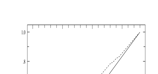
Figure 6: K-P test comparison percentile plot of the distribution shown in (Fig.6). Despite the clear 3 sigma signal presented, the largest $D_{max}$ yields, through the K-P test, a probability of $67\%$.

To probe this kind of behavior, we generated a random distribution of 72 GPA and after that we added 10 GPA values distributed in the first bin (Fig. 5). This distribution has an average of 9.1 GPA per bin and a dispersion of $\sigma=3.0$. In this way, the first bin shows a signal over $3\sigma$. Now if we apply both tests to this artificial sample we obtain the next probabilities, that this data follow a random distribution: $Q_{KS}=17\%$ and $Q_{KP}=67\%$ (Fig. 6). We have verified that there is no way to generate 67 cases and not even 17 cases of a $3\sigma$ peak in 100 fully random samples.

Therefore we conclude that although K-S and K-P tests are well suited to analyze non random global trends in samples, they are strongly insensitive to the presence of a local non-random feature.

7 DISCUSSION

We studied the orientation of all PNe of our sample (without separating it in regions) and we do not see a clear preferential orientation of long axis of PN respect to the galactic plane. This distribution of GPA is similar to that observed by CAM98. We tried to double check our results by applying our analysis to the data published by CAM98, performing a suitable analysis to take over the ambiguity of the position angles (assigned to the range $[0^{\circ},90^{\circ}]$). More precisely, the sample of CAM98 includes 208 objects (counting the object M2-55 in only one list); 69 of them are in both samples (the object that CAM98 put in the list of ellipticals as PC 4, is in fact PB 4); 85 are outside our four regions; 50 were not measured because they are too small; have strange morphology or circular appearance; and 4 objects are not true PN (Bl Cru, CRL 2688, M 1-91, M 1-92). 75$\%$ of the 69 objects that are in both samples, have their GPA in good agreement ($\pm 10^{\circ}$) with our measurement. Moreover, the distribution of GPA from those objects from CAM98 whose coordinates are in region I, shows a clear peak over 3 $\sigma$ (Fig. 7, 48 objects), whose barycenter is in $100^{\circ}\pm 15^{\circ}$, a position similar, within the uncertainties, to the main peak in our Fig. 3. This feature could not be detected by CAM98 due to the way they calculated the final angles to plot. The differences could be mainly caused by the fact that they employed deep narrow-band images, as shown in Fig. 8. This figure shows an example of the PN TH2-A DSS image through R broad-band filter and 1.5″  resolution. The EPA was measured following the ellipsoid apparent major axis. For comparison, Fig. 8-right shows the same object imaged with GMOS at Gemini-S 8 m telescope, through a [OIII]$\lambda$5007 filter and with 0.7″  seeing (from Díaz et al., in preparation). The presence of faint blue emission knots can change the major axis determination from the ellipsoid maximum diameter to an approximately perpendicular angle. Therefore it can be expected that the measured geometrical properties of the objects change as distinct ionization layers are imaged through different filters, more precisely, the left peak (e.g. We 1-4) in our broad band study could be arose in the measuring of the PN equatorial belt apparent axis instead of the faint external envelope. This should not occur in the deep narrow band images of the CAM98 sample and could explain the absence of the second peak in that sample. Nevertheless, the agreement between the GPA measurements in both samples is very good and the presence of the second peak can just be ascribed to the ability to detect the outer fainter details in the deep narrow band images, which are usually perpendicular to the bright equatorial belt structures more easily detected in the DSS imagery.

An interesting test to perform is to check if the distribution of GPA in the four regions has a distance modulation and consider objects statistically far and close. As a first order approach we separated objects in each region by its angular size: an angular diameter of 35$\arcsec$ divided the sample in two halves, objects with large angular size were considered closer than the ones with small angular size. Assuming an average radius of 0.1 pc the separating distance is 1.2 kpc. The results that we obtained in the four regions show that the distribution of GPA for larger PNe has the same shape than the smaller PNe. So there is not evidence about a distance effect.

Following the same open minded search we tried to relate the PA of the long axis of PNe with respect to the Gould Belt, the plane defined by nearby stars of young population, mainly O and B stars (Cameron et al. 1994). The result found shows a noisy distribution of PA. Besides, several studies have related bipolar PNe with binary progenitors (Bond & Livio 1990) but the antecedents about the orientations of the orbits of binary stars do not provide any comparable result. Notwithstanding it must be remarked that a thorough analysis should be made, keeping in mind the new geometric considerations carried out in this work.

We could also consider the case in which only the disk population of the PNe towards the galactic center would show a preferred orientation. First, we can test the robustness of the result against the possibility of significant contamination of the PNe sample toward the galactic center caused by a random orientation of bulge PNe. If the bulge PNe contamination were as high as 50%, then more than half of the disk PNe would need to have a preferred orientation near to the galactic plane, to be detected and identified in the EPA distribution. Moreover, it would be necessary to disentangle the bulge objects by their radial velocities in order to verify if the preferred orientation for the disk PNe is actually much larger than the one reported here.

Regarding the physical causes, Melnick & Harwitt (1974) mentioned the compression of the PNe shells resulting from motion through the ISM is seldom observed, remarking that the time scale of the PN expansion ($10^{4}$ years) would be large enough to show systematic off-centering of the progenitor stars, which heretofore has been detected in a few lopsided objects (Borkowski, Sarazin & Soker 1990) and could be a dominant factor at the very faintest outer envelopes where the nebular density falls below a critical limit of N${}_{H}\sim 40$ cm^-3. Undoubtedly the most considered hypothesis has been that the PNe could eventually expand more in the direction of the ambient or galactic magnetic field field force lines, which are approximately deployed along the Milky Way plane (e.g. Phillips 1997). The typical energy density of the interstellar magnetic field is lower than $B^{2}/8\Pi\approx 1.5E-11$ erg cm^-3, whereas the energy density (thermal, excitation and ionization) is usually larger than $E-9$ erg cm^-3, consequently a correlation with any observable quantity related with galactic magnetic fields (Diaz & Weidmann 2008, in preparation) would imply that this are at least one or two orders of magnitude higher in some regions towards the galactic center.

8 FINAL REMARKS

The data on PA of planetary nebulae show that global preferred orientations are not dominant, even considering a new approach that takes into account the three-dimensional problem. Besides the conclusions hold by the results, we presented here some important geometrical and analytical considerations that have been overlooked by the previous works on the subject.

It is worth to mention that there could be a preferred orientation of some PNe in the zones near to the galactic center, and the corresponding distribution of galactic position angles could have a peak not exactly aligned with the Milky Way plane: the PNe towards the galactic center have an orientation distribution with a possible narrow peak near to the galactic plane ($GPA\simeq 100^{\circ}$), with a randomness probability as small as $0.01$. We remark that we did not exclude any object within the selection criteria and galactic coordinates in the range $-30<l<30$ and $-20<b<20$, and no special attention was given to the possibility that some objects may belong to the galactic bulge population and the consequences over the detected trend are unknown beyond the qualitative discussion of the previous section.

Furthermore a larger and deeper galactic center sample, optimally observed at NIR wavelengths, should be analyzed in order to thoroughly assess the reality of this preferred orientation. The possible implications are of broad astrophysical interest and we hope that they stimulate more detailed studies, in particular, larger samples of galactic PNe towards the galactic center should be studied as soon as they become available.

Table 1: Sampled galactic sectors.

Sector	l range [∘]	b range [∘]	Number of objects
Galactic center (Region I)	-30 a 30	-20 a 20	262
Local motion apex (Region II)	60 a 120	-20 a 20	71
Galactic anti-center (Region III)	150 a 210	-20 a 20	21
Local motion antapex (Region IV)	240 a 300	-20 a 20	90

Table 2: GPA Barycenters of the peaks observed in Fig. 3, in degrees.

Region	Expected Average	Dispersion	$2\sigma$ peak?	Baryc.1	Baryc.2	Separation
	(number per bin)			(main peak)
I	29.1	5.4	yes	20 $\pm$ 16	101 $\pm$ 16	81
II	7.9	2.8	-	6 $\pm$ 17	-	-
III	2.3	1.5	-	79 $\pm$ 15	158 $\pm$ 16	79
IV	10.0	3.2	yes	84 $\pm$ 15	158 $\pm$ 16	74

Table 3: Randomness probabilities of each sector with a peak width of $20^{\circ}(\alpha=10^{\circ})$ and $40^{\circ}(\alpha=20^{\circ})$.

Regions	(Left peak)20	(Right peak)20	(Left peak)10	(Right peak)10
I	0.841	0.003	0.077	0.0004
II	0.215	-	0.091	-
III	0.317	0.317	0.199	0.418
IV	0.003	0.732	0.020	0.039

Table 4: PN Data.

Name	l [∘]	b [∘]	EPA [∘]	GPA[∘]	Source
G000.0-01.8	0	-1.8	163	42	MASH
M 2-19	0.2	-1.9	110	170	CAM98
G000.2-03.4	0.2	-3.4	100	160	MASH
IC 4634	0.3	12.2	153	27	DSS2
G000.3+07.3	0.3	7.3	90	145	MASH
G000.3+04.5	0.3	4.5	160	36	MASH
K 1-4	1	1.9	155	33	DSS2
G001.2-05.6	1.2	-5.6	138	19	MASH
He 2-262	1.3	2.2	21	78	HST
G001.5-02.4	1.5	-2.4	60	120	MASH
SwSt 1	1.6	-6.7	126	8	HST
H 1-55	1.7	-4.5	90	151	HST
G001.8-05.0	1.8	-5	55	116	MASH
G001.9+02.1	1.9	2.1	80	138	MASH
IC 4776	2	-13.4	34	100	CAM98
G002.0+06.6	2	6.6	60	116	MASH
G002.0+01.5	2	1.5	115	173	MASH
G002.0-03.2	2	-3.2	95	155	MASH
G002.1-02.4	2.1	-2.4	130	10	MASH
G002.1-02.8	2.1	-2.8	15	75	MASH
H 1-54	2.1	-4.2	137	18	HST
G002.2+05.8	2.2	5.8	5	61	MASH
G002.2-01.2	2.2	-1.2	40	99	MASH
G002.3+01.7	2.3	1.7	35	93	MASH
Cn 1-5	2.3	-9.5	162	45	HST
NGC 6369	2.4	5.9	135	44	DSS2
G002.4+03.5	2.4	3.5	46	103	MASH
G002.4+01.1	2.4	1.1	62	120	MASH
G002.4-05.0	2.4	-5	15	76	MASH
H 2-37	2.4	-3.4	71	131	HST
G002.5+04.8	2.5	4.8	16	73	MASH
M 1-42	2.7	-4.8	21	83	CAM98
G002.8-04.1	2.8	-4.1	65	126	MASH
Te 1567	2.8	1.8	0	58	HST
G002.9-03.0	2.9	-3	15	75	MASH
G003.0-01.7	3	-1.7	140	20	MASH
G003.1+05.2	3.1	5.2	135	12	MASH
G003.1-01.6	3.1	-1.6	100	160	MASH
Hb 4	3.2	2.9	140	18	HST
G003.3-01.6	3.3	-1.6	30	90	MASH
IC 4673	3.5	-2.4	126	7	DSS2
G003.5+04.5	3.5	4.5	35	92	MASH
G003.5+02.6	3.5	2.6	45	103	MASH
G003.6-03.0	3.6	-3	145	25	MASH
H 2-15	3.8	5.3	R	…	HST
H 1-59	3.9	-4.4	71	132	HST
G004.0-02.6	4	-2.6	115	175	MASH
G004.0-02.7	4	-2.7	92	152	MASH
G004.1-03.3	4.1	-3.3	85	145	MASH
G004.2-02.5	4.2	-2.5	140	20	MASH
G004.5+06.0	4.5	6	60	117	MASH
H 2-12	4.5	6.8	…	…	HST
G004.8-01.1	4.8	-1.1	32	92	MASH
H 2-25	4.9	2.1	41	99	HST
M 1-25	4.9	4.9	40	97	HST
G005.0+02.2	5	2.2	166	44	MASH
G005.4-03.4	5.4	-3.4	168	49	MASH
G005.9-09.8	5.9	-9.8	140	24	MASH
M 1-28	6	3.1	14	73	DSS2
G006.1+03.8	6.1	3.8	0	58	MASH
G006.1+01.5	6.1	1.5	65	124	MASH
M 1-20	6.2	8.4	102	159	HST
G006.3+01.7	6.3	1.7	170	49	MASH
G006.4-03.4	6.4	-3.4	147	28	MASH
G006.4-05.5	6.4	-5.5	140	22	MASH
G006.5+08.7	6.5	8.7	54	111	MASH
G006.5-03.9	6.5	-3.9	20	81	MASH
M 3-15	6.8	4.2	122	0	HST
G007.1+07.3	7.1	7.3	136	13	MASH
G007.1+04.9	7.1	4.9	118	176	MASH
G007.1-05.0	7.1	-5	65	127	MASH
G007.3+01.7	7.3	1.7	30	89	MASH
G007.4+01.7	7.4	1.7	13	72	MASH
M 2-34	7.8	-3.7	177	59	DSS2
G007.8+04.3	7.8	4.3	80	138	MASH
H 1-65	7.9	-4.4	R	…	HST
NGC 6445	8	3.9	149	110	DSS2
M 1-40	8.3	-1.1	44	105	CAM98
G008.3+09.6	8.3	9.6	120	177	MASH
He 2-260	8.3	6.9	85	143	HST
G008.4-02.8	8.4	-2.8	85	146	MASH
G008.7-04.2	8.7	-4.2	135	17	MASH
G009.0-02.2	9	-2.2	15	76	MASH
G009.0-02.4	9	-2.4	18	79	MASH
G009.4-01.2	9.4	-1.2	53	114	MASH
NGC 6309	9.6	14.8	56	114	DSS2
A 41	9.6	10.5	143	21	DSS2
G009.8-01.1	9.8	-1.1	10	71	MASH
G009.9+04.5	9.9	4.5	60	119	MASH
G010.0-01.5	10	-1.5	65	126	MASH
NGC 6537	10.1	0.7	38	99	DSS2
G010.2+00.3	10.2	0.3	50	110	MASH
M 2-9	10.8	18.1	179	57	DSS2
IC 4732	10.8	-6.5	R	…	HST
NGC 6578	10.8	-1.8	144	25	HST
G011.0+01.4	11	1.4	60	120	MASH
M 2-13	11.1	11.5	40	98	CAM98
DeHt 10	11.4	17.9	175	53	DSS2
NGC 6567	11.8	-0.7	107	168	HST
G011.9+07.3	11.9	7.3	165	44	MASH
G012.1+02.8	12.1	2.8	150	30	MASH
PM 1-188	12.2	4.9	R	…	HST
G012.5+04.3	12.5	4.3	113	173	MASH
G013.1+05.0	13.1	5	85	145	MASH
M 1-33	13.1	4.2	30	90	HST
G013.6-04.6	13.6	-4.6	90	152	MASH
We 4-5	13.7	-15.3	141	27	DSS2
SaWe 3	13.8	-2.8	133	15	DSS2
G014.6+02.3	14.6	2.3	50	110	MASH
G014.6+01.0	14.6	1	175	56	MASH
A 44	15.6	-3	131	13	DSS2
M 1-39	15.9	3.4	80	140	HST
M 1-54	16	-4.3	104	167	DSS2
G016.0-07.6	16	-7.6	135	18	MASH
G016.3-02.3	16.3	-2.3	168	50	MASH
G016.4-00.9	16.4	-0.9	139	20	MASH
G016.6+03.1	16.6	3.1	90	151	MASH
G018.0-02.2	18	-2.2	56	118	MASH
G018.5-01.6	18.5	-1.6	160	42	MASH
DeHt 3	19.4	-13.6	13	73	DSS2
CTS 1	19.8	5.6	102	163	CAM98
G020.4+02.2	20.4	2.2	115	176	MASH
M 1-51	20.9	-1.1	29	92	CAM98
M 3-55	21.7	-0.6	57	120	CAM98
M 3-28	21.8	-0.5	2	64	DSS2
M 1-57	22.1	-2.4	137	20	CAM98
M 1-58	22.1	-3.2	78	140	HST
MaC 1-13	22.5	1	26	88	DSS2
G023.4+00.7	23.4	0.7	145	27	MASH
M 1-59	23.9	-2.3	116	179	CAM98
M 2-40	24.1	3.8	80	142	CAM98
M 4-9	24.2	5.9	167	50	DSS2
Pe 1-17	24.3	-3.3	45	108	CAM98
G024.4-03.5	24.4	-3.5	60	122	MASH
A 60	25	-11.7	103	166	DSS2
IC 1295	25.4	-4.7	69	132	CAM98
NGC 6818	25.8	-17.9	13	79	CAM98
Pe 1-14	25.9	-0.9	45	108	CAM98
G026.2-03.4	26.2	-3.4	7	69	MASH
G026.4+02.7	26.4	2.7	25	87	MASH
G026.9-00.7	26.9	-0.7	56	118	MASH
A 49	27.3	-3.4	31	94	CAM98
DeHt 2	27.6	16.9	44	107	DSS2
G027.6-00.8	27.6	-0.8	40	102	MASH
G027.8+02.7	27.8	2.7	50	112	MASH
WeSb 3	28	10.3	145	31	DSS2
Pe 1-20	28.2	-4	12	75	CAM98
K 3-2	28.6	5.2	…	…	HST
G028.7-03.2	28.7	-3.2	40	102	MASH
A 48	29	0.5	37	99	DSS2
NGC 6751	29.2	-5.9	81	144	DSS2
G029.8+00.5	29.8	0.5	20	82	MASH
A 68	60	-4.3	13	72	CAM98
NGC 6886	60.1	-7.7	54	111	CAM98
K 3-45	60.5	-0.3	18	78	CAM98
NGC 6853	60.8	-3.7	129	6	DSS2
He 2-437	61.3	3.6	77	138	DSS2
M 1-91	61.4	3.6	77	138	CAM98
NGC 6905	61.4	-9.6	161	36	DSS2
M 2-48	62.4	-0.3	67	125	DSS2
NGC 6720	63.1	14	57	123	DSS2
M 1-92	64.1	4.3	130	11	CAM98
BD+30 3639	64.8	5	R	…	HST
We 1-9	65.1	-3.5	70	126	DSS2
He 1-6	65.2	-5.7	122	177	DSS2
He 2-459	68.4	-2.7	57	113	HST
M 1-75	68.8	0	152	28	DSS2
K 3-46	69.2	3.8	110	168	DSS2
NGC 6894	69.4	-2.6	145	20	DSS2
K 3-58	69.6	-3.9	83	137	DSS2
M 3-35	71.6	-2.3	48	103	CAM98
K 3-57	72.1	0.1	33	90	CAM98
A 74	72.7	-17.1	52	99	DSS2
K 3-76	73	-2.4	134	9	CAM98
GM 1-11	73	-2.2	65	119	DSS2
NGC 6881	74.5	2.1	139	16	CAM98
Anon	75.6	4.3	109	166	DSS2
A 69	76.3	1.2	54	108	DSS2
Dd 1	78.6	5.2	81	137	DSS2
M 4-17	79.6	5.8	118	174	DSS2
CRL 2688	80.1	-6.5	14	63	CAM98
A 78	81.2	-14.9	146	9	DSS2
NGC 6884	82.1	7.1	174	51	HST
K 4-55	84.2	1	85	135	DSS2
A 71	84.9	4.4	15	68	DSS2
Hu 1-2	86.5	-8.8	129	172	CAM98
We 2-245	87.4	-3.8	137	1	DSS2
NGC 7048	88.7	-1.6	15	60	DSS2
NGC 7026	89	0.3	4	51	DSS2
Sh 1-89	89.8	-0.6	50	95	DSS2
K 3-84	91.6	-4.8	3	45	CAM98
We 1-11	91.6	1.8	49	95	DSS2
K 3-79	92.1	5.8	132	1	DSS2
M 1-79	93.3	-2.4	88	129	DSS2
NGC 7008	93.4	5.4	38	86	DSS2
K 3-83	94.5	-0.8	100	142	CAM98
A 73	95.2	7.8	38	87	DSS2
K 3-61	96.3	2.3	164	27	CAM98
M 2-50	97.6	-2.4	52	90	CAM98
Me 2-2	100	-8.8	R	…	HST
IC 5217	100.6	-5.4	90	122	CAM98
A 75	101.8	8.7	94	137	DSS2
A 80	102.8	-5	19	48	DSS2
A 79	102.9	-2.3	20	51	DSS2
M 2-51	103.2	0.6	151	4	DSS2
M 2-52	103.7	0.4	116	148	DSS2
KLW 8	104.1	-1.4	40	70	DSS2
NGC 7139	104.1	7.9	47	86	DSS2
M 2-53	104.4	-1.6	95	124	DSS2
NGC 7354	107.8	2.3	17	45	DSS2
IRAS22568+6141	110.1	1.9	121	146	CAM98
K 1-20	110.6	-12.9	154	169	DSS2
KjPn 6	111.2	7	4	32	CAM98
KjPn 8	112.5	-0.1	72	91	CAM98
k 3-88	112.5	3.7	45	66	DSS2
A 84	112.9	-10.2	172	6	DSS2
A 83	113.6	-6.9	34	47	DSS2
A 82	114	-4.6	46	59	DSS2
We 2-262	116	0.1	172	4	DSS2
M 2-55	116.2	8.5	38	55	DSS2
M 2-56	118	8.4	87	100	CAM98
A 86	118.7	8.2	115	125	DSS2
BV 5-1	119.3	0.3	53	59	DSS2
Hu 1-1	119.6	-6.1	9	14	CAM98
NGC 40	120	9.8	15	24	CAM98
K 3-64	151.4	0.5	120	77	CAM98
IC 351	159	-15.1	3	143	CAM98
IC 2149	166.1	10.4	73	11	DSS2
CRL 618	166.4	-6.5	99	49	DSS2
Pu 2	173.5	3.2	47	169	DSS2
H 3-29	174.2	-14.6	158	107	DSS2
Pu 1	181.5	0.9	50	170	DSS2
WeSb 2	183.8	5.5	33	152	DSS2
NGC 2371	189.1	19.8	129	61	DSS2
M 1-7	189.8	7.8	153	90	DSS2
J 320	190.3	-17.8	174	117	DSS2
HaWe 8	192.5	7.2	134	71	DSS2
J 900	194.2	2.6	83	21	DSS2
NCG 2022	196.6	-11	32	152	DSS2
A 14	197.8	-3.4	175	114	DSS2
A 12	198.6	-6.3	15	134	DSS2
A 19	200.7	8.4	65	2	DSS2
We 1-4	201.9	-4.7	104	42	DSS2
A 13	204	-8.5	47	165	DSS2
K 3-72	204.8	-3.6	139	77	DSS2
A 21	205.1	14.2	136	72	DSS2
M 3-2	240.3	-7.6	42	160	DSS2
M 3-4	241	2.3	141	83	DSS2
M 3-1	242.6	-11.6	143	78	DSS2
G242.6-04.4	242.6	-4.4	98	37	MASH
NGC 2452	243.3	-1.1	116	57	DSS2
A 29	244.5	12.5	133	80	DSS2
G244.6-00.3	244.6	-0.3	0	121	MASH
G249.8+07.1	249.8	7.1	55	2	MASH
A 26	250.3	0.1	141	85	DSS2
G250.3-05.4	250.3	-5.4	148	88	MASH
G250.4-01.3	250.4	-1.3	105	48	MASH
K 1-21	251.1	-1.6	160	103	DSS2
K 1-1	252.6	4.4	36	163	DSS2
K 1-2	253.5	10.7	101	52	DSS2
VBRC 1	257.5	0.6	118	65	DSS2
He 2-9	258.1	-0.4	31	157	HST
He 2-11	259.1	0.9	137	86	DSS2
He 2-15	261.6	3	33	164	DSS2
NGC 2818	261.9	8.5	90	45	DSS2
He 2-7	264.1	-8.1	161	105	DSS2
Wray 17-20	264.4	-3.6	22	150	DSS2
NGC 2792	265.7	4.1	146	100	DSS2
G266.8-04.2	266.8	-4.2	125	73	MASH
G267.5+04.6	267.5	4.6	142	97	MASH
G268.6+05.0	268.6	5	50	6	MASH
G269.3-00.8	269.3	-0.8	80	32	MASH
NGC 3132	272.1	12.3	167	131	DSS2
He 2-18	273.2	-3.7	75	29	DSS2
G273.2-00.3	273.2	-0.3	123	79	MASH
Lo 4	274.3	9.1	46	11	DSS2
He 2-37	274.6	3.5	119	80	DSS2
G274.8-05.7	274.8	-5.7	57	9	MASH
PB 4	275	-4.1	35	170	DSS2
G275.0+01.5	275	1.5	13	152	MASH
G275.1-03.5	275.1	-3.5	137	92	MASH
He 2-25	275.2	-3.7	14	148	CAM98
G275.6-00.5	275.6	-0.5	128	86	MASH
He 2-29	275.8	-2.9	55	12	DSS2
G276.1-03.3	276.1	-3.3	130	86	MASH
NGC 2899	277.1	-3.8	117	73	CAM98
G277.4-00.7	277.4	-0.7	138	98	MASH
Wray 17-31	277.7	-3.5	90	48	DSS2
G278.3-04.3	278.3	-4.3	30	167	MASH
He 2-32	278.5	-4.5	159	117	DSS2
VBRC 3	279	-3.2	56	16	DSS2
G279.1-03.1	279.1	-3.1	57	16	MASH
He 2-36	279.6	-3.1	144	105	DSS2
G279.6+02.2	279.6	2.2	141	105	MASH
G281.3-07.1	281.3	-7.1	143	100	MASH
G282.5-02.1	282.5	-2.1	147	111	MASH
He 2-48	282.9	3.8	129	99	DSS2
Hf 4	283.9	-1.8	13	160	DSS2
ESO 215-04	283.9	9.7	143	118	DSS2
G284.5+03.8	284.5	3.8	127	98	MASH
G284.6-04.5	284.6	-4.5	10	154	MASH
IC 2553	285.4	-5.3	7	151	CAM98
He 2-52	285.5	1.5	105	76	CAM98
G285.5-03.3	285.5	-3.3	83	50	MASH
IC 2448	285.7	-14.9	137	88	DSS2
He 2-47	285.7	-2.7	…	…	HST
Wray 17-40	286.2	-6.9	102	67	DSS2
G286.3-03.1	286.3	-3.1	145	113	MASH
G286.3-00.7	286.3	-0.7	130	100	MASH
Hf 38	288.4	0.3	94	69	DSS2
G288.4-01.8	288.4	-1.8	107	80	MASH
Hf 39	288.9	-0.8	43	18	DSS2
He 2-57	289.6	-1.6	119	95	DSS2
Hf 48	290.1	-0.4	136	113	DSS2
G291.3+03.7	291.3	3.7	55	36	MASH
G291.3+08.4	291.3	8.4	175	158	MASH
He 2-64	291.7	3.7	81	62	CAM98
G291.9-04.0	291.9	-4	44	21	MASH
G292.4+00.8	292.4	0.8	153	134	MASH
Wray 16-93	292.7	1.9	134	117	DSS2
He 2-67	292.8	1.1	120	102	CAM98
G292.8+00.6	292.8	0.6	168	150	MASH
He 2-70	293.6	1.2	137	121	DSS2
Lo 6	294.1	14.4	150	140	DSS2
NGC 3918	294.6	4.7	138	126	DSS2
He 2-72	294.9	-0.6	101	87	DSS2
He 2-71	296.5	-6.9	R	…	HST
NGC 3195	296.6	-20	13	155	CAM98
G297.6-01.6	297.6	-1.6	90	79	MASH
He 2-76	298.2	-1.7	83	75	DSS2
NGC 4071	298.3	-4.8	43	34	DSS2
G298.6-01.5	298.6	-1.5	50	41	MASH
G298.7-07.5	298.7	-7.5	158	147	MASH
K 1-23	299	18.4	3	179	DSS2
G299.0+03.5	299	3.5	140	133	MASH
HaTr 1	299.4	-4.1	131	124	DSS2
He 2-82	299.5	2.4	162	157	DSS2
Bl Cru	299.7	0.1	31	25	CAM98
Lo 9	330.2	5.9	82	120	DSS2
He 2-153	330.6	-2.1	41	86	DSS2
He 2-159	330.6	-3.6	173	39	DSS2
G330.7-02.0	330.7	-2	95	139	MASH
Wray 16-189	330.9	4.3	72	112	DSS2
PC 11	331.1	-5.8	R	…	HST
G331.3+01.6	331.3	1.6	145	6	MASH
He 2-145	331.4	0.5	113	156	DSS2
He 2-165	331.5	-3.9	36	83	DSS2
He 2-161	331.5	-2.7	48	94	DSS2
Mz 3	331.7	-1	10	55	DSS2
He 2-164	332	-3.3	82	129	DSS2
G332.0-04.3	332	-4.3	35	82	MASH
G332.5-02.2	332.5	-2.2	117	163	MASH
HaTr 6	332.8	-16.4	55	119	DSS2
He 2-152	333.4	1.1	150	14	DSS2
HaTr 3	333.4	-4	157	26	DSS2
MeWe 1-6	334.3	-1.4	125	172	DSS2
IC 4642	334.3	-9.3	143	18	DSS2
G334.3-13.4	334.3	-13.4	43	102	MASH
HaTr 4	335.2	-3.6	94	144	DSS2
He 2-169	335.4	-1.1	3	51	DSS2
ESO 330-02	335.4	9.2	4	45	DSS2
DS 2	335.5	12.4	115	154	DSS2
Pc14	336.2	-6.9	106	159	CAM98
K 2-17	336.8	-7.2	139	13	DSS2
G337.0+08.4	337	8.4	0	41	MASH
G337.3+00.6	337.3	0.6	124	171	MASH
G337.8-04.1	337.8	-4.1	50	101	MASH
G338.0+02.4	338	2.4	130	176	MASH
NGC 6326	338.1	-8.3	54	110	DSS2
He 2-155	338.8	5.6	61	106	DSS2
G338.9+04.6	338.9	4.6	30	75	MASH
G339.1+00.9	339.1	0.9	164	32	MASH
G339.4-06.5	339.4	-6.5	13	67	MASH
G340.0+02.9	340	2.9	0	47	MASH
Sa 1-6	340.4	-14.1	42	106	DSS2
Lo 11	340.8	12.3	61	104	DSS2
Lo 12	340.8	10.8	86	130	DSS2
G340.9+03.7	340.9	3.7	141	8	MASH
NGC 6026	341.6	13.7	63	106	DSS2
G341.7+02.6	341.7	2.6	68	116	MASH
G342.0-01.7	342	-1.7	90	142	MASH
NGC 6072	342.1	10.8	71	116	DSS2
Sp 3	342.5	-14.3	144	28	DSS2
H 1-3	342.7	0.7	146	17	DSS2
He 2-207	342.9	-4.9	56	112	DSS2
Pe 1-8	342.9	-2	61	114	DSS2
SuWt 3	343.6	3.7	77	127	DSS2
G343.9-01.6	343.9	-1.6	116	169	MASH
H 1-6	344.2	-1.2	145	18	DSS2
H 1-7	345.2	-1.2	66	120	CAM98
Tc 1	345.2	-8.8	R	…	HST
MeWe 1-11	345.3	-10.2	41	102	DSS2
IC 4637	345.4	0.1	0	53	DSS2
He 2-175	345.6	6.7	94	143	DSS2
G345.8+02.7	345.8	2.7	58	109	MASH
Vd 1-6	345.9	3	110	162	DSS2
IC 4663	346.2	-8.2	86	146	DSS2
A 38	346.9	12.4	83	130	DSS2
G347.0+00.3	347	0.3	58	111	MASH
G347.2-00.8	347.2	-0.8	97	151	MASH
G347.4+01.8	347.4	1.8	161	33	MASH
IC 4699	348	-13	28	92	CAM98
G349.1-01.7	349.1	-1.7	114	169	MASH
NGC 6337	349.3	-1.1	139	15	DSS2
NGC 6302	349.5	1.1	83	137	DSS2
H 1-26	350.1	-3.9	88	146	DSS2
G350.9-02.9	350.9	-2.9	53	110	MASH
H 2-1	350.9	4.4	7	59	HST
G351.1-03.9	351.1	-3.9	170	47	MASH
M 1-19	351.2	4.8	0	52	HST
G352.2+02.4	352.2	2.4	96	150	MASH
K 2-16	352.9	11.4	141	12	DSS2
G353.3-02.9	353.3	-2.9	55	113	MASH
Wray 16-411	353.7	-12.8	87	152	DSS2
G353.8-03.7	353.8	-3.7	177	55	MASH
G353.9-05.8	353.9	-5.8	36	96	MASH
G354.0+04.7	354	4.7	132	6	MASH
G354.0-00.8	354	-0.8	108	165	MASH
G354.5+04.8	354.5	4.8	112	166	MASH
G354.5-03.9	354.5	-3.9	31	90	MASH
G354.9-04.4	354.9	-4.4	41	100	MASH
G355.0+05.8	355	5.8	25	79	MASH
G355.1+03.7	355.1	3.7	10	65	MASH
G355.3+05.2	355.3	5.2	10	64	MASH
G355.3-04.1	355.3	-4.1	130	9	MASH
Hf 2-1	355.4	-4	40	99	CAM98
M 3-14	355.4	-2.4	164	43	DSS2
G355.4+03.6	355.4	3.6	167	42	MASH
G355.6+04.1	355.6	4.1	24	79	MASH
G355.6-02.3	355.6	-2.3	50	108	MASH
G355.9+04.1	355.9	4.1	45	100	MASH
G355.9-04.4	355.9	-4.4	131	10	MASH
M 1-30	355.9	-4.3	98	157	HST
H 1-9	356	3.6	…	…	HST
H 2-26	356.1	-3.4	132	11	HST
Th 3-3	356.5	5.1	102	157	DSS2
G356.5+02.2	356.5	2.2	65	121	MASH
G356.6+02.3	356.6	2.3	33	89	MASH
G356.6-01.9	356.6	-1.9	153	31	MASH
H 1-39	356.6	-4	31	90	HST
M 2-24	356.9	-5.8	62	123	DSS2
M 3-7	357.1	3.6	…	…	HST
G357.2+07.2	357.2	7.2	55	109	MASH
G357.3+01.3	357.3	1.3	50	107	MASH
TrBr 4	357.6	1	26	84	DSS2
G357.6-03.0	357.6	-3	134	13	MASH
G357.6-06.5	357.6	-6.5	37	98	MASH
G357.8+01.6	357.8	1.6	155	32	MASH
Bl D	358.2	-1.1	149	28	DSS2
M 3-39	358.5	5.4	35	91	DSS2
NGC 6563	358.5	-7.3	60	121	DSS2
G358.8-07.6	358.8	-7.6	34	96	MASH
M 3-9	359	5.1	116	173	DSS2
M 1-26	359	-0.7	…	…	HST
A 40	359.1	15.1	72	125	DSS2
19w32	359.2	1.2	50	108	CAM98
Hb 5	359.3	-0.9	76	135	DSS2
G359.3-02.3	359.3	-2.3	4	63	MASH
G359.7-04.4a	359.7	-4.4	0	60	MASH

Figure 4: Added distribution for regions $I+II$ (a). Inversion of the measurement of regions $III+IV$, considering the projection effect over the observer (b). Note that both distributions show a maximum value around 100-110 degrees, and a possible secondary excess at 20-30 degrees.

Figure 5: Artificial distribution of GPA, with a clear signal in the first bin.

Figure 7: Distribution of GPA of those objects from the sample of CAM98 that have coordinates in our region I. Note that it also presents a peak over 2 sigma located at $GPA\simeq 100^{\circ}$, which was overlooked by the way of analyzing the GPA distribution in the original work.

Figure 8: Left: PN TH2-A imaged with DSS at 1.5″  resolution, R broad-band. Right: The same objet imaged with Gemini-S at 0.7″  seeing, through an [OIII]$\lambda$5007 narrow-band filter. The presence of faint blue emission knots can change the major axis determination from the ellipsoid maximum diameter to a value 85 degrees apart (this object is not included in the final sample). North is up and East to the left.

References

- (1) Acker, A., Ochsenbein, F., Stenholm, B., Tylenda, R., Marcout, J., & Schohn, C. 1992, Strasbour-ESO cataloge of Planetary Nebulae. ESO, Garching.
- (2) Bond, H. E., & Livio, M. 1990, ApJ, 335, 568
- (3) Borkowski, K., Sarazin, C., & Soker, N. 1990, ApJ, 360, 173
- (4) Brazhnikova, E.F., Dagaev, M.M. & Radzievskii, V.V. 1975, AZh, 52, 546
- (5) Corradi, R., Aznar, R. & Mampaso, A. 1998, MNRAS, 297, 617
- (6) Gaensler, B.M. 1998, ApJ, 493, 781
- (7) Grinin, V.P. & Zvereva, A.M. 1968, Astrofizika, 4, 135
- (8) Gurzadyan, G.A. 1969, Planetary Nebulae; translated and edited by D. G. Hummer, New York: Gordon & Breach
- (9) Hensberge, H., van Rensbergen, W., Deridder, G. & Goossens, M. 1979, A&A, 75, 83
- (10) Hutsemékers, D. 1998, A&A, 332, 410
- (11) Kohoutek, L., Catalogue of galactic planetary nebulae, Updated version 2000, Hamburg: Hamburger Sternwarte, 2001 294 p. Abhandlungen aus der Hamburger Sternwarte 12
- (12) Melnick, G. & Harwit, M. 1974, MNRAS, 171, 441
- (13) Parker, Q., Acker, A., Frew, D., Hartley, M., Peyaud, A., Ochsenbein, F., Phillipps, S., Russeil, D., Beaulieu, S., Cohen, M., et al. 2006, MNRAS, 373, 79
- (14) Phillips, J.P. 1997, A&A, 325, 755
- (15) Press, W. H., Teukolsky, S.A., Vetterling, W.T. & Flannery, B.P. 1992. Numerical Recipes in Fortran, Second Edition; eds. Cambridge University Press
- (16) Siegel, S. 1956. Nonparametric Statistics; New York: McGraw-Hill