Spatial and Temporal Variations in Small-Scale Galactic H I Structure Toward 3C 138

Abstract

Several recent studies of Galactic H I absorption toward background quasars and pulsars have provided evidence that there are opacity changes in the neutral Galactic interstellar medium on size scales as small as a few AU. The nature of these opacity variations has remained a matter of debate, but could reflect a variety of physical processes, including changes in the H I spin temperature or gas density. We present three epochs of VLBA observations of Galactic H I absorption toward the quasar 3C 138 with resolutions of 20 mas ($\sim 10$ AU). This analysis includes VLBA data from observations in 1999 and 2002 along with a reexamination of the 1995 VLBA data, reported by Faison et al. (1998). Improved data reduction and imaging techniques have led to an order of magnitude improvement in sensitivity compared to previous work. With these new data we confirm the previously detected milliarcsecond scale spatial variations in the H I opacity at the level of $\Delta\tau_{max}=0.50\pm 0.05$. The typical size scale of the optical depth variations is $\sim 50$ mas or 25 AU. In addition, for the first time we see clear evidence for temporal variations in the H I opacity over the seven year time span of our three epochs of data. We also attempted to detect the magnetic field strength in the H I gas using the Zeeman effect. From this analysis we have been able to place a 3 $\sigma$ upper limit on the magnetic field strength per pixel of $\sim 45~{}\mu$G. We have also been able to calculate for the first time the plane of sky covering fraction of the small scale H I gas of $\sim 10\%$. This small covering fraction suggests that the filling factor of such gas is quite low in agreement with recent optical observations. We also find that the line widths of the milliarcsecond sizescale H I features are comparable to those determined from previous single dish measurements toward 3C 138, suggesting that the opacity variations cannot be due to changes in the H I spin temperature. From these results we favor a density enhancement interpretation for the small scale H I structures, although these enhancements appear to be of short duration and are unlikely to be in equilibrium.

1 Introduction

A variety of absorption line studies at wavelengths from radio to optical over the past three decades have found AU-scale optical depth variations in the interstellar medium (ISM). The first 21 cm evidence for changes in H I opacity over small scales was provided by Dieter et al. (1976) using a single baseline VLBI observation of 3C 147. These results were confirmed by Diamond et al. (1989) and the first images of the small scale H I in the direction of 3C 138 and 3C 147 were made by Davis et al. (1996) using the MERLIN array. These results were extended to higher resolution by Faison et al. (1998) and Faison & Goss (2001) using the newly completed VLBA with the phased VLA to image H I opacities with an angular resolution of $\sim$20 mas or $\sim$10 AU (see below). Significant variations were detected in the direction of 3C 138 and 3C 147 while no significant variations in H I opacity were found in the direction of five other compact radio sources. Thus far small scale H I absorption studies toward quasars have lacked temporal data on such variations.

Many pulsars have been observed to move with transverse speeds greater than 100 km s^-1. Thus, H I observations spaced over a several year period will sample different lines of sight. The pulsar data have presented conflicting results. Frail et al. (1994) used the Arecibo telescope over a period of 1.7 years and found H I opacity changes in six of seven objects. Deshpande et al. (1992) observed two pulsars and find marginal evidence for H I opacity in the direction of one pulsar (PSR 1557-50) over a four year period. Johnston et al. (2003) have re-observed PSR 1557-50 and find significant changes in the H I opacity over a 2.5 year period. Stanimirović et al. (2003) have re-observed three of the pulsars in the sample of Frail et al. (1994), using the Arecibo telescope over time scales of 9$-$10 years, or spatial scales of 10$-$20 and 70$-$85 AU. No significant H I opacity changes were observed and Stanimirović et al. (2003) suggest that AU sized structures in the ISM may be quite rare. As we will show in §4.2, the one-dimensional nature of the pulsar sampling may mean that small scale structures in the ISM with low filling factors could be missed in many cases.

Optical fine structure absorption lines from ionized and neutral atoms show pronounced spatial variations toward binary stars with separations of a few 100s of AU (see for example Jenkins, 2004). In a few recent studies, temporal variations have also been observed over timescales of a few years (Meyer & Lauroesch, 1999; Lauroesch et al., 2000). Observations of the optical lines of interstellar molecules such as those of CH by Rollinde et al. (2003), have also shown variations as a function of time. Additionally, radio observations of interstellar H₂CO using the VLA have shown time variations (Marscher et al., 1993; Moore & Marscher, 1995) consistent with the optical observations of CH. However, Lauroesch et al. (1998) point out that the variations of the interstellar lines in the direction of the $\mu$ Crucis binary system are only prominent in the rarer ionization states. For example, the predominant ionization state Zn II shows little variation, while the Na I D line from rarer neutral sodium shows prominent variations. This discrepancy suggests that the observed variations are due to small differences in the physical properties of the ISM such as temperature, or ionization state, rather than being the result of distinct physical entities.

A number of theoretical studies of the nature of small scale Galactic structure have been made in the last few decades in order to understand this puzzling phenomenon. If the changes in H I opacity are interpreted in terms of roughly spherical entities with a constant spin temperature ($\tau\propto N_{H}/T_{spin}$ and $N_{H}=n_{H}*l$, where $l$ is the diameter of the feature), then small ($\sim$ 10 AU) dense ($n_{H}\sim 10{{}^{5}}-10{{}^{6}}$ cm^-3) H I features are implied. Numerous authors such as Diamond et al. (1989), have discussed the implied overpressure and short time scale problems that such structures would have. Several attempts have been made in recent years in order to alleviate these problems. Heiles (1997) proposed that the TSAS (tiny-scale atomic structure) might be explained by a combination of lower spin temperatures and geometry; for example, the H I features could be elongated cylinders or sheets with the long axis parallel to the line of sight, thus increasing the path length along the line of sight and reducing the required density.

In contrast, Deshpande (2000) has used one of the power spectra derived by Deshpande et al. (2000) for the size scales of Galactic H I to suggest that the opacity variations are not physical entities, but are simply a manifestation of random fluctuations contributed by the entire range of spatial scales in the ”red” (i.e. noise that increases with larger spatial frequencies) H I power spectrum. However, the VLA H I data toward CasA used to construct the Deshpande et al. (2000) power spectrum has a resolution of $7\arcsec$, and thus probes linear dimensions in the range 0.07 to 3 pc, compared to the $\sim 10$ AU size scales ($5\times 10^{-5}$ pc) probed by the VLBA observations. Despite the large difference between the physical size scales that were actually measured, this extrapolation of the CasA data from a few thousand AU to scales of tens of AU predicts fluctuations at the level of $\lesssim$ 0.1 in opacity, which is consistent with many, but not all, of the VLBA H I results of Faison et al. (1998) and Faison & Goss (2001).

The extragalactic source 3C 138 was selected to continue investigation into small scale structure in neutral H I opacities for a variety of reasons. The size and brightness of 3C 138 makes it a favorable candidate for an H I absorption study. In addition, among the seven sources examined by Faison et al. (1998) and Faison & Goss (2001), 3C 138 shows the most significant spatial variations in optical depth. Thus it is the most promising candidate to re-examine both the level of spatial variations, as well to probe for the first time H I temporal variations. Additionally, the high signal to noise absorption spectra afforded by such a strong continuum source can be used to measure the line of sight magnetic field strength in the small scale neutral gas via the Zeeman effect. An upper limit on distance to the H I gas is 500 pc, based on the Galactic latitude of the source (b = $-11.34^{\circ}$) and the assumption that the cold atomic H I layer is no thicker than 100 pc (Faison et al., 1998).

In this paper we present new VLBA plus the phased VLA images of the H I absorption in the direction of 3C 138 for two epochs taken in 1999 and 2002. These data are compared to the first epoch of 3C 138 VLBA H I data taken in 1995 and presented in Faison et al. (1998). The organization of the paper is as follows: A description of the new observations and their data reduction are presented in §2. The H I opacity results are presented in §3 including the time variations observed in a comparison of the three epochs over a seven year period. A discussion of our results is presented in §4. Our conclusions follow in §5.

2 OBSERVATIONS AND DATA REDUCTION

We have observed the Galactic H I absorption (near $\sim 0$ km s^-1) toward the extragalactic source 3C 138 for three separate epochs taken in 1995 (Epoch I), 1999 (Epoch II), and 2002 (Epoch III). The results from Epoch I have been previously published in Faison et al. (1998), while preliminary results from Epoch II were presented in Zauderer et al. (2002). Table 1 summarizes the basic observing parameters for all three epochs. For each epoch the data were obtained using the ten antennas of the VLBA combined with the 27 antennas of the phased VLA. The GBT and Arecibo were also included in the 2002 data, but were later removed due to technical problems at both telescopes during the observation. Each observation lasted for 12 hours (including time spent on calibration sources). The proximity of the VLA to the VLBA antenna at Pie Town, New Mexico significantly increases our sensitivity to large scale structures. Note that given the different rise times of 3C 138 at the different VLBA stations, the more distant (from the VLA) antennas: St. Croix, Hancock, and Mauna Kea were not on source throughout the 12 hours of the observations. For example, the St. Croix antenna was typically only included for $\sim$ 60% of the total observing period, and was lost completely during the Epoch I observations. Henceforth, reference to “VLBA” will refer to the combined VLBA plus phased VLA. The shortest baseline included in these data is $\sim 60$ km (PT-phased VLA) so that structures larger than $\sim 700$ mas are resolved out.

In order to obtain high spectral resolution at the velocities of Galactic H I absorption ($\sim 0$ km s^-1 ) and good continuum sensitivity uncontaminated by H I absorption for calibration purposes, data were obtained in four separate IFs with center velocities of $-100$, 5, 105, 200 km s^-1 for Epoch I and $-180,5,180,360$ km s^-1 for Epochs II and III. Both right and left circular polarizations were recorded for each IF. A summary of the different bandwidths and spectral resolutions used in each epoch is given in Table 1.

The data reduction and imaging for all three epochs were performed using the NRAO AIPS software package. The initial amplitude calibration was applied in the usual manner using the calibration tables supplied by the VLBA. The delays were measured by fringe fitting on the strong continuum source 3C 84. Bandpass calibration was also determined from observations of 3C 84. Corrections for delay tracking were then applied using the task CVEL.

A number of steps were subsequently taken to ensure uniformity in the 3C 138 data reduction from epoch to epoch as small changes in the continuum or line images resulting from differences in calibration could mimic optical depth changes. First, the published 3C 138 continuum image from the 1995 Epoch I data (see Faison et al., 1998) was used as the input model in FRING to solve for improved delays and the rates for the 2002 Epoch III 3C 138 data. For this step, an average of all four IFs was used in the FRING solution for maximum signal-to-noise. After FRING, several iterations of phase self-calibration were carried out on the 2002 4IF 3C 138 “continuum” dataset. These corrections were applied and IF 3 (with Galactic H I absorption) was split off. A final 2002 continuum image was then created from the line-free channels of IF 3, which then underwent a final round of amplitude and phase self-calibration. These corrections were also applied to the IF 3 continuum subtracted line data. After this procedure, the 2002 continuum image was clearly superior to the Faison et al. (1998) 1995 image. Thus, the 2002 continuum image was used as the initial model for both the 3C 138 4IF FRING and the 1st round of 4IF phase-only self calibration for the reduction of the 1999 Epoch II data and a re-reduction of the 1995 Epoch I data.

Beyond ensuring a consistent continuum model, this procedure also ensures that the three epochs will have self-consistent positions, as absolute position information is lost when self-calibration is employed. During the imaging process the data were essentially naturally weighted with small adjustments to the robustness parameter in order to create images with an east-west resolution close to 20 mas. This was necessary to account for small differences in flagging between the three epochs. The resulting clean beams (which are quite similar) are listed in Table 1 for reference. Both the continuum images and continuum subtracted line cubes from all three epochs were then convolved to exactly 20 mas in both dimensions. This convolution should minimize the effects of any remaining differences in the $u-v$ coverage of the three datasets.

The data were Hanning smoothed during the imaging process, so while the channel separation is 0.41 km s^-1, the velocity resolution is 0.82 km s^-1. Each channel in the line datasets were cleaned down to the same final flux level of 30 mJy beam^-1. The final rms noise characteristics of the three epochs are listed in Table 1. We have achieved a significant improvement (a factor of $\sim 5$) in the rms noise of the Epoch I data over that presented in Faison et al. (1998), primarily due to improvements in the imaging and cleaning software, as well as, the iterative continuum modeling procedure described above.

Optical depth cubes were calculated from the IF 3 continuum images and continuum subtracted line cubes for each epoch using the relation $\tau=-$ln(${1+{{T_{L}}\over{T_{C}}}}$), where T_L is negative. Before calculating the optical depths, the continuum images were conservatively masked wherever the flux density is below 60 mJy beam^-1 ($10\%$ of the peak value). At 500 pc (see §1), 20 mas $=\sim 10$ AU. Note that since the H I gas is likely outside of the local bubble, a minimum distance is $\sim 100$ pc, implying 20 mas $=\sim 2$ AU. We will assume the far distance and a linear scale of 10 AU in the remainder of the paper, but the fact that some of the H I gas likely lies at smaller distances (and thus a smaller size scale is probed) should be borne in mind.

3 RESULTS

3.1 21 cm Continuum

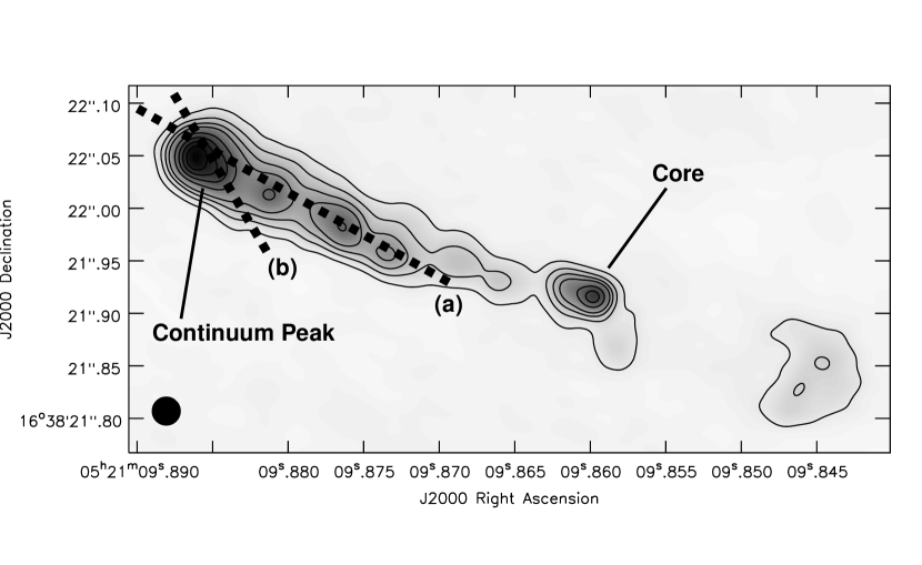
Figure 1: VLBA 21cm continuum image of 3C 138 with 20 mas resolution from Epoch III (2002). The black contours are at 10, 30, 60, 100, 200, 300, 400, 500, and 600 mJy beam^-1. The peak flux density is 607 mJy beam^-1 and the rms noise is 0.95 mJy beam^-1. The 60 mJy beam^-1 contour level is used for a continuum cutoff in subsequent optical depth discussions. The cross-cuts labeled (a) and (b) are described in §3.2.

The 21 cm continuum image of 3C 138 from the Epoch III (2002) data is shown in Figure 1. The resolution of this image is 20 mas and the rms noise is 0.95 mJy beam^-1. The brighter parts of the continuum morphology are in fair agreement with that presented in Faison et al. (1998), given that the current image has four times better S/N. The low surface brightness 21 cm (1.42 GHz) continuum morphology of Figure 1 is in excellent agreement with the 15 $\times$ 5 mas resolution, 1.7 GHz VLBI image presented by Cotton et al. (1997). Based on Cotton et al. (1997) the component just to the SW of image center is the core, while the linear structure to the northeast is the approaching part of the jet. The low surface brightness component in the SW corner of the image is the receding jet. These authors also review previous observations of 3C 138 and find that the source as a whole is not significantly variable. Cotton et al. (also see 2003) used high resolution multi-epoch VLBA data at 5GHz to demonstrate that the core components change by a few tens of mJy beam^-1 on timescales of $\sim 2$ years (note that the multiple core components detected by Cotton are unresolved at 20 mas resolution).

In order to test for variability in our 21 cm VLBA data, we constructed difference maps between the continuum images of each epoch. These maps show that indeed the “core” changes from epoch to epoch by $\sim 50$ mJy beam^-1, while the rest of the source is constant to within $\sim 10$ mJy beam^-1. Note that variability will not impact our optical depth calculations since: (1) the continuum appropriate for each epoch was used in the optical depth calculations; (2) no amplitude self-calibration was transfered from epoch to epoch; and (3) the intrinsic continuum morphology at 20 mas resolution does not change from epoch to epoch (according to Cotton et al., 2003, positional changes in the core components over eight years only amounts to $\lesssim 1.7$ mas, and these components are themselves not resolved by our 20 mas resolution data).

It is notable that our continuum peak flux densities for all three epochs of $\sim 605$ mJy beam^-1 (see Table 1) are about $30\%$ lower than that reported by Faison et al. (1998) (the images have the same resolution). The integrated flux of our data (including the re-reduction of the Epoch I data) is also low: $\sim 6.5$ Jy compared to 8.5 Jy reported in Faison et al. (1998). It is most likely that the previous data reduction is in error, given that the VLA 1.4 GHz flux density of 3C 138 is $\sim 8.5$ Jy (VLA calibrator manual), and it is very unlikely that a VLBA image could recover so much of the flux of such an extended source. Indeed, Cotton et al. (1997) also recover $\sim 70\%$ or (5.4 Jy) of the expected VLA flux in their 1.7 GHz VLBA image. We suspect that the use of a point source model in FRING during the earlier data reduction (Faison et al., 1998) coupled with details of the self-calibration are to blame for these discrepancies. We are confident that the current method of data reduction is valid, and in any case this difference will not affect the optical depths presented below since the continuum was extracted from the line free parts of the H I data, and all three of our epochs (including re-reduction of 1995 data) agree within a few percent.

3.2 H I Optical Depths

Figure 2 shows the average Epoch III (2002) optical depth profile along with the difference between the average Epoch III and Epoch II spectra. It is clear from this figure that the H I spectrum is rich and complex toward 3C 138 despite its high latitude ($b=11.3\arcdeg$). Overall, the average spectra are quite similar with significant deviations only occurring in the narrow velocity component near 6 km s^-1 and in a broader component near $-7$ km s^-1.

Heiles & Troland (2003a) recently completed the “Millennium Arecibo 21 cm Absorption Line Survey” toward 79 continuum sources, including 3C 138. As part of their study these authors have made detailed Gaussian fits to the Arecibo H I data, being careful to separate Galactic emission from absorption. Since 3C 138 is significantly smaller than the Arecibo beam at 21cm ($\sim 3\arcmin$), the effective resolution is equal to the size of 3C 138. Thus comparison of our 20 mas resolution data to the Arecibo spectrum provides an interesting check on whether or not the physical conditions of the gas change on scales of order $\sim 800$ mas (see for example MERLIN image in Davis et al., 1996). For example, a change in the spin temperature should be apparent in the line widths.

To first order, the Heiles & Troland Arecibo absorption spectrum is quite similar to our VLBA spectra. Therefore, we have used their results as the initial guesses for our own Gaussian analysis. The center velocities were initially held fixed at the Heiles & Troland (2003a) values, and then varied slightly to improve the residuals. The maximum residual in our optical depth fit occurs near $V_{LSR}\sim+7$ km s^-1 and has a value of 0.04. Table 2 shows the results of our analysis for the H I spectra at the continuum peak of the Epoch III data along with the Arecibo results for comparison (Heiles & Troland, 2003a). A Gaussian analysis for spectra of this complexity is unlikely to be unique, although, our results are in very good agreement with those obtained by Heiles & Troland for the four strongest components. However, although Heiles & Troland (2003a) were able to adequately fit their spectrum with 6 Gaussians, a seventh component at $\sim-7$ km s^-1 was needed to fit the VLBA spectrum. Interestingly, this is also one of the two regions where there is a significant deviation between the average Epoch III and Epoch II VLBA spectra (see Fig. 2). The Arecibo data were taken closest in time to the Epoch II data, and the $\sim-7$ km s^-1 was indeed less noticeable then. Although we have included it in our fit in order to directly compare with the Heiles & Troland results, the reality of the broad, weak component near $\sim+1.9$ km s^-1 is rather dubious.

Overall, the agreement between the VLBA data and Arecibo is quite impressive in center velocity, line width, and $\tau$. Although we only present Gaussian fitting results from the 2002 continuum peak, neither the center velocity or line width changes significantly as a function of position or epoch. That is, only the optical depth varies significantly from position to position and across epochs (these variations are described in more detail in §3.4).

Using the average H I spin temperature derived by Heiles & Troland (2003a) for the 3C 138 absorption components of $\sim 50$ K, we find that the average 2002 VLBA total H I column density is $\sim~{}6\times 10^{20}$ cm^-2. For this computation we have ignored the broad $+1.9$ km s^-1 component mentioned above (also see Table 2) since its reality seems doubtful. For comparison the H I column density observed in emission in the Arecibo data is $\sim~{}9.1\times 10^{20}$ cm^-2. Interestingly, given the normal assumption that $N_{TOT}\sim 2\times 10^{21}A_{v}$ and using $A_{v}\sim 1$ toward 3C 138 (NED database; Schlegel, Finkbeiner, & Davis, 1998) it is clear that much of the total hydrogen column toward 3C 138 is atomic since the combined warm plus cold H I column density can account for most of the total hydrogen column. Indeed, since 3C 138 is optically visible (Spinrad et al., 1985), $A_{v}\sim 1$ is likely an upper limit to the extinction strengthening this conclusion.

3.3 Zeeman Magnetic Field Limits

From the high S/N 1999 and 2002 H I data obtained in this study, we have also attempted to measure the Zeeman effect. That is, Stokes V = RCP-LCP; Stokes I= RCP+LCP and in the presence of a magnetic field $V=ZB_{\mathrm{los}}dI/2d\nu$, where Z=2.8 Hz $\mu$G^-1, and $B_{los}$ is the line of sight field strength. After careful inspection of the Stokes V cubes for both epochs, we do not find any convincing Zeeman signatures that meet both of the following criteria: (1) Stokes V larger than $5\sigma$ simultaneously in $both$ epochs; and (2) Stokes V more than $5\sigma$ over more than one beam width. The Stokes V spectral line rms noise levels are the same as those given in Table 1 for Stokes I.

Near the continuum peak for the component with highest S/N at $\sim 6$ km s^-1, we find $3\sigma$ upper limits for both epochs to $B_{los}$ of $\sim 45$ $\mu$G per pixel, with similar upper limits near the core (see Fig. 1). This upper limit is similar to the $2\sigma$ limit reported by Faison et al. (1998), but on a pixel by pixel basis rather than for an averaged profile. If instead we use profiles that have been averaged for pixels with absorption deeper than $-0.05$ mJy beam^-1, we find an average $3\sigma$ upper limit of 20 $\mu$G. Using the “Millennium Arecibo 21 cm Absorption Line Survey” data described in $\S 3.3$, Heiles & Troland (2004) find $B_{los}$$=+5.6\pm 1.0$ $\mu$G for the $\sim 6.4$ km s^-1 component, consistent with our averaged upper limit.

A number of recent VLA and VLBA Zeeman results suggest that the observed magnetic field strength often increases with higher resolution due to blending of spectral components at poorer resolution and beam dilution (i.e. higher fields averaged together with lower field regions or oppositely directed fields averaged within the beam; Brogan & Troland, 2001; Sarma, Troland, & Romney, 2001). The results presented here suggest that the Arecibo magnetic field results are not strongly affected by spectral blending (as already implied by the close agreement between the spectral profiles presented in §3.2) or beam dilution effects. Speculation on the significance of these low magnetic field detections and upper limits is provided in §4.3.3.

3.4 Small Scale Structure

For the remaining analysis of the small scale H I structure, we focus our attention on the 0.9, 6.2, and 9.1 km s^-1 velocity channels, since they are representative of the four strongest velocity features (see Fig. 2 and Table 2).

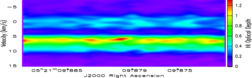
Figure 3: Position-Velocity diagram from the Epoch III (2002) data along the cross-cut labeled (a) in Figure 1.

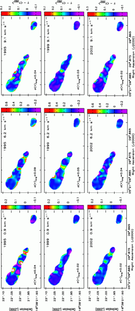
Figure 4: Optical depth channel maps minus the average value of the 2002 optical depth ($\tau-<\tau_{2002}>$) with velocity increasing to the right and time increasing down. The color scale for a given velocity is constant for each epoch. The color scale has been adjusted so that the dark blue color is centered about zero. The 2002 average optical depth values that were subtracted are: 0.34 at 0.9 km s^-1, 1.02 at 6.2 km s^-1, and 0.47 at 9.1 km s^-1 (Table 2). For reference the average value of the $1\sigma$ uncertainty in $\tau$ ($\sigma(\tau)_{avg}$) is indicated in the lower left hand corner. Note that while the 1995 data seem to have the largest variations, these data are also noisier by a fact of $\sim 2$ than the 1999 or 2002 data. Thus, it is very important to take into account the noise estimates when interpreting this Figure. For further discussion of the uncertainties see §3.4 and Table 2.

A position-velocity image for the Epoch III (2002) data along the cross-cut labeled (a) in Figure 1 is shown in Figure 3. It is clear from this image that there are discrete regions of higher and lower optical depth at constant velocities. Optical depth velocity channel maps are presented in Figure 4 for three different velocities: 0.9, 6.2, and 9.1 km s^-1 for all three epochs. The average value of the 2002 optical depth (for each channel) has been subtracted from the channel maps displayed in Figure 4. The difference in regions of higher and lower optical depth from epoch to epoch in these images is striking. To aid in assessing the significance of the optical depth variations presented in Figures 3 and 4, Table 3 lists the average $\tau$, along with the minimum, maximum, and mean values of the optical depth $error$ for each epoch for the 0.9, 6.2, and 9.1 km s^-1 channels. As with any optical depth map, the uncertainty in the optical depths shown in these figures is a non-linear function that is inversely proportional to the continuum brightness and proportional to the depth of the absorption. The minimum S/N ratio of the optical depths displayed in Figures 3 and 4 is 7 (which occurs near edges of the continuum), while near the continuum peak the S/N is more than 100.

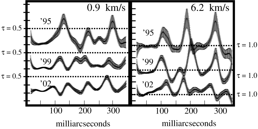
Figure 5: Optical depth cross-cuts at 0.9 and 6.2 km s^-1 along the position marked (a) in Figure 1 for all three epochs. The vertical tic mark interval is 0.1 and the width of the shaded line is equal to $\pm 1\sigma$, where $\sigma$ is the uncertainty in the measurement of $\tau$. This figure shows that the typical linear distance between significant H I variations is 50 mas.

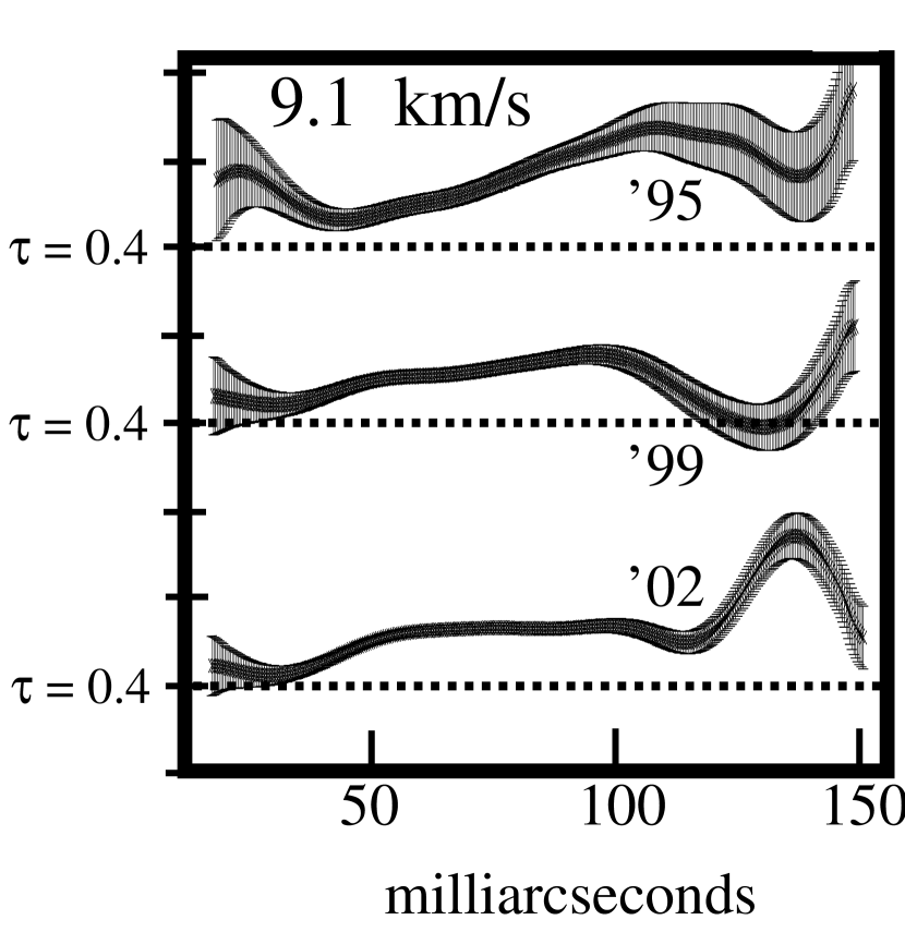
Figure 6: Optical depth cross-cuts at 9.1 km s^-1 along the position marked (b) in Figure 1 for all three epochs. The vertical tic mark interval is 0.05 and the width of the shaded line is equal to $\pm 1\sigma$, where $\sigma$ is the uncertainty in the measurement of $\tau$. This Figure is an example of of a cross-cut where no significant variations are observed.

Figure 5 shows an example of both spatial and temporal H I opacity variations across 3C 138 at 0.9 and 6.2 km s^-1, along the position angle indicated by the dashed line in Fig. 1 marked (a). The width of the shaded region indicates the $\pm 1\sigma$ uncertainty in the optical depth measurements. A number of H I optical depth “clumps” vary from the mean by more than $5\sigma$. The typical linear distance between significant variations is $\sim 50$ mas. The temporal variations between the three epochs are also striking along this cross cut. The variations along cross-cut (a) are particularly significant since it avoids the edges of the continuum where the optical depth uncertainties are greatest. For comparison, Figure 6 shows a cross cut along the position angle marked (b) in Figure 1. Clearly in this direction there are no significant spatial or temporal variations.

Since the weighting, $u-v$ coverage, and self-calibration for the line and continuum data for a given epoch are the same, the enhancements of the optical depths within a a given epoch (above the noise threshold) are almost certainly real. For example, if the line data were actually spatially smooth and the optical depth enhancements within a given epoch were dominated by subtle differences between the cleaning of the line and continuum images for the same epoch, the enhancements should look the same at each velocity within a given epoch and they do not (note that each channel of the line cubes was cleaned to the same flux level).

The possibility for “technical issues” (i.e. small changes in the $u-v$ coverage, flux, or imaging) to affect the appearance of the optical depth maps from epoch to epoch are greater (although the data reduction steps described in §2 should minimize these effects). However, if small changes in the continuum morphology from epoch to epoch were responsible for the temporal changes, the variations with time should mimic the continuum difference maps described in §2 and they do not. As a specific example, there is a 50 mJy beam^-1 difference between the continuum flux density at the peak of the ‘core’ component (see Fig. 1) due to intrinsic variability (Cotton et al., 2003) between the 1999 and 2002 data, yet the optical depth channel maps shown in Figure 4 for all three velocities at the location of the core are very similar between these two epochs (to within the stated $\sigma(\tau)$ noise levels). Also, apart from the core component, the 2002 continuum is consistently higher than the 1999 continuum (although the difference is not consistent with a simple zero point offset). However, for all three velocity components, the optical depths are not at all consistent with this trend (i.e. 1999 $\tau$ consistently higher than 2002; Figs. 4 and 5). Indeed, difference maps of the 2002 and 1999 optical depths look nothing like the continuum difference maps, and are instead very well correlated with the spectral line difference maps.

These comparisons demonstrate that the line to continuum ratios and hence optical depths are insensitive to changes in the continuum, as expected (i.e. the line changes commensurately, except where there is a real enhancement). Assessment of the effect of small changes in the $u-v$ coverage or imaging on the line data independent from those apparent in the continuum images from epoch to epoch is more difficult. However, there is no reason to believe that these effects would be greater than those described for the continuum data. Therefore, it is likely that the temporal variations are real.

4 DISCUSSION

4.1 Filling Factor of Small Scale H I

Current theoretical interpretations of the nature of the TSAS predict different values for the filling factor of such gas. Heiles (1997) predicts that, essentially independent of the geometry of the small-scale structures, their volume filling factor would be approximately 3%. Consequently, one would expect a comparable fraction of lines of sight to show opacity variations. On the basis of simulations of the H I power spectrum, Deshpande (2000) predicts that optical depth variations of order 0.2 over transverse scales of $\sim 100$ AU would be expected approximately 10% of the time.

Given the extended nature of 3C 138 and high signal to noise of the data presented in this work, it is possible to observationally constrain the covering fraction of the TSAS. We use the term ‘covering fraction’ to indicate that we cannot directly estimate the volume filling factor, only the fraction of 3C138 covered by TSAS along the line of sight. For the Epoch II and III data we have estimated the fraction of pixels exhibiting significant H I opacity variations for the 0.9 and 6.2 km s^-1 channels. We define a significant opacity change as $\Delta\tau=\mid\tau-\langle\tau\rangle\mid>5\sigma_{\tau}$. In this relation $\tau$ is the measured opacity at each pixel and $\langle\tau\rangle$ is the mean opacity over the source. The uncertainty in $\Delta\tau$ is estimated from adding in quadrature the average rms uncertainty of $\tau$ and the uncertainty in calculating the mean: $\langle\tau\rangle$. The total uncertainty is, of course, dominated by the average rms uncertainty in $\tau$. Table 3 lists these uncertainties for the 0.9 and 6.2 km s^-1 channels for Epochs II and III. Figure 7 shows histograms of the number of pixels as a function of $\Delta\tau$ for the 0.9 and 6.2 km s^-1 channels for Epochs II and III. For each histogram, the bin size is equal to $1\sigma_{\tau}$ (see Table 3).

With our conservative constraint of $\Delta\tau>5\sigma_{\tau}$ we find that the covering fraction of H I opacity significantly deviating from the mean for 1999 are: $5\%$ at 0.9 km s^-1 and $11\%$ at 6.2 km s^-1. For 2002 the covering fractions are: $7\%$ at 0.9 km s^-1 and $\sim 10\%$ at 6.2 km s^-1. From this analysis, we assume a typical covering fraction of $\sim 10\%$.

Although we cannot similarly measure the (volume) filling factor it must necessarily be significantly less than the covering fraction of $\sim 10\%$. The range of plane-of-sky physical sizes for the clumps of TSAS range from 5 to 25 AU (for distances between 100 to 500 pc (§2); and a typical angular size of 50 mas). Thus, even for aspect ratios of $\sim 10:1$ a single TSAS enhancement only spans $\sim 10^{-6}$ of the total line of sight. However, the TSAS is likely contained within the cold neutral medium (CNM) which itself only occupies a small fraction of the total line of sight. Recall that since 3C 138 is optically visible (§3.2), most of the CNM is comprised of H I along this line of sight, and thus the Aricebo H I column density likely traces the bulk of the CNM in this direction. If we assume that the average density of the large scale cold H I is 56 cm^-3 (i.e. as also assumed by; Heiles & Troland, 2003b, based on pressure arguments) and use the total cold H I column density toward 3C 138 of $6\times 10^{20}$ cm^-2 (§3.2), then all of the large size scale cold H I gas toward 3C 138 only occupies $\sim 3.5$ pc along the line of sight (compared to 500 pc extent of the Galactic H I disk in this direction). The line of sight depth of a single velocity component will be even less (assuming its density is equal to or higher than 56 cm^-3). Since TSAS is observed in all of the velocity components with sufficient signal to noise to detect it, it seems reasonable to divide the CNM path length by the number of velocity components (seven). From these numbers a lower limit to the filling factor of TSAS in the CNM along the line of sight to 3C 138 is $\sim 0.1\%$. Thus, while we emphasize that we cannot measure this value directly, a TSAS filling factor in the CNM of $\lesssim 1\%$ is plausible.

4.2 Pulsar Detection Simulations

As described in §1, contradictory results have been obtained from attempts to probe the Galactic TSAS with pulsars. These observations have prompted descriptions of small-scale H I structure ranging from potentially a relatively “rare phenomenon” (Stanimirović et al., 2003) to “a general property of the [interstellar medium]” (Frail et al., 1994). However, one difficulty with the pulsar observations is that although they have been sampled on timescales similar to that presented in this study toward 3C 138 (timescales of a couple of years), as well as significantly shorter timescales of a few months, they probe only discrete lines of sight. As a simple example, consider a pulsar moving behind a discrete H I clump. With “poorly chosen” epochs of observation, the pulsar lines of sight could bracket the clump and display little or no change in the optical depth.

Our observations cover a continuous range of angular scales from 20 to 300 mas, which includes the scales sampled typically by pulsar observations. Since the typical size scale of significant H I opacity variations toward 3C 138 is $\sim 50$ mas (see Figures 4 and 5) we use this value as the fiducial transverse sample scale. Using this typical separation we can assess the extent to which multi-epoch pulsar H I observations produce “typical” optical depth variations.

A single pulsar “trial” is simulated by forming the optical depth difference $\Delta\tau$ for two points separated by 50 mas along a cross-cut parallel to the long axis of 3C138 (see Figures 1 and 5). The angular extent of the long axis is sufficiently long that multiple “trials” can be simulated along the cross cut; the trials are made independent by moving the endpoints at least 20 mas (1 beam width) along the cross cut. Moreover, 3C138 is sufficiently wide along its short axis (SE/NW direction) that multiple, independent (i.e., offset by at least 20 mas from each other) cross cuts parallel to the long axis can be formed. Finally, we conducted pulsar simulation trials at all three velocities, 0.9, 6.2, and 9.0 km s^-1. In total, we were able to simulate 120 pulsar observation trials.

Figure 8 shows the resulting histogram of $\Delta\tau$ values for all independent pulsar simulations. It is apparent that the most probable value for $\Delta\tau$ is 0, but that there is a tail to large values, $\Delta\tau\gtrsim 0.3$. Based on these limited simulations, we expect that $\Delta\tau<0.1$ in $\sim 90\%$ of pulsar observations. Our simulated results are in reasonable agreement with the recent observational results by Stanimirović et al. (2003) and Johnston et al. (2003) who find that few pulsars show measurable $\Delta\tau$ changes. Moreover, the rapid temporal variations implied by our data toward 3C 138 will further reduce the probability of detecting variations with pulsar observations. Thus, drawing conclusions from pulsar observations about the fraction of the neutral ISM in small-scale H I structures is difficult due to the low probability that the observing epochs will be exactly matched to the size scale (and timing) of an appreciable variation in $\Delta\tau$.

4.3 Significance of Spatial and Time Variations

4.3.1 Is the Line of Sight to 3C 138 Special?

Two of the most notable aspects of the H I absorption toward 3C 138 (catalog 3C) is the relatively large amplitude of opacity variations observed and that observed variations have a fairly uniform typical sizescale of 50 mas ($\sim 25$ AU). While opacity variations are observed toward other sources (Faison et al., 1998; Faison & Goss, 2001) in many cases, these opacity variations are much smaller in amplitude. To what extent is the line of sight to 3C 138 (catalog 3C) typical of other lines of sight through the ISM?

Table 4 summarizes the H I absorption observations in the literature that have made use of VLBI imaging. There is a clear bimodal distribution for the sizes of sources that have been studied, with only 3C 138 (catalog 3C) and 3C 147 (catalog 3C) probing length scales larger than 100 AU. In contrast, from Figure 5, it is clear that for the case of 3C 138 (catalog 3C)  the typical size scale for significant changes is $\sim 50$ mas. There are of course uncertainties in converting between the observed angular scales and the equivalent linear scales, as in many cases the Galactic H I rotation curve is of limited utility in determining the distance to the absorbing gas. Nonetheless, it is clear that only two sources, 3C 138 (catalog 3C) and 3C 147 (catalog 3C), are both large enough and have a high enough surface brightness to make the detection of these opacity variations significant.

We conclude that the the large amplitude opacity variations that are observed toward 3C 138 (catalog 3C) and 3C 147 (catalog 3C) are likely to be a selection effect. Much like the case of the pulsar observations (§4.2), the typical equivalent linear scales probed by the lines of sight to most sources are too small to have a large probability of displaying a significant opacity variation.

4.3.2 What is the Nature of the Small Scale H I Gas?

There are two main explanations for the small scale H I gas: (1) the variations are caused by changes in the physical properties of small parcels of gas; or (2) the variations are merely the manifestation of random fluctuations contributed by the entire range of spatial scales in the ”red” H I power spectrum.

In the past, the main argument against a “physical entity” interpretation for the small scale structure has been the difficulty in reconciling the pressure that such “clumps” would exert on the surrounding medium. Heiles (1997) has attempted to ameliorate the pressure problem by suggesting that the temperature of the small scale features is low compared to the average ISM, and that they have a filamentary or sheet like structure, so that the density is also lower than implied by the transverse size. However, we have shown in §3.2 that there is little difference between the line widths of the VLBA spectra and that obtained by Heiles & Troland (2003a) using the Arecibo telescope toward 3C 138. Indeed, the VLBA line widths are slightly wider than their Arecibo counterparts (see Table 3).

This comparison seems to exclude the possibility that the small scale features have significantly lower temperatures. For example, Heiles & Troland (2003a) estimate from comparison of the Arecibo absorption and emission spectra that the H I spin temperatures of the four strongest 3C 138 velocity components range from 40 to 55 K. These spin temperatures translate into thermal line widths of 1.3 to 1.6 km s^-1 (using $\Delta V_{th}=0.214T^{0.5}$). The difference between the observed line width and the thermal width is presumably due to turbulent motions in the gas. If the spin temperature dropped to $\sim 15$ K in the small scale structures as suggested by Heiles (1997), we would expect to see a decrease in the VLBA line widths of $\sim 0.5$ to 0.8 km s^-1 compared to the Arecibo spectrum. Such changes are well within the sensitivity of the Gaussian fitting for the strong components, and are not observed. It is possible that a drop in spin temperature is exactly countered by a large increase in the turbulent width, but this seems unlikely. Thus, the absence of line-width decreases in the VLBA data indicates that the dominant cause of the opacity variations is likely to be density fluctuations, possibly accompanied by a small increase ($\lesssim 0.3$ km s^-1) in the thermal or turbulent contributions to the line widths. Such an increase in the thermal or turbulent widths would account for the somewhat greater widths of the stronger VLBA lines compared to the Arecibo data (Table 2).

Jenkins & Tripp (2001) have carried out a comprehensive survey of the UV lines of C I in the directions of 21 early type stars near longitudes of $100\arcdeg$ and $300\arcdeg$ with distances in the range of 1 to 3.7 kpc. The C I lines arise from the three fine-structure levels of the ground electronic state. Based on ratios of the two excited levels, it is possible to derive the pressures in the interstellar medium. A small fraction of the sight lines probed by Jenkins & Tripp (2001) show evidence for significantly enhanced pressures. Jenkins (2004) has summarized these results and suggests that rapid changes in pressure may arise from the cascade of mechanical energy to small scales from larger scales. The pressure changes occur over time scales much shorter than the time required for thermal equilibrium to be established. Jenkins & Tripp (2001) suggest that one of the motivations for Heiles (1997) to attribute the H I small scale structure to lower temperature sheets or filaments viewed edge-on can be eliminated. That is, the objection to small scale structures based on excessive H₂ formation and thus excessive extinction can be avoided with time scale considerations; H₂ molecular formation does not have time to occur. Thus the overpressure problem, which was the main impetus for Heiles’ suggestions, is solved precisely because these structures are not in equilibrium and their lifetime is short. The volume filling factor of the over pressured ISM, as determined from the C I lines, is a few percent at most ($\sim 3.7\%$ Jenkins & Tripp, 2001; Jenkins, 2004), comparable to the low filling factors of enhanced H I optical depth implied by the low covering fraction of such gas toward 3C 138 (see §4.1). To summarize, only a small fraction of the total H I mass is located in these fluctuations, which is consistent with various other analysis such as that by Dickey & Lockman (1990). These density fluctuations are almost certainly far from equilibrium and short-lived.

Currently, only Deshpande (2000) has attempted the difficult task of extending the H I power spectrum down to size scales relevant to the VLBA opacity variations described here. Unfortunately, there are a number of unresolved issues regarding the Deshpande (2000) extrapolation that call into question its direct applicability to the current observational data. Foremost among these issues is that the observed H I power spectrum used in the Deshpande (2000) study (toward CasA) only covers one decade in spatial scale, while the extrapolation is over four decades of spatial scales. As also pointed out by Deshpande (2000), the extrapolation is very sensitive to the assumed spectral index. Indeed, the CasA model with a slope of $-2.75\pm 0.25$ (Deshpande et al., 2000) predicts peak optical depth variations that are $\sim 5$ times less than we observe (0.5) toward 3C 138. Moreover, Deshpande et al. (2000) observed significantly different power law indices for the line of sight toward Cas A and one of the two clouds toward Cygnus A, suggesting that the power spectrum may depend on direction (see also Green, 1993; Dickey et al., 2001).

These observed differences are potentially crucial given that according to Deshpande (2000), a change of just 0.1 in the power law spectral index would imply a change in the expected opacity variations on AU scales by a factor of $\sim 2$. Also, if the neutral ISM is dominated by filamentary or sheet-like structures (as one might expect if the density fluctuations are transient features arising from shocks), the effective spectrum of the density fluctuations could be significantly different than assumed. Further detailed investigation into these issues on small scales will have to await analysis of the observed H I power spectrum toward 3C 138 down to scales of at least 10 AU. It is entirely possible that using the appropriate power spectrum for 3C 138, the Deshpande (2000) model could produce results that are in agreement with the level of opacity fluctuations described in this paper.

It is notable that the power law slope determined by (Deshpande et al., 2000) and assumed by Deshpande (2000): $-2.75$ is quite shallow compared to that expected from pure Kolmogorov turbulence of $\sim-3.7$. Recent theoretical work by Lazarian & Pogosyan (2000, 2004) suggests that if the velocity, as well as the density structure of the gas are properly taken into account, the Kolmogorov slope is modified to shallower values (between $-2.67$ to $-3.4$) depending on whether velocity or density fluctuations dominate the power spectrum. The shallowest values correspond to the velocity dominated case. Indeed, Lazarian & Pogosyan (2000, 2004) suggest that as the velocity averaging of H I data is increased, the effect of velocity will be reduced and the slope should steepen. For H I observed in emission, Dickey et al. (2001) (in the Galaxy) and Stanimirović & Lazarian (2001) (in the SMC) do find evidence of this effect, i.e. the power spectrum slope steepens as the velocity averaging of the data is increased. However, (Deshpande et al., 2000) do not see evidence of this effect in their H I absorption data. Dickey et al. (2001) also find that the degree of steepening as a function of velocity averaging is much less for the cooler H I components in their emission line data compared to the hotter gas. These observational results are in general agreement with Lazarian & Pogosyan (2004) who find that opacity effects can play a role in the resulting power spectrum slope, beyond the effects of velocity or density dominance. Thus, overall it seems likely that all current H I power spectrum analysis from both emission and absorption data (including Deshpande, 2000) are consistent with a modified Kolmogorov like turbulence.

The fundamental difference between the Jenkins and Deshpande pictures is that the latter ascribes the small scale fluctuations to “red” noise (noise that increases at larger spatial scales) in the H I power spectrum with contributions from all spatial scales (i.e. optical depth changes are statistical and not due to physical changes in the gas), while the former suggests that a cascade of mechanical energy creates short lived small physical regions with high pressures. Our detections of 2-d optical depth enhancements or “clumps” (see Figs. 4, 5 for example) makes the Deshpande picture seem less likely. Note that this argument would be stronger, even definitive if the clumps with typical sizes of $\sim 50$ mas were more significantly larger than the beam size of 20 mas. Future, higher resolution observations and simulations may help to resolve this issue. Currently, a paradigm based on a Kolmogorov like turbulent or mechanical cascade which produces regions of enhanced pressure does seem favorable based on the recent theoretical and optical work, in addition to our new H I optical depth data, although it is quite possible that both phenomena contribute to the observed opacity differences.

4.3.3 Significance of Zeeman Non-detections

The Arecibo Millennium survey provides the highest sensitivity statistical look at the magnetic field strength in a large sample of cold neutral medium (CNM) clouds to date (Heiles & Troland, 2004, 2005; Heiles & Crutcher, 2005), including the direction of 3C 138. For H I components with either significant $B_{los}$ detections (22) or significant upper limits ($\sigma<10$ $\mu$G; 47), these authors find that (1) the median total magnetic field strength is $6\pm 1.8$ $\mu$G; (2) the median non-thermal contribution to the linewidth is $\sim 2.8$ km s^-1 (velocity dispersion $\sim 1.2$ km s^-1); (3) there are no strong correlations of $B_{los}$ with H I column density, linewidth, or spin temperature (but the dispersion of these parameters is also fairly small); and (4) the magnetic and turbulent energies are in approximate equilibrium (also see similar results in Myers et al., 1995). Indeed, using the parameters from (1), (2), and $B=0.4\Delta V_{NT}n^{0.5}$ (obtained by setting the magnetic and turbulent energies equal, see for example Crutcher et al., 2003; Myers & Goodman, 1988) we find that the density is $\sim 30$ cm^-3 in agreement with that expected from pressure equilibrium arguments (Heiles & Troland, 2003b). In the above equation $\Delta V_{NT}$ is the non-thermal contribution to the FWHM linewidth in km s^-1 and $n$ is the proton density in cm^-3. Specifically for the 3C 138 6.2 km s^-1 component, Heiles & Troland (2004) derive $B_{los}$$=+5.6\pm 1.0$ $\mu$G, and $\Delta V_{NT}=2.1$ km s^-1 (assuming that the thermal contribution has $T_{s}\sim 40$ K); this value is also consistent with equipartition between the magnetic and turbulent energies on large sizescales for this line of sight if $n\sim 50$ cm^-3.

To avoid potential confusion we note that a similar correlation between the magnetic field strength and density also exists for dense molecular clouds with $B\propto\Delta Vn^{0.5}$ (Basu, 2000; Crutcher et al., 2003). However, for self-gravitating clouds it is unclear whether this relation is the result of equipartition between the magnetic and turbulent energies (which has also been observed for this density regime) or depends on the details of gravity, geometry, and ambipolar diffusion. The observed relation can be derived equally well from both possible lines of argument; Heiles & Crutcher (2005) provide a review of this outstanding question and we will not address it further here.

As described in §3.2 and §4.3.2 the small scale H I optical depth enhancements cannot be due to changes in the non-thermal linewidths. If small scale H I structures are interpreted as density enhancements, densities of $\sim 10^{5}$ cm^-3 are required (see §1). Using the non-thermal linewidth of the 6.2 km s^-1 component of $\Delta V=2.1$ km s^-1, magnetic and turbulent equipartition implies that the magnetic field strength should be on the order of 250 $\mu$G for $n\sim 10^{5}$ cm^-3 – well within our $3\sigma$ single pixel detection limit (45 $\mu$G; §3.2). This analysis suggests that magnetic and turbulent equipartition does not exist on very small sizescales. However, since flux freezing almost certainly exists in the cold neutral medium (see for example Heiles & Crutcher, 2005) it is difficult to imagine a scenario whereby a large change in the density of the small scale H I structures – on the order of two to three orders of magnitude – would not result in an appreciable change in the magnetic field strength. We speculate that the lack of observed increase in field strength expected from equipartition may be due to an inability of MHD waves to propagate at these sizescales; MHD waves with frequencies higher than the ion-neutral collision frequency cannot propagate (see for example Nakano, 1998). For a CNM cloud size of $\sim 3.5$ pc (§4.1), ionization fraction $10^{-4}$ (Heiles & Crutcher, 2005), and Alfvén velocity of $\sim 2.1$ km s^-1 (i.e. using the non-thermal linewidth), the cutoff wavelength is on the order of 10 AU similar to the sizescale of the VLBA H I features. Simulations are needed to explore in detail whether this or other possible scenarios are plausible.

4.3.4 Do the H I Structures Move or Reform?

Obviously it is impossible with only three epochs of data separated in time by a few years to answer this question. From Figure 5, it is clear that the small scale H I structures certainly do change on timescales of $\lesssim 3-4$ years. It is tempting to assign at least some of the temporal variations visible in Fig. 5 to physical movement of the H I “clumps” (optical depth enhancements). For example, if the first clump of the 1995 6.2 km s^-1 data shown in Fig. 5 at a relative position of $\sim 70$ mas along the cross-cut is the same feature apparent in the 1999 data at $\sim 150$ mas, and the 2002 data at $\sim 240$ mas, the “clump” is moving with a transverse velocity of $\sim 20$ km s^-1. Other similar apparent motions of H I “clumps” across the three epochs can also be imagined. If real, such motions, which are highly supersonic, could be indicative of shocks. Whether the observed enhancements are then due to the clumps themselves moving or if enhancements reform in new parcels of gas as the shock front itself moves (i.e. akin to the debate regarding maser spots) is a matter for further speculation and debate, and is beyond the scope of this work. We note that the small increases seen in the VLBA line widths toward 3C 138 compared to Arecibo data (discussed in §4.3.2) provide weak support for a shock model. It is also possible to reconcile the temporal variations observed toward 3C 138 with the Deshpande (2000) picture (where small scale variations are due to contributions from all spatial scales) if the large scale H I clouds are moving with appreciable transverse velocities (A. Deshpande, private communication).

5 SUMMARY AND CONCLUSIONS

We have presented new H I absorption observations of 3C 138 (catalog 3C) from 2002 with the VLBA and the re-analysis of two earlier epochs in 1995 and 1998. We find significant spatial and temporal variations in the H I optical depth ($\Delta\tau>0.1$) across the face of 3C 138 (catalog 3C). The spatial variations are similar to the levels found by Faison & Goss (2001), but our signal-to-noise ratio is much improved.

The spatial variations of the H I optical depth occur on a typical angular scale of 50 mas and have maximum values of $\sim 0.5$. Assuming that the absorbing gas is at a distance of no more than 500 pc, the equivalent linear size is $\lesssim 25$ AU. The total (CNM) H I column density toward 3C 138 (assuming a spin temperature of 50 K) is $6\times 10^{20}$ cm^-2. Significant time variations are seen from epoch to epoch, indicating a typical time scale of no more than a few years. We have also searched for the Zeeman effect in the 1999 and 2002 data. We place a ($3\sigma$) upper limit of approximately 45 $\mu$G at the 3C 138 continuum peak and a ($3\sigma$) upper limit of 20 $\mu$G for the averaged H I profile. We find an average plane of sky covering factor for the small scale H I gas of $\sim 10\%$ toward 3C 138; the total volume filling factor must necessarily be much smaller. A plausible number for the filling factor of TSAS in the CNM (which itself only occupies $\sim 1\%$ of the total line of sight) is $1\%$. We do not find any evidence for a narrowing of the VLBA H I line widths compared to single dish measurements. This suggest that small scale variations in the H I opacities are not caused by changes in the spin temperature.

Because of their high velocities, multi-epoch observations of pulsars would appear to be a way to sample different lines of sight and search for H I opacity variations. Employing this technique, a variety of pulsar observations have found conflicting results. We have simulated a set of pulsar observations by forming the differences of the H I opacity across the face of 3C 138 (catalog 3C) on an angular scale comparable to that probed by the pulsar observations. While we can find significant opacity variations on a small number of differenced lines of sight, these occur only with a low probability. Quantitatively, our simulation is in good agreement with the fraction of pulsar observations reporting significant opacity variations. We conclude that pulsar observations, unless they are sampled much more often and over longer durations than has been the case heretofore, may be of limited utility in characterizing small-scale opacity variations.

We currently favor the Jenkins (2004) interpretation for the nature of the small scale H I gas, although the Deshpande (2000) interpretation may also be viable if a power spectrum appropriate for the 3C 138 direction is determined in the future. In the Jenkins picture, the small scale structure arises from pressure driven density enhancements due to the cascade of mechanical energy from large to small scales. The recent theoretical work of Lazarian & Pogosyan (2000) suggests that the observed power law slopes observed by Deshpande et al. (2000) and others is in agreement with a revised picture of Kolmogorov turbulent cascade. The short lifetime of these structures removes the need to explain away the TSAS with low temperatures or as merely “fluctuations” in the H I power spectrum. We hesitate to dismiss the notion that the structures are filamentary or sheet-like, since evidence for such structures is quite ubiquitous at larger size scales in recent observations of the ISM from optical (WHAM) to radio wavelengths (SGPS).

There are a number of future lines of research that would help shed light on the intriguing results for TSAS presented in this paper. In particular, a sensitive VLBA H I monitoring program of the 3C 138 line of sight on short timescales of perhaps a month would help to determine the timescale for variation. Similar observations toward other large bright quasars (3C 147 for example) would help to determine the ubiquity of the H I variations observed toward 3C 138. Based on our experiences, we recommend that these observations be carried out with phase referencing to remove the ambiguities introduced by self-fringing on the target source. A time variability monitoring program for the optical fine structure lines would also be interesting. A power spectrum from large (100pc) to small (10 AU) sizescales should be constructed for the H I gas toward 3C 138 using existing VLA, MERLIN, and VLBA data, and compared in detail with the predictions of the Deshpande model. Theoretical constraints/predictions for the timescale and level of density contrast possible from a Kolmogorov-like cascade would also provide useful comparisons with the observational data. It seems likely that such a cascade would require a high frequency cutoff (corresponding to small spatial scales) in order to produce a strong density contrast and hence the TSAS – such a cutoff may also explain the typical sizescale of TSAS observed in the data presented here of $\sim 50$ mas ($\sim 25$ AU). For example, some form of MHD waves may provide such a small scale cutoff, since these waves cannot propogate at frequencies higher than the ion-neutral collision rate.

Figure 2: Average optical depth profile from the Epoch III (2002) data (dotted). The three velocity components discussed in the text are labeled for reference. The solid line shows the difference between the average 2002 and average 1999 optical depth profiles (i.e. $\tau_{\rm Avg{2002}}-\tau_{\rm Avg1999}$)

.

Figure 7: Plot of the number of pixels in the (a) Epoch II 0.9 km s^-1, (b) Epoch III 0.9 km s^-1, (c) Epoch II 6.2 km s^-1, and (d) Epoch III 6.2 km s^-1 opacity images as a function of $\Delta\tau=\mid\tau-\langle\tau\rangle\mid$. The bin size is equal to the $1\sigma$ uncertainty in $\Delta\tau$ (see Table 3). The total number of pixels sampled is 5693 and 5837 for the Epoch II and Epoch III data, respectively. The percentage of pixels with $\Delta\tau\gtrsim 5\sigma$ is $5\%,7\%,11\%$, and $10\%$ for panels (a)-(d) respectively.

Figure 8: Simulation of the $\Delta\tau$ variations that would be observed by 120 pulsar observations with epochs separated by the equivalent of 50 mas (typical size scale of H I opacity variations, see Fig. 4). The beginning and end points of the observations are randomly selected from the cross-cut labeled (a) in Figure 1 as well as two parallel positions separated by a beam width.

Table 1: Observational Parameters

Parameter	Epoch I	Epoch II	Epoch III
Date	10 Sept 1995	22 Dec 1999	12 May 2002
Number of IFs	4	4	4
Bandwidth per IF (MHz)	0.25	0.5	0.5
Spectral channels	128	256	256
Channel separation (km s-1)	0.41	0.41	0.41
Velocity resolutiona (km s-1)	0.82	0.82	0.82
Clean Beamd (mas)	18.7 x 13.6 ($-$0.7)	17.9 x 10.3 ($-$6.5)	19.7 x 14.5 (3.5)
Continuum Peak (mJy beam-1)	610	600	607
Continuum rms noise (mJy beam-1)	1.1	0.88	0.95
Spectral line rms noise (mJy beam-1)	3.0	1.8	1.6
General Parameters for 3C 138
Positionb (J2000)	$05^{\rm h}21^{\rm m}09\fs 904$,	$+16\arcdeg 38\arcmin 22\farcs 116$
Positionc (Galactic)	$+187.4\arcdeg$,	$-11.34\arcdeg$
Redshift	0.759

Table 2: Results From H I Gaussian Analysis

	2002 VLBAa				2000 Arecibob,c
$V_{LSR}$ (km s-1)	$\Delta V$ (km s-1)	$\tau^{d}$		$V_{LSR}$ (km s-1)	$\Delta V$ (km s-1)	$\tau^{e}$
$-$21.5	$2.8\pm 0.8$	0.02		$-$21.5	$3.5\pm 0.2$	0.04
$-$7.3	$2.1\pm 0.9$	0.02		-	-	-
$-$0.4	$3.3\pm 0.1$	0.27		$-$0.5	$2.9\pm 0.1$	0.25
+1.7	$2.1\pm 0.1$	0.13		+1.6	$1.8\pm 0.1$	0.18
+1.9	$19.0\pm 1.0$	0.07		+1.8	$14.6\pm 0.5$	0.06
+6.4	$2.56\pm 0.02$	0.93		+6.4	$2.30\pm 0.02$	1.05
+9.1	$2.87\pm 0.05$	0.37		+9.1	$2.81\pm 0.06$	0.46

Table 3: Uncertainties in H I Optical Depths

Epoch	Velocity (km s-1)	$\langle\tau\rangle$	Min. $\tau$ errora	Max. $\tau$ errora	Avg. $\tau$ error ($\sigma_{\tau}$)
1995	0.9	0.34	0.007	0.09	0.04
	6.2	1.11	0.014	0.40	0.09
	9.1	0.50	0.009	0.11	0.04
1999	0.9	0.34	0.004	0.05	0.02
	6.2	1.07	0.009	0.28	0.05
	9.1	0.47	0.005	0.06	0.03
2002	0.9	0.34	0.003	0.04	0.02
	6.2	1.02	0.007	0.13	0.04
	9.1	0.47	0.004	0.05	0.02

Table 4: VLBI H I Absorption Measurements toward Compact Extragalactic Sources

	Galactic	H I Gas	Flux	Angular	Linear	Largesta	Largest
Name	latitude	Distance	Density	Resolution	Resolution	Angular Scale	Linear Scale	Ref.
	(°)	(pc)	(Jy)	(mas)	(AU)	(mas)	(AU)
3C 119 (catalog 3C)	$-4$	$<500$	8.6	10	5	50	25	2
3C 138 (catalog 3C)	$-11$	$<500$	8.5	20	10	400	200	1
3C 147 (catalog 3C)	$+10$	500–1000	22.5	10	10	190	200	2
B0404$+$768 (catalog )	$+18$	$<320$	5.8	10	3	100	30	1
B0831$+$557 (catalog )	$+36$	200	8.8	20	4	160	30	2
B2255$+$416 (catalog )	$-16$	$<360$	2.1	10	4	40	16	1
B2352$+$495 (catalog )	$-12$	$\approx 1300$	2.4	10	13	50	70	2

References. — (1) Faison et al. (1998); (2) Faison & Goss (2001)

References

- Arzoumanian et al. (2002) Arzoumanian, Z., Chernoff, D. F., & Cordes, J. M. 2002, ApJ, 568, 289
- Basu (2000) Basu, S. 2000, ApJ, 540, L103
- Brogan & Troland (2001) Brogan, C. L. & Troland, T. H. 2001, ApJ, 560, 821
- Clifton et al. (1988) Clifton, T. R., Frail, D. A., Kulkarni, S. R., & Weisberg, J. M. 1988, ApJ, 333, 332
- Cotton et al. (2003) Cotton, W. D., Dallacasa, D., Fanti, C., Fanti, R., Foley, A. R., Schilizzi, R. T., & Spencer, R. E. 2003, A&A, 406, 43
- Cotton et al. (1997) Cotton, W. D., Dallacasa, D., Fanti, C., Fanti, R., Foley, A. R., Schilizzi, R. T., & Spencer, R. E. 1997, A&A, 325, 493
- Crutcher (1999) Crutcher, R. M. 1999, ApJ, 520, 706
- Crutcher et al. (2003) Crutcher, R., Heiles, C., & Troland, T. 2003, Lecture Notes in Physics, Berlin Springer Verlag, 614, 155
- Davis et al. (1996) Davis, R.J., Diamond, P.J., & Goss, W.M. 1996, MNRAS, 283, 1105
- Deshpande (2000) Deshpande, A.A. 2000, MNRAS, 317, 199
- Deshpande et al. (2000) Deshpande, A.A., Dwarakanath, K.S., & Goss, W.M. 2000, ApJ, 543, 227
- Deshpande et al. (1992) Deshpande, A. A., McCulloch, P. M., Radhakrishnan, V., & Anantharamaiah, K. R. 1992, MNRAS, 258, 19P
- Diamond et al. (1989) Diamond, P.J., Goss, W.M., Romney, J.D., Booth, R.S., Kalberla, P.M.W., & Mebold, U. 1989, ApJ, 347, 302
- Dickey et al. (2001) Dickey, J. M., McClure-Griffiths, N. M., Stanimirović, S., Gaensler, B. M., & Green, A. J. 2001, ApJ, 561, 264
- Dieter et al. (1976) Dieter, N.H., Welch, W.J., & Romney, J.D. 1976, ApJ, 206, L113
- Faison (2002) Faison, M.D. November 2002, Eds. A.R. Taylor, T.L. Landecker, & A.G. Willis. ASP Conference Proceedings Series, Vol. CS-276.
- Faison & Goss (2001) Faison, M.D. & Goss, W.M. 2001, AJ, 121, 2706
- Faison et al. (1998) Faison, M.D., Goss, W.M., Diamond, P.J., & Taylor, G.B. 1998, AJ, 116, 2916
- Frail et al. (1994) Frail, D. A., Weisberg, J. M., Cordes, J. M., & Mathers, C. 1994, ApJ, 436, 144
- Frail et al. (1991) Frail, D. A., Cordes, J. M., Hankins, T. H., & Weisberg, J. M. 1991, ApJ, 382, 168
- Green (1993) Green, D. A. 1993, MNRAS, 262, 327
- Heiles (1997) Heiles, C. 1997, ApJ, 481, 193
- Heiles & Crutcher (2005) Heiles, C. & Crutcher, R. M. 2005, in Magnetic Fields in the Universe, ed. R. Wielebinski, Springer, in press, astro-ph/0501550
- Heiles & Troland (2003a) Heiles, C. & Troland, T. H. 2003a, ApJS, 145, 329
- Heiles & Troland (2003b) Heiles, C. & Troland, T. H. 2003b, ApJ, 586, 1067
- Heiles & Troland (2004) Heiles, C. & Troland, T. H. 2004, ApJS, 151, 271
- Heiles & Troland (2005) Heiles, C. & Troland, T. H. 2005 astro-ph/0501550
- Jenkins (2004) Jenkins, E. B. 2004, Ap&SS, 289, 215
- Jenkins & Tripp (2001) Jenkins, E. B. & Tripp, T. M. 2001, ApJS, 137, 297
- Johnston et al. (2003) Johnston, S., Koribalski, B., Wilson, W., & Walker, M. 2003, MNRAS, 341, 941
- Lauroesch et al. (2000) Lauroesch, J.T., Meyer, D.M., & Blades, J.C. 2000, ApJ, 543, L43.
- Lauroesch et al. (1998) Lauroesch, J.T., Meyer, D.M., Watson, J.K., & Blades, J.C. 1998, ApJ, 507, L89.
- Lazarian & Pogosyan (2004) Lazarian, A., & Pogosyan, D. 2004, ApJ, 616, 943
- Lazarian & Pogosyan (2000) Lazarian, A. & Pogosyan, D. 2000, ApJ, 537, 720
- Lorimer et al. (1997) Lorimer, D. R., Bailes, M., & Harrison, P. A. 1997, MNRAS, 289, 592
- Marscher et al. (1993) Marscher, A.P., Moore, E.M., & Bania, T.M. 1993, ApJ, 419, L101
- Meyer & Lauroesch (1999) Meyer, D.M., & Lauroesch, J.T. 1999, ApJ, 520, L103.
- Moore & Marscher (1995) Moore, E.M., & Marscher, A.P. 1995, ApJ, 452, 671.
- Myers & Goodman (1988) Myers, P. C., & Goodman, A. A. 1988, ApJ, 329, 392
- Myers et al. (1995) Myers, P. C., Goodman, A. A., Gusten, R., & Heiles, C. 1995, ApJ, 442, 177
- Nakano (1998) Nakano, T. 1998, ApJ, 494, 587
- Rollinde et al. (2003) Rollinde, E., Boissé, P.,
- Sarma, Troland, & Romney (2001) Sarma, A. P., Troland, T. H., & Romney, J. D. 2001, ApJ, 554, L217 Federman, S.R., & Pan, K. 2003, å, 401, 215
- Schlegel, Finkbeiner, & Davis (1998) Schlegel, D. J., Finkbeiner, D. P., & Davis, M. 1998, ApJ, 500, 525
- Spinrad et al. (1985) Spinrad, H., Marr, J., Aguilar, L., & Djorgovski, S. 1985, PASP, 97, 932
- Stanimirović & Lazarian (2001) Stanimirović, S., & Lazarian, A. 2001, ApJ, 551, L53
- Stanimirović et al. (2003) Stanimirović, S., Weisberg, J. M., Hedden, A., Devine, K. E., & Green, J. T. 2003, ApJ, 598, L23
- Zauderer et al. (2002) Zauderer, B.A., Faison, M.D., Goss, W.M., Brogan, C., & DePree, C.G. November 2002, Eds. A.R. Taylor, T.L. Landecker, and A.G. Willis. ASP Conference Proceedings Series, Vol. CS-276.
.