XMM-Newton spectroscopy
of the metal depleted T Tauri star TWA~5

We present results of X-ray spectroscopy for TWA~5, a member of the young TW Hydrae association, observed with XMM-Newton. TWA~5 is a multiple system which shows H$\alpha$ emission, a signature typical of classical T Tauri stars, but no infrared excess. From the analysis of the RGS and EPIC spectra, we have derived the emission measure distribution vs. temperature of the X-ray emitting plasma, its abundances, and the electron density. The characteristic temperature and density of the plasma suggest a corona similar to that of weak-line T Tauri stars and active late-type main sequence stars. TWA~5 also shows a low iron abundance ($\sim 0.1$ times the solar photospheric one) and a pattern of increasing abundances for elements with increasing first ionization potential reminiscent of the inverse FIP effect observed in highly active stars. The especially high ratio ${\rm Ne/Fe}\sim 10$ is similar to that of the classical T Tauri star TW~Hya, where the accreting material has been held responsible for the X-ray emission. We discuss the possible role of an accretion process in this scenario. Since all T Tauri stars in the TW Hydrae association studied so far have very high ${\rm Ne/Fe}$ ratios, we also propose that environmental conditions may cause this effect.

1 Introduction

T Tauri stars are young late-type stars with an age of a few Myr, contracting toward the zero age main sequence phase (Feigelson & Montmerle 1999, and references therein). They are classified in two groups: classical T Tauri stars (CTTSs) and weak-line T Tauri stars (WTTSs). This classification is based on ${\rm H}\alpha$ emission. CTTSs show strong H$\alpha$ emission (${\rm EW}>10$ Å). They are still accreting material from their circumstellar disk, and broad and asymmetric ${\rm H}\alpha$ emission is a direct evidence of this process. In WTTSs H$\alpha$ emission is less strong, indicating that the accretion process has ended and the star is approaching the main-sequence. In most cases CTTSs are also characterized by an infrared excess which marks the presence of a circumstellar disk. The infrared excess is usually considered a prerequisite for accretion, but it does not imply that accretion actually takes place; in fact, some WTTSs also show an infrared excess although much fainter than in CTTSs. Since coeval CTTSs and WTTSs are often observed in the same star forming region, the duration of the accretion phase appears to be different from star to star.

Table 1: Characteristics of the sample of T Tauri stars, sorted by H$\alpha$ emission, for which high resolution X-ray spectra have been analyzed. In case of resolved multiple systems the stellar mass, spectral type, and bolometric luminosity refer to the component responsible for the X-ray emission.

Name	Mass	Spectral	EW(H$\alpha$)a	$L_{\rm X}^{\rm b}$	$\log(L_{\rm X}^{\rm b}/L_{\rm bol})$	$N_{\rm e}^{\rm c}$	Referencesd
	($M_{\odot}$)	Type	(Å)	${\rm(erg\,s^{-1})}$		${\rm(cm^{-3})}$
TW Hya	$\sim 0.7$	K7	-220.0	$1.3\times 10^{30}$	-2.7	$\sim 10^{13}$	1, 2, 3, 4
TWA 5	$\sim 0.5$	M1.5	-13.4	$6.7\times 10^{29}$	-3.1	$<10^{11}$	2, 5, 6
HD 98800	$\sim 1.1$	K5	0.0	$4.1\times 10^{29}$	-3.8	$\lesssim 10^{11}$	2, 7, 8
PZ Tel	$\sim 1.1$	K0	0.1	$2.2\times 10^{30}$	-3.2	$<10^{12}$	9, 10, 11
HD 283572	$\sim 1.8$	G5	1.1	$7.8\times 10^{30}$	-3.1	$\cdot\cdot\cdot$	12, 13, 14

^a Negative values of H$\alpha$ equivalent width mark an emission line. ^b X-ray luminosity evaluated in the $6-20$ Å band, using the XMM/MOS or Chandra/HETGS best fit models presented in the relevant papers. ^c Densities estimated from the O vii and Ne ix triplets. ^d Data from: (1) Batalha et al. (2002); (2) Reid (2003); (3) Stelzer & Schmitt (2004); (4) Kastner et al. (2002); (5) this work; (6) Jensen et al. (1998); (7) Kastner et al. (2004); (8) Prato et al. (2001); (9) Cutispoto et al. (2002); (10) Thatcher & Robinson (1993); (11) Argiroffi et al. (2004); (12) Strassmeier & Rice (1998); (13) Fernandez & Miranda (1998); (14) Scelsi et al. (2005).

One of the signatures of stellar youth is a high X-ray emission level. Many star forming regions have been under investigation in order to infer the properties of X-ray emission from pre-main-sequence (PMS) stars. One of the debated questions is whether and how the X-ray emission of accreting CTTSs and non accreting WTTSs differs. It is conceivable that the occurrence of the accretion process in CTTSs might play a role in determining the different X-ray emission characteristics. In fact, the circumstellar disk is thought to affect the geometry of the stellar magnetosphere (Königl 1991; Bouvier et al. 2003). Moreover accreting material may provide an alternative heating mechanism for the emitting plasma, although shock heated plasma cannot attain temperatures higher than a few MK. The picture emerging from the analysis of low resolution X-ray spectra of PMS stars is that the X-ray luminosity of CTTSs is lower than that of WTTSs, and the X-ray spectra produced by CTTSs appear harder than WTTS spectra (Neuhäuser et al. 1995; Stelzer & Neuhäuser 2000; Tsujimoto et al. 2002; Flaccomio et al. 2003; Stassun et al. 2004; Ozawa et al. 2005). The harder X-ray spectra of CTTSs may be explained with the presence of plasma hotter ($T\sim 10-100$ MK) than that of WTTSs ($T\sim 10$ MK, Tsujimoto et al. 2002). If this is the case, the shock heating mechanism cannot be responsible for the X-ray emission in CTTSs. However, it is also possible that circumstellar material absorbs the softest part of the X-ray radiation, simulating therefore a higher temperature in CTTSs (Stassun et al. 2004).

Table 2: Log of the XMM observation of TWA~5 (Rev. 565, ObsId 0112880101).

Instrument	Science	Filter	Start	Exposure	Count Rate
	Mode		(UT)	(ks)	(${\rm cts\,s^{-1}}$)
PN	Full Frame	Medium	2003 Jan 9 03:28:56	27.9	1.68
MOS1	Full Frame	Medium	2003 Jan 9 03:06:55	29.5	0.45
MOS2	Full Frame	Medium	2003 Jan 9 03:06:55	29.5	0.46
RGS1	Spectroscopy	…	2003 Jan 9 03:06:03	29.7	0.06
RGS2	Spectroscopy	…	2003 Jan 9 03:06:03	29.7	0.08

High resolution X-ray spectra, such as those obtained today with grating spectrometers on board XMM-Newton and Chandra, offer the possibility to reconstruct the emission measure distribution ($EMD$) of the emitting plasma, to measure its abundances, and to constrain the electron density $N_{\rm e}$. These diagnostics help to improve our understanding of the X-ray emission from accreting and non accreting young stars. However, to achieve a good $S/N$ ratio in these spectra, bright and nearby sources are needed. The TW Hydrae association (TWA, Zuckerman et al. 2001, and references therein) is one of the nearest ($\sim 55\,{\rm pc}$) and youngest ($\sim 10\,{\rm Myr}$) star forming regions and therefore its members are ideal targets for the analysis of X-ray emission from PMS stars by means of high resolution spectroscopy. In the present paper we report on the XMM-Newton observation of TWA~5 (CD $-33\degr 7795$). High resolution X-ray spectra of PMS stars have been analyzed in sufficient detail so far for only four other stars: TW~Hydrae (TW Hya or TWA 1), HD~98800 (TWA 4), PZ~Tel and HD~283572. TW~Hydrae and HD~98800, together with TWA~5, are members of the TWA; PZ~Tel and HD~283572 belong to the $\beta$-Pictoris moving group and to the Taurus-Auriga star forming region, respectively.

This paper is organized as follows: in Sect. 2 the principal characteristics of TWA~5 and of the other PMS stars used for comparison are reported; Sect. 3 presents the main information about the XMM-Newton observation of TWA~5 and the methods adopted for the data analysis; in Sect. 4 we report the results derived, which are discussed and compared with properties of other PMS stars in Sect. 5; we draw our conclusions in Sect. 6.

2 Star Sample

TWA~5 is a quadruple system located $\sim 55$ pc from the Sun. The primary, TWA~5A, is a triple system: a $0\aas@@fstack{\prime\prime}06$ binary resolved by adaptive optics (Macintosh et al. 2001; Brandeker et al. 2003), one of the visual components being itself a spectroscopic binary (Torres et al. 2001). All three of them have similar spectral types (M1.5). The secondary, TWA~5B, is a brown dwarf separated by $2\arcsec$ from the primary (Lowrance et al. 1999; Webb et al. 1999). TWA~5A does not show any infrared excess indicating no significant amount of circumstellar material (Metchev et al. 2004; Weinberger et al. 2004; Uchida et al. 2004). On the other hand, Mohanty et al. (2003) measured H$\alpha$ emission typical of accreting PMS stars and signatures of outflows, and concluded that at least one of the components in the TWA~5A system is a CTTS. It remains currently unclear how the accretion signatures can be reconciled with the lack of evidence of a disk. Moreover it is unknown whether the X-ray emitting component of TWA~5A coincides with the accreting one.

Table 1 summarizes the relevant stellar parameters for TWA~5 and the other stars, that we will use for comparison in our study.

TW~Hya is a single CTTS with enhanced ${\rm H}\alpha$ emission (equivalent width $\sim 200$ Å, Alencar & Batalha 2002; Reid 2003) and strong infrared excess (Uchida et al. 2004). Its X-ray emission, observed with Chandra/HETGS (Kastner et al. 2002) and XMM-Newton (Stelzer & Schmitt 2004), shows peculiar features: the emitting plasma has quite a low temperature ($\log T{\rm(K)}\sim 6.5$), the ${\rm Ne/Fe}$ abundance ratio is as high as a factor 10 in solar photospheric units, and the electron density $N_{\rm e}$, derived from the He-like triplets of O vii and Ne ix, is $\sim 10^{13}\,{\rm cm^{-3}}$, more than two orders of magnitude above that of typical stellar coronae. Based on these peculiarities it was suggested that X-ray emission from TW~Hya is produced in an accretion shock rather than in a corona. On the other hand, Drake (2005) has pointed out that the He-like emission line triplets may be affected by photoexcitation due to the UV radiation field. If this were the case the triplet $f/i$ ratio would overestimate the density in the emitting region.

HD~98800 is a WTTS quadruple system, composed by two visual components HD~98800A and HD~98800B (whose separation is $0\aas@@fstack{\prime\prime}8$), each of which is a spectroscopic binary. It has been observed with Chandra/HETGS (Kastner et al. 2004); from this observation it emerged that its X-ray emission is due mainly to HD~98800A, and it is produced by plasma at temperatures in the range $\log T{\rm(K)}\sim 6.4-7.0$, with ${\rm Ne/Fe}\sim 5$, and low electron density ($N_{\rm e}<10^{12}\,{\rm cm^{-3}}$), typical of stellar coronae.

PZ~Tel and HD~283572 are two single WTTSs. The X-ray spectrum of PZ~Tel, gathered with Chandra/HETGS, has been analyzed by Argiroffi et al. (2004). The X-ray spectrum of HD~283572, observed with both Chandra/HETGS and XMM-Newton, has been studied by Audard et al. (2005) and by Scelsi et al. (2005). For both PZ~Tel and HD~283572 a typical coronal plasma emerged, with temperatures of $\sim 10$ MK, and with ${\rm Ne/Fe}\sim 2-3$ times the solar photospheric ratio.

3 Observation and Data Analysis

TWA~5 was observed for $\sim 30$ ks with XMM-Newton on 2003 January 9. In Table 2 we report the observation log for all the instruments.

Both EPIC and RGS data have been processed with SAS V5.4.1 standard tools. We have extracted EPIC source events from a circle with radius of $60^{\prime\prime}$, centered on the target position. This extraction circle includes 90% of the source encircled energy. Background events have been extracted from an annular region around the target with inner and outer radii of $60^{\prime\prime}$ and $90^{\prime\prime}$. The observation is not affected by significant background contamination due to solar flares and therefore no time screening was required. We have also verified that EPIC spectra are not affected by significant pile-up. The spectral analysis has been performed by adopting the Astrophysical Plasma Emission Database (APED V1.3, Smith et al. 2001), which assumes ionization equilibrium according to Mazzotta et al. (1998).

Figure 1: XMM-Newton/PN light curve of TWA~5 with bin size of 500 s.

3.1 EPIC Data Analysis

The PN light curve of TWA~5 (Fig. 1) does not show strong flare-like events, but an unbinned Kolmogorov-Smirnov test applied to the PN photon arrival times yields a probability of $2\times 10^{-7}$ related to the hypothesis of constant emission. This result indicates the presence of significant small amplitude variability. The observed PN and MOS spectra are shown in Fig. 2. We have fitted separately the PN and MOS spectra in the energy range $0.3-7.9$ keV, assuming an absorbed optically-thin plasma model with three thermal components. We have also left as free parameters the abundance of those elements (O, Ne, Mg, Si, S, Fe, and Ni) which significantly improved the fit, while the abundances of the remaining elements (C, N, Al, Ar, and Ca) were tied to the Fe abundance. We have performed the fitting by using XSPEC V11.3.0. The uncertainty on each best-fit parameter, at the 68% confidence level, has been computed by exploring the $\chi^{2}$ variation while varying simultaneously all the other free parameters. From the PN best-fit model we have derived an estimate for the hydrogen column density, $N_{\rm H}\sim 3\times 10^{20}\,{\rm cm^{-2}}$, and the same value has been found as an upper limit from the analysis of the MOS spectra. This result indicates that the spectra of TWA~5 do not suffer strong absorption. The derived $N_{\rm H}$ value is compatible with that assumed by Jensen et al. (1998), which agrees with the negligible extinction toward the TWA region. The results obtained from the PN and MOS spectral fitting are reported in Table 3.

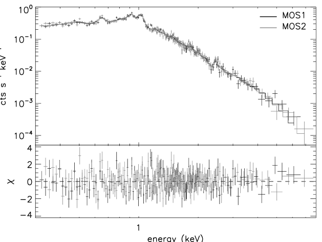
Figure 2: EPIC spectra (PN in upper panel, MOS1 and MOS2 in lower panel) of TWA~5 with best-fit 3-$T$ models superimposed. The lower section of each panel contains residuals. Best-fit parameters are reported in Table 3.

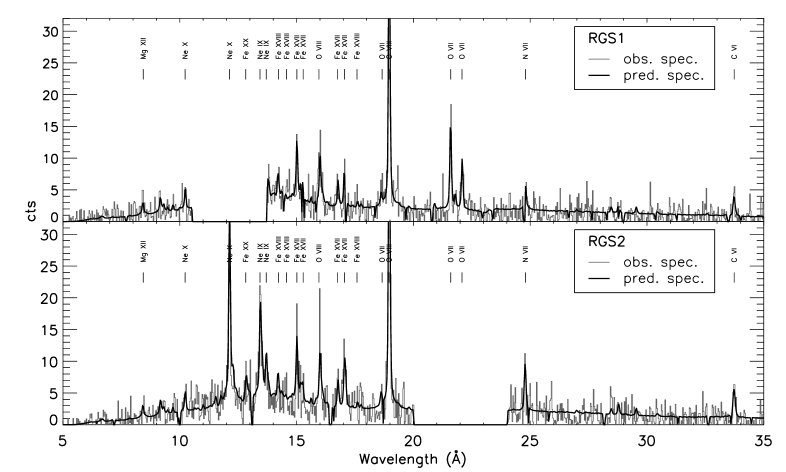
Figure 3: Observed and predicted RGS spectra (rebinned with a wavelength bin of 0.03 Å) of TWA~5.

Table 3: TWA~5 best fit paramenters.

	PN	MOS	RGS
	Abundancesa,b ($A_{X}/A_{X\sun}$)
C	$={\rm Fe}$	$={\rm Fe}$	$0.26^{+0.30}_{-0.08}$
N	$={\rm Fe}$	$={\rm Fe}$	$0.55^{+0.61}_{-0.18}$
O	$0.15^{+0.11}_{-0.07}$	$0.28^{+0.14}_{-0.14}$	$0.31^{+0.29}_{-0.07}$
Ne	$0.34^{+0.27}_{-0.16}$	$0.93^{+0.37}_{-0.51}$	$0.92^{+0.74}_{-0.26}$
Mg	$0.07^{+0.15}_{-0.06}$	$0.14^{+0.20}_{-0.13}$	$0.51^{+0.16}_{-0.38}$
Si	$0.21^{+0.20}_{-0.16}$	$0.19^{+0.22}_{-0.15}$	$={\rm Fe}$
S	$0.32^{+0.36}_{-0.31}$	$0.36^{+0.38}_{-0.32}$	$={\rm Fe}$
Fe	$0.05^{+0.04}_{-0.02}$	$0.09^{+0.06}_{-0.05}$	0.1
Ni	$1.08^{+1.17}_{-0.98}$	$0.06^{+1.31}_{-0.06}$	$={\rm Fe}$
	Temperatureb (K)
$\log T_{1}$	$6.17^{+0.56}_{-0.20}$	$6.56^{+0.14}_{-0.14}$
$\log T_{2}$	$6.70^{+0.17}_{-0.05}$	$6.90^{+0.19}_{-0.25}$
$\log T_{3}$	$7.27^{+0.09}_{-0.06}$	$7.27^{+0.33}_{-0.09}$
	Emission Measureb $N_{\rm e}N_{\rm H}V\;({\rm cm^{-3}})$
$\log EM_{1}$	$52.71^{+0.79}_{-0.63}$	$52.45^{+0.60}_{-0.37}$
$\log EM_{2}$	$53.21^{+0.26}_{-0.31}$	$52.76^{+0.34}_{-0.70}$
$\log EM_{3}$	$52.72^{+0.10}_{-0.26}$	$52.64^{+0.15}_{-0.30}$
	Column Densityb (${\rm 10^{20}cm^{-2}}$)
$N_{\rm H}$	$2.8^{+3.9}_{-2.5}$	$\leq 3.3$	$=1$
	Best Fit Statistics
$\chi^{2}_{\rm red}$	0.89	0.99
d.o.f.	404	285
$P(\chi^{2}>\chi^{2}_{\rm obs})$	94%	54%

• Solar photospheric abundances are from Anders & Grevesse (1989).

• All the uncertainties correspond to the 68% confidence level.

3.2 RGS Data Analysis

The RGS1 and RGS2 spectra of TWA~5 are shown in Fig. 3. The analysis has been performed using ISIS (Houck & Denicola 2000) and PINTofALE (Kashyap & Drake 2000). Our approach is to derive $EMD$ and abundances starting from the line flux measurements. It is known that the line spread function of the RGS spectra is characterized by large wings, making it difficult to identify correctly the continuum level and therefore to measure line fluxes. In order to obtain accurate line flux measurements we have evaluated the continuum level by performing a global fit of the RGS1 and RGS2 spectra. We have adopted a model composed of three isothermal components with variable abundances of C, N, O, Ne, Mg and Fe. The continuum predicted on the basis of this best-fit model has been used to measure the fluxes of the strongest RGS emission lines. To improve the spectral $S/N$ ratio we have measured the line fluxes by fitting simultaneously RGS1 and RGS2 spectra rebinned with a 0.03 Å wavelength bin. These line fluxes are reported in Table XMM-Newton spectroscopy of the metal depleted T Tauri star TWA~5.

We have reconstructed the $EMD$ and element abundances with the Markov-Chain Monte Carlo (MCMC) method of Kashyap & Drake (1998) applied to the measured line fluxes. This method performs a search in the $EMD$ and abundances parameter space with the aim of maximizing the probability of obtaining the best match between observed and predicted line fluxes. Some of the main advantages of this method are that it does not need to assume a particular analytical function for the $EMD$, and that it allows to estimate uncertainties on each $EMD$ and abundance value. On the basis of the formation temperature of the selected set of lines, we have adopted a temperature grid ranging from $\log T{\rm(K)}=6.0$ to $\log T{\rm(K)}=7.3$, with resolution $\Delta\log T{\rm(K)}=0.1$, over which to perform the $EMD$ reconstruction. We have assumed a hydrogen column density $N_{\rm H}=10^{20}\,{\rm cm^{-2}}$, compatible with the values derived from the analysis of the EPIC spectra (see Sect. 3.1). In Fig. 4 we show the comparison between the observed line fluxes and those predicted on the basis of the $EMD$ and abundances derived with the MCMC method.

Figure 4: Comparison between observed and predicted line fluxes in the RGS spectra. The predicted values are obtained using the models derived with the MCMC method (see Sect. 3.2).

Table 4: Total counts (lines + continuum) in the interval 10-30 Å band vs. Fe abundance.

	$N_{\rm pred}$					$N_{\rm obs}$
${\rm Fe/Fe_{\sun}}^{\rm a}$	0.05	0.07	0.10	0.15	0.20
RGS1	2298	1841	1498	1232	1099	1377
RGS2	2886	2379	1998	1702	1554	1874

• Abundance referred to the solar photospheric value from Anders & Grevesse (1989).

Since line fluxes depend on the product of the $EMD$ with the element abundances, the adopted method provides the $EMD$ scaled by the Fe abundance, and the abundance ratio of each element with respect to Fe. However, it is worth noting that the continuum emission, depends strongly on the amount of emission measure, and weakly on the absolute abundances of elements heavier than He. In fact the continuum emission is due to three processes: bremsstrahlung radiation, radiative recombination and two-photons emission. For the temperatures involved in the plasma of TWA~5 the main contribution to the continuum is due to bremsstrahlung radiation which depends very weakly on the heavy element abundances. Therefore, after performing the MCMC reconstruction, we have considered several models assuming different absolute Fe abundances and therefore different global scaling factors for the $EMD$ distribution. For each of these models we have compared the predicted and observed continuum levels. Since it is hard to identify correctly the continuum level in RGS spectra, as already mentioned above, we have also compared the observed and predicted total emission (spectral lines + continuum) as a further check. In Table 4 we report the explored Fe abundances, and the corresponding total counts for the simulated spectra $N_{\rm pred}$, to be compared with the observed total number of counts, $N_{\rm obs}$. With this procedure we have determined the absolute Fe abundance, and therefore the absolute position of the $EMD$ and the absolute abundances of all the other elements. The resulting Fe abundance is $0.1$ times the solar photospheric value of Anders & Grevesse (1989), with an uncertainty smaller than a factor 2. As a final cross-check, we have verified that the predicted continuum level agrees with the continuum used for the line flux measurements. The abundances resulting from the RGS analysis are reported in Table 3.

4 Results

The X-ray luminosity of TWA~5, computed in the interval $6-20$ Å from the best-fit models of PN, MOS and RGS spectra, is 8.3, 6.7 and $6.7\times 10^{29}\,{\rm erg\,s^{-1}}$, respectively. The derived luminosities are compatible within the best-fit parameter errors. As shown by Tsuboi et al. (2003), from a Chandra/ACIS-S observation, the X-ray emission is essentially due to the primary TWA~5A. In fact the Chandra observation was able to resolve the brown dwarf TWA~5B from the primary TWA~5A, and Tsuboi et al. measured for TWA~5B an X-ray luminosity of $4\times 10^{27}\,{\rm erg\,s^{-1}}$.

Figure 5: Emission measure distribution of TWA~5 obtained from the RGS line fluxes with the MCMC method, along with the values obtained with the 3-$T$ best-fit model of PN and MOS spectra. The uncertainties correspond to 68% statistical confidence level.

4.1 Emission Measure Distribution

In Fig. 5 we report the $EMD$ vs. temperature derived from the EPIC and RGS spectral analysis of TWA~5. All the instruments detect the strongest thermal component at $\log T{\rm(K)}\sim 6.7-7.0$, but the RGS spectra are not able to probe the hottest plasma component at $\log T{\rm(K)}\sim 7.3$, detected by EPIC. The reason of this result is the different effective area of EPIC and RGS in the hardest part of the X-ray spectra ($E\ga 2$ keV). In principle, the high-temperature tail could be probed by exploiting a number of Fe xxii-xxiv lines, which fall in the wavelength region $10.7-11.8$ Å  covered by RGS, but the emissivity of these lines is relatively low and the RGS resolution too poor for this purpose.

4.2 Abundances

In Fig. 6 (and in Table 3) we show the element abundances, in solar photospheric units (Anders & Grevesse 1989), derived from the spectra obtained with each instrument. The elements are sorted along the abscissa by increasing values of first ionization potential (FIP). The abundances of C and N, which have their strongest emission lines in the low-energy part of the observed spectral range ($\lambda\sim 25-35$ Å, or $E\sim 0.35-0.5$ keV), are derived only from the RGS. On the other hand, the abundances of Si and S are estimated only from the EPIC spectra since their H-like and He-like lines fall at high energies, and they cannot be constrained by the RGS. Note that the Fe abundance derived from RGS data has been estimated with a procedure (Sect. 3.2) which does not allow to obtain a formal statistical uncertainty, however we are confident that it cannot be off by more than a factor 2, as explained in Sect. 3.2. We note that the abundances derived from different instruments are compatible within statistical uncertainties. However some systematic differences come out, as briefly discussed in Sect. 4.4. From the derived abundances it emerges that the X-ray emitting plasma of TWA~5 is metal depleted.

Figure 6: Abundances of TWA~5, with respect to solar photospheric values (Anders & Grevesse 1989), obtained using the RGS line fluxes with the MCMC method, along with the values obtained with the 3-$T$ best-fit model of PN and MOS spectra. The uncertainties correspond to the 68% confidence level, except the error bar of Fe derived from RGS data, which has been obtained with a different procedure, as discussed in Sects. 3.2 and 4.2.

4.3 Electron Density

We have evaluated the plasma electron density from the analysis of the O vii He-like triplet. The other He-like triplets which fall in the RGS spectral range were either too weak (N vi, Mg xi, Si xiii), or heavily blended with other strong lines (Ne ix) to be analyzed. In Fig. 7 we show the RGS1 spectrum (rebinned with a 0.03 Å bin size) in the O vii triplet region with superimposed the best-fit curves. The measured ratio of forbidden $f$ and intercombination $i$ line fluxes is $3.8\pm 2.5$ (see Table XMM-Newton spectroscopy of the metal depleted T Tauri star TWA~5 for line fluxes), which yields an upper limit of $\sim 10^{11}\,{\rm cm^{-3}}$ for $N_{\rm e}$, adopting the predicted $f/i$ ratios of Smith et al. (2001).

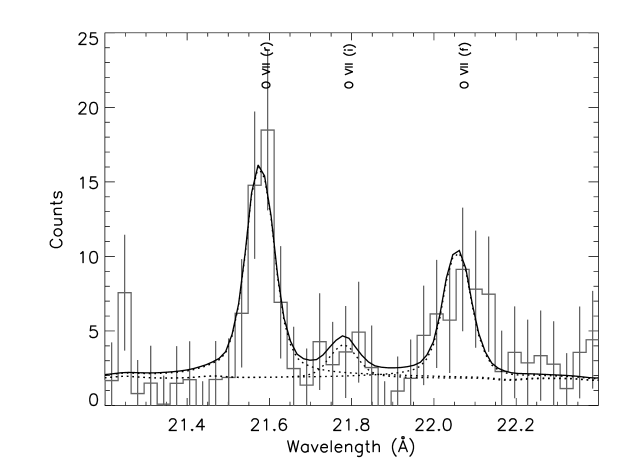
Figure 7: O vii triplet in the RGS1 spectrum of TWA~5, rebinned with a wavelength bin of 0.03 Å, with best-fit line profiles: individual lines (dotted line) and their sum (solid line).

4.4 Comparison between Different Models

We have performed separate analyses of the PN, MOS and RGS spectra for several reasons. The main reason is that an approach based on fluxes of selected individual lines, measurable only in the RGS data, provide us with the most reliable results for the element abundances and for the plasma $EMD$. Moreover, independent analyses of EPIC data offer the opportunity to compare the results of the different XMM-Newton instruments. These comparisons allow us to investigate the robustness of each measurement, and therefore they are useful to test the reliability of results based on EPIC data only, in the broader contest of observations of X-ray coronal sources with no high resolution spectrum available.

As already mentioned in Sect. 4.2, abundance estimation from different XMM-Newton instruments turns out to be quite robust, at least within the statistical uncertainties of a typical XMM-Newton observation ($\sim 30$ ks exposure time, in the present case). However, the abundances of Mg, Fe, O, and Ne obtained from the PN fitting are systematically lower than the corresponding values based on the analysis of the MOS and RGS spectra, which agree among themselves. On the other hand, the emission measure values derived from the PN analysis are larger than those obtained from the MOS and RGS spectra, and the X-ray luminosity predicted by the PN model is $\sim 20$% higher than in the other two cases. Although, all the differences are within the statistical uncertainties, it is conceivable that the higher spectral resolution of the MOS detector, with respect to the EPIC/PN, allows to disentangle better the contributions of lines and continuum, and therefore to constrain the absolute values of $EMD$ and abundances. Moreover, EPIC/MOS and RGS share the same X-ray telescopes and hence their cross-calibration is better determined, while residual calibration problems of the PN instrument may cause the differences in the fitting results described above.

EPIC models are able to provide a good global description of the source plasma, but limited to models with few free parameters, while RGS spectra allow to derive a more detailed model but – with the available signal to noise ratio – they fail to detect plasma components with temperatures higher than $T\geq 10$ MK, due to the smaller energy range covered by RGS with respect to EPIC.

In order to cross-check the three models we have compared each of them with the spectra of different XMM-Newton instruments and we have computed reduced $\chi^{2}$ values. The best-fit 3-$T$ models of PN and MOS globally describe RGS spectra reasonably well ($\chi^{2}_{\rm red}=1.8$ and $\chi^{2}_{\rm red}=1.3$ respectively, with 817 d.o.f.), but not as well as the line-based $EMD$ model ($\chi^{2}_{\rm red}=1.0$ with 817 d.o.f.). As already noticed the RGS model misses the higher temperature components and hence it underestimates the PN and MOS spectra at high energy. Finally, both RGS and MOS models show some disagreement with the PN spectrum in the low energy range.

5 Discussion

In this section we discuss the results obtained for TWA~5, in terms of $EMD$, abundances and density, and compare them with those for the CTTS TW~Hya, and the other WTTSs in our sample (Sect. 2). We stress that all results are based on high resolution X-ray spectra. It must be recalled that TWA~5A is a triple system, and so far we have not been able to determine whether the X-ray emission and the accretion signatures emerge from the same star.

The analysis of both the EPIC and RGS data has shown that the X-ray emission of TWA~5 is mainly produced by hot plasma ($T\sim 10$ MK). The analysis of the O vii triplet has indicated a typical coronal electron density ($N_{\rm e}\leq 10^{11}\,{\rm cm^{-3}}$). These characteristics are similar to those found in WTTSs (Kastner et al. 2004; Argiroffi et al. 2004; Scelsi et al. 2005) and magnetically active late-type main sequence stars when high resolution X-ray spectroscopy is used (see e.g. Ness et al. 2004). Peculiar features of TWA~5 are its very low metallicity (${\rm Fe/Fe_{\sun}}\sim 0.1$) and its extremely high abundance ratio ${\rm Ne/Fe}\sim 10$. Such high values for the ${\rm Ne/Fe}$ have been observed only in a few very active stars (HR~1099, UX~Ari, II~Peg) having average coronal temperatures larger than those of TWA~5 (see below), and it has been ascribed to the so-called inverse FIP effect (see discussion below). On the other hand, a low metallicity (${\rm Fe/Fe_{\sun}}\sim 0.2$) and the same Ne/Fe ratio have been measured for TW~Hya, the only unambiguous CTTS studied so far at high spectral resolution in X-rays. Hence, it is an interesting issue why TWA~5 shares the same chemical peculiarities with TW~Hya, in spite of having other thermal characteristics.

Figure 8: Ne/Fe abundance ratio in solar photospheric units (Anders & Grevesse 1989) for the PMS stars listed in Table 1 and sorted by H$\alpha$ equivalent width. We have assumed that the abundance uncertainties of HD~98800 are equal to those of TW~Hya, because the observed Chandra spectra of these two stars have similar $S/N$.

We recall that TW~Hya presents spectral characteristics compatible with a model of X-ray emission driven, or at least affected, by the infalling accretion stream (Kastner et al. 2002; Stelzer & Schmitt 2004). In fact, all the X-ray properties of TW~Hya (e.g. its low plasma temperature, high density, and metal depletion) suggest that the emitting plasma forms in the shock region where the infall streams reach the stellar surface. Among the peculiar characteristics of TW~Hya the very low abundances of all the metals in the emitting plasma appear to be compatible with the accretion scenario. In fact, Stelzer & Schmitt proposed that Fe and other heavy elements in the accretion disk condense into dust grains (see e.g. Savage & Sembach 1996) which possibly settle into the disk midplane, while other elements like N, remain in the gas phase. Neon and other noble elements, should also not remain locked onto dust grains, but rather be part of the gas phase (Frisch & Slavin 2003). Since the accreting material is largely composed by gas rather than dust (Takeuchi & Lin 2002), the accreting stream is expected to display a high Ne/Fe abundance ratio. This material falls onto the stellar surface and there, heated to temperatures of few MK by the ensuing shock, produces X-ray radiation revealing its anomalous chemical composition. The intriguing point is that TWA~5 presents exactly the same abundance ratios of TW~Hya, and in particular a ${\rm Ne/Fe}\sim 10$, but lacks all the other indications for accretion-related X-ray emission. In Fig. 8 we show the Ne/Fe ratio for the PMS stars in our sample. The stars are sorted along the abscissa by increasing value of H$\alpha$ equivalent width, in order to separate the accreting CTTSs, on the left part of the diagram, from the non accreting WTTSs. This plot suggests that CTTSs tend to have Ne/Fe higher than WTTSs.

As already hinted above the Ne/Fe ratio could be influenced also by FIP-related effects: in the solar corona, and in particular in long-lived active regions, and in late type stars with low activity levels, abundances of elements with low FIP appear to be enhanced with respect to the high FIP elements (see Feldman & Widing 2003, and references therein), using photospheric abundances as a reference. On the other hand, more active stars present an overabundance of high FIP elements with respect to low FIP elements, the so called inverse FIP effect (Brinkman et al. 2001; Drake et al. 2001; Audard et al. 2003). Early models to explain the FIP effect involve ion-neutral fractionation in the chromosphere (Geiss 1982; Meyer 1996), but they do not provide a satisfactory explanation for the selective enhancement of some elements in the corona (see Güdel 2004, for a recent review). Most recently, Laming (2004) has proposed a new model which tries to explain both a FIP and an inverse FIP effect as a result of the pondermotive forces related to chromospheric Alfvén waves acting on ions of different species. The Ne/Fe ratio is a good indicator of the coronal abundance pattern since Ne has a high FIP value (21.6 eV), while Fe is a low FIP element (7.9 eV), and strong lines from both elements have close wavelengths at similar coronal temperatures. Stars with high activity level usually show ${\rm Ne/Fe}\sim 1-5$, and only few active binaries present ${\rm Ne/Fe}\sim 10$ (Brinkman et al. 2001; Drake et al. 2001; Huenemoerder et al. 2001; Audard et al. 2003). Güdel (2004) shows that the Ne/Fe ratio tends to increase for increasing average coronal temperature, with the above extreme value reached by stars with $\overline{T}_{c}\sim 15$ MK. For comparison, TWA~5 has $\overline{T}_{c}\approx 9$ MK and stars of comparable temperature in the sample studied by Güdel show Ne/Fe in the range $1-5$.

Figure 9: Ne/Fe abundance ratio in solar photospheric units (Anders & Grevesse 1989), for the PMS stars listed in Table 1, vs. the X-ray to bolometric luminosity ratio. We have assumed that the abundance uncertainties of HD~98800 are equal to those of TW~Hya, because the observed Chandra spectra of these two stars have similar $S/N$.

To explore further this inverse FIP effect scenario we have plotted the Ne/Fe ratio for the PMS star sample vs. $L_{\rm X}/L_{\rm bol}$ in Fig. 9. In fact active stars do show a correlation between coronal abundances and the activity level (Singh et al. 1999; Güdel et al. 2002; Audard et al. 2003). If the differences in Ne/Fe ratio among the stars in our sample were caused by a similar FIP-related effect we would expect to see a correlation between Ne/Fe and $L_{\rm X}/L_{\rm bol}$. For comparison purposes, we have included in the plot also TW~Hya, even if its X-ray emission is likely not due to coronal activity. This plot does not show any clear trend, even if we do not consider TW~Hya. This result might be due to the small number of PMS stars studied so far with high resolution X-ray spectroscopy, and to the fact that most of these stars are in the saturated emission regime where $L_{\rm X}/L_{\rm bol}\sim 10^{-3}$. If we insist that an inverse FIP effect is responsible for the observed Ne/Fe ratio of TWA~5, it still remains unclear why stars with similar characteristics (age, plasma temperature, $L_{\rm X}/L_{\rm bol}$) do show Ne/Fe values which differ by about a factor 10, as in the case of TWA~5, PZ~Tel and HD~283572. Hence we argue that TWA~5, and even more clearly TW~Hya, appear to be outliers with respect to other active stars.

In conclusion we can tentatively depict three different scenarios in order to interpret the characteristics of the X-ray emitting plasma in TWA~5.

Since TWA~5 appears to contain a CTTS (Mohanty et al. 2003), the high Ne/Fe might be due to an accretion process, as already suggested in the case of TW~Hya. In this scenario, the X-ray emission from TWA~5 should be produced by shock heated plasma at the base of the accretion column. However, shock temperatures are expected to be lower than the values derived from the X-ray spectrum of TWA~5, and this occurrence is not in favor of accretion-related X-ray emission. This scenario is also questioned by the analysis of X-ray emission from CTTSs and WTTSs in the L1551 region, discussed by Favata et al. (2003): they derive ${\rm Ne/Fe}\sim 4$ for the three WTTSs and no indication of high Ne/Fe for the two CTTSs in their stellar sample. Most recently the analysis of the XMM-Newton/PN spectrum of the CTTS BP~Tau revealed a hot plasma, while the O vii lines suggested a high electron density (Schmitt et al. 2005). These results on BP~Tau indicate that shock heated and coronal plasma may be both present in CTTSs.

The second scenario is based on the consideration that TWA~5 has $\log(L_{X}/L_{\rm bol})\sim-3$, at the saturation level for active stars. Therefore, the high Ne/Fe ratio may be related to the same mechanism which produces the inverse FIP effect in the coronae of other active stars. Under this hypothesis the accretion process does not play a major role in the X-ray emission of TWA~5, which is instead produced by magnetically confined hot plasma. However the Ne/Fe ratio of TWA~5 appears to be to high by a factor $2-5$ with respect to stars with similar average coronal temperature.

Finally, we note that both TW~Hya and TWA~5 belong to the same young association, and share the same value of Ne/Fe. Therefore, the third hypothesis is that their anomalous abundances originate from the molecular cloud from which the two stars formed. Such a scenario, in which the measured abundances are related to those of the primordial material implies that the molecular cloud was Fe depleted. In order to confirm or reject this hypothesis the abundances of other members of the TWA need to be determined. Note that in the case of HD~98800, a member of TWA, the ratio ${\rm Ne/Fe}\sim 5$ was derived by Kastner et al. (2004) from a spectrum affected by low S/N ratio which did not allow these authors to perform a detailed $EMD$ analysis. As a consequence the derived Ne/Fe ratio is uncertain since it depends strongly on the $EMD$ shape.

6 Conclusions

We have analyzed the EPIC and RGS data of the CTTS TWA~5 inferring the emitting plasma characteristics: the X-ray emission reveals a hot plasma ($T\sim 10^{7}$ K) with low electron density ($N_{\rm e}\leq 10^{11}\,{\rm cm^{-3}}$) and low metallicity (${\rm Fe/Fe_{\sun}}\sim 0.1$). These findings suggest that X-rays may be generated by magnetically-confined coronal plasma strongly influenced by an inverse FIP effect. However stars with coronal temperatures comparable with that of TWA~5 show lower Ne/Fe ratios (Güdel 2004). The ${\rm Ne/Fe}\sim 10$ abundance ratio measured for TWA~5 leaves open the issue of the X-ray production mechanism, since the same Ne/Fe has been measured for the CTTS TW~Hya, where this result has been interpreted as evidence for the shock heated accreting material as responsible for the X-ray emission. An alternative explanation we propose is that the peculiar abundance ratio could be a characteristics of the primeval gas from which all members of the TWA formed.

[x]lrrllcr@    $\pm$    l Strongest RGS lines of TWA 5.

Label $\lambda_{\rm obs}^{\rm a}$ $\lambda_{\rm pred}^{\rm a}$ Ion Transition $\log T_{\rm max}^{\rm b}$ $(F$ $\sigma F\;)^{\rm c}$
(Å) (Å) $(upper\rightarrow lower)$ (K) ${\rm(10^{-6}\,ph\;s^{-1}\,cm^{-2})}$
continued.
Label $\lambda_{\rm obs}^{\rm a}$ $\lambda_{\rm pred}^{\rm a}$ Ion Transition $\log T_{\rm max}^{\rm b}$ $(F$ $\sigma F\;)^{\rm c}$
(Å) (Å) $(upper\rightarrow lower)$ (K) ${\rm(10^{-6}\,ph\;s^{-1}\,cm^{-2})}$
^a Observed and predicted (APED database) wavelengths. In the cases of unresolved blends, identified by the same label number, we list the main components in order of increasing predicted wavelength. ^b Temperature of maximum emissivity. ^c Line fluxes with uncertainties at the 68% confidence level obtained by fitting simultaneously RGS1 and RGS2 spectra. In the cases of unresolved blends, identified by the same label number, we report only the total flux of the blended lines. 1a 8.43 8.4192 Mg xii $2p\leavevmode\nobreak\ ^{2}P_{3/2}\;\rightarrow\;1s\leavevmode\nobreak\ ^{2}S_{1/2}$ 7.00 10.9 3.9
1b $\cdot\cdot\cdot$ 8.4246 Mg xii $2p\leavevmode\nobreak\ ^{2}P_{1/2}\;\rightarrow\;1s\leavevmode\nobreak\ ^{2}S_{1/2}$ 7.00 $\cdot\cdot\cdot$
2a 10.23 10.2385 Ne x $3p\leavevmode\nobreak\ ^{2}P_{3/2}\;\rightarrow\;1s\leavevmode\nobreak\ ^{2}S_{1/2}$ 6.80 11.5 3.1
2b $\cdot\cdot\cdot$ 10.2396 Ne x $3p\leavevmode\nobreak\ ^{2}P_{1/2}\;\rightarrow\;1s\leavevmode\nobreak\ ^{2}S_{1/2}$ 6.80 $\cdot\cdot\cdot$
3a 12.13 12.1240 Fe xvii $2s^{2}2p^{5}(^{2}P)4d\leavevmode\nobreak\ ^{1}P_{1}\;\rightarrow\;2s^{2}2p^{6}\leavevmode\nobreak\ {}^{1}S_{0}$ 6.80 74.7 8.2
3b $\cdot\cdot\cdot$ 12.1321 Ne x $2p\leavevmode\nobreak\ ^{2}P_{3/2}\;\rightarrow\;1s\leavevmode\nobreak\ ^{2}S_{1/2}$ 6.80 $\cdot\cdot\cdot$
3c $\cdot\cdot\cdot$ 12.1375 Ne x $2p\leavevmode\nobreak\ ^{2}P_{1/2}\;\rightarrow\;1s\leavevmode\nobreak\ ^{2}S_{1/2}$ 6.80 $\cdot\cdot\cdot$
3d $\cdot\cdot\cdot$ 12.1610 Fe xxiii $1s^{2}2s3s\leavevmode\nobreak\ ^{1}S_{0}\;\rightarrow\;1s^{2}2s2p\leavevmode\nobreak\ ^{1}P_{1}$ 7.20 $\cdot\cdot\cdot$
4a 12.31 12.2660 Fe xvii $2s^{2}2p^{5}(^{2}P)4d\leavevmode\nobreak\ ^{3}D_{1}\;\rightarrow\;2s^{2}2p^{6}\leavevmode\nobreak\ {}^{1}S_{0}$ 6.80 6.8 4.2
4b $\cdot\cdot\cdot$ 12.2840 Fe xxi $1s^{2}2s^{2}2p3d\leavevmode\nobreak\ ^{3}D_{1}\;\rightarrow\;1s^{2}2s^{2}2p^{2}\leavevmode\nobreak\ {}^{3}P_{0}$ 7.00 $\cdot\cdot\cdot$
5a 12.82 12.8240 Fe xx $1s^{2}2s^{2}2p_{1/2}2p_{3/2}3d_{3/2}\;\rightarrow\;2s^{2}2p^{3}\leavevmode\nobreak\ {}^{4}S_{3/2}$ 7.00 13.0 3.9
5b $\cdot\cdot\cdot$ 12.8460 Fe xx $1s^{2}2s^{2}2p_{1/2}2p_{3/2}3d_{3/2}\;\rightarrow\;2s^{2}2p^{3}\leavevmode\nobreak\ {}^{4}S_{3/2}$ 7.00 $\cdot\cdot\cdot$
5c $\cdot\cdot\cdot$ 12.8640 Fe xx $1s^{2}2s^{2}2p_{1/2}2p_{3/2}3d_{5/2}\;\rightarrow\;2s^{2}2p^{3}\leavevmode\nobreak\ {}^{4}S_{3/2}$ 7.00 $\cdot\cdot\cdot$
6a 13.44 13.4473 Ne ix $1s2p\leavevmode\nobreak\ ^{1}P_{1}\;\rightarrow\;1s^{2}\leavevmode\nobreak\ {}^{1}S_{0}$ 6.60 37.9 7.9
6b $\cdot\cdot\cdot$ 13.4620 Fe xix $2s^{2}2p^{3}(^{2}D)3d\leavevmode\nobreak\ ^{3}S_{1}\;\rightarrow\;2s^{2}2p^{4}\leavevmode\nobreak\ {}^{3}P_{2}$ 6.90 $\cdot\cdot\cdot$
7a 13.54 13.4970 Fe xix $1s^{2}2s^{2}2p_{1/2}2p_{3/2}^{2}3d_{3/2}\;\rightarrow\;2s^{2}2p^{4}\leavevmode\nobreak\ {}^{3}P_{2}$ 6.90 17.0 6.8
7b $\cdot\cdot\cdot$ 13.5070 Fe xxi $1s^{2}2s2p_{1/2}^{2}3s\;\rightarrow\;1s^{2}2s2p^{3}\leavevmode\nobreak\ {}^{3}D_{1}$ 7.00 $\cdot\cdot\cdot$
7c $\cdot\cdot\cdot$ 13.5180 Fe xix $2s^{2}2p^{3}(^{2}D)3d\leavevmode\nobreak\ ^{3}D_{3}\;\rightarrow\;2s^{2}2p^{4}\leavevmode\nobreak\ {}^{3}P_{2}$ 6.90 $\cdot\cdot\cdot$
7d $\cdot\cdot\cdot$ 13.5531 Ne ix $1s2p\leavevmode\nobreak\ ^{3}P_{1}\;\rightarrow\;1s^{2}\leavevmode\nobreak\ {}^{1}S_{0}$ 6.60 $\cdot\cdot\cdot$
8a 13.70 13.6450 Fe xix $2s^{2}2p^{3}(^{2}D)3d\leavevmode\nobreak\ ^{3}F_{3}\;\rightarrow\;2s^{2}2p^{4}\leavevmode\nobreak\ {}^{3}P_{2}$ 6.90 16.4 4.6
8b $\cdot\cdot\cdot$ 13.6990 Ne ix $1s2s\leavevmode\nobreak\ ^{3}S_{1}\;\rightarrow\;1s^{2}\leavevmode\nobreak\ {}^{1}S_{0}$ 6.60 $\cdot\cdot\cdot$
8c $\cdot\cdot\cdot$ 13.7458 Fe xix $2s^{2}2p^{3}(^{2}D)3d\leavevmode\nobreak\ ^{1}F_{3}\;\rightarrow\;2s^{2}2p^{4}\leavevmode\nobreak\ {}^{1}D_{2}$ 6.90 $\cdot\cdot\cdot$
9a 14.23 14.2080 Fe xviii $1s^{2}2s^{2}2p_{1/2}2p_{3/2}^{3}3d_{5/2}\;\rightarrow\;2s^{2}2p^{5}\leavevmode\nobreak\ {}^{2}P_{3/2}$ 6.90 12.2 2.6
9b $\cdot\cdot\cdot$ 14.2080 Fe xviii $2s^{2}2p^{4}(^{1}D)3d\leavevmode\nobreak\ ^{2}D_{5/2}\;\rightarrow\;2s^{2}2p^{5}\leavevmode\nobreak\ {}^{2}P_{3/2}$ 6.90 $\cdot\cdot\cdot$
9c $\cdot\cdot\cdot$ 14.2560 Fe xviii $1s^{2}2s^{2}2p_{1/2}2p_{3/2}^{3}3d_{5/2}\;\rightarrow\;2s^{2}2p^{5}\leavevmode\nobreak\ {}^{2}P_{3/2}$ 6.90 $\cdot\cdot\cdot$
10a 14.58 14.4856 Fe xviii $2s^{2}2p^{4}(^{1}D)3d\leavevmode\nobreak\ ^{2}S_{1/2}\;\rightarrow\;2s^{2}2p^{5}\leavevmode\nobreak\ {}^{2}P_{1/2}$ 6.90 10.5 2.5
10b $\cdot\cdot\cdot$ 14.5056 Fe xviii $1s^{2}2s^{2}2p_{1/2}^{2}2p_{3/2}^{2}3d_{3/2}\;\rightarrow\;2s^{2}2p^{5}\leavevmode\nobreak\ {}^{2}P_{3/2}$ 6.80 $\cdot\cdot\cdot$
10c $\cdot\cdot\cdot$ 14.5340 Fe xviii $2s^{2}2p^{4}(^{3}P)3d\leavevmode\nobreak\ ^{2}F_{5/2}\;\rightarrow\;2s^{2}2p^{5}\leavevmode\nobreak\ {}^{2}P_{3/2}$ 6.90 $\cdot\cdot\cdot$
10d $\cdot\cdot\cdot$ 14.5710 Fe xviii $2s^{2}2p^{4}(^{3}P)3d\leavevmode\nobreak\ ^{4}P_{3/2}\;\rightarrow\;2s^{2}2p^{5}\leavevmode\nobreak\ {}^{2}P_{3/2}$ 6.90 $\cdot\cdot\cdot$
11 15.01 15.0140 Fe xvii $2s^{2}2p^{5}(^{2}P)3d\leavevmode\nobreak\ ^{1}P_{1}\;\rightarrow\;2s^{2}2p^{6}\leavevmode\nobreak\ {}^{1}S_{0}$ 6.70 19.5 3.3
12a 15.17 15.1760 O viii $4p\leavevmode\nobreak\ ^{2}P_{3/2}\;\rightarrow\;1s\leavevmode\nobreak\ ^{2}S_{1/2}$ 6.50 7.0 2.5
12b $\cdot\cdot\cdot$ 15.1765 O viii $4p\leavevmode\nobreak\ ^{2}P_{1/2}\;\rightarrow\;1s\leavevmode\nobreak\ ^{2}S_{1/2}$ 6.50 $\cdot\cdot\cdot$
12c $\cdot\cdot\cdot$ 15.1980 Fe xix $1s^{2}2s2p_{1/2}^{2}2p_{3/2}^{2}3s\;\rightarrow\;2s2p^{5}\leavevmode\nobreak\ {}^{3}P_{2}$ 6.90 $\cdot\cdot\cdot$
13 15.28 15.2610 Fe xvii $2s^{2}2p^{5}(^{2}P)3d\leavevmode\nobreak\ ^{3}D_{1}\;\rightarrow\;2s^{2}2p^{6}\leavevmode\nobreak\ {}^{1}S_{0}$ 6.70 3.7 2.3
14a 15.96 16.0040 Fe xviii $2s^{2}2p^{4}(^{3}P)3s\leavevmode\nobreak\ ^{2}P_{3/2}\;\rightarrow\;2s^{2}2p^{5}\leavevmode\nobreak\ {}^{2}P_{3/2}$ 6.80 12.0 3.9
14b $\cdot\cdot\cdot$ 16.0055 O viii $3p\leavevmode\nobreak\ ^{2}P_{3/2}\;\rightarrow\;1s\leavevmode\nobreak\ ^{2}S_{1/2}$ 6.50 $\cdot\cdot\cdot$
14c $\cdot\cdot\cdot$ 16.0067 O viii $3p\leavevmode\nobreak\ ^{2}P_{1/2}\;\rightarrow\;1s\leavevmode\nobreak\ ^{2}S_{1/2}$ 6.50 $\cdot\cdot\cdot$
15a 16.02 16.0710 Fe xviii $2s^{2}2p^{4}(^{3}P)3s\leavevmode\nobreak\ ^{4}P_{5/2}\;\rightarrow\;2s^{2}2p^{5}\leavevmode\nobreak\ {}^{2}P_{3/2}$ 6.80 19.8 4.3
15b $\cdot\cdot\cdot$ 16.1100 Fe xix $1s^{2}2s^{2}2p_{1/2}2p_{3/2}^{2}3p_{1/2}\;\rightarrow\;2s2p^{5}\leavevmode\nobreak\ {}^{3}P_{2}$ 6.90 $\cdot\cdot\cdot$
16 16.74 16.7800 Fe xvii $2s^{2}2p^{5}(^{2}P)3s\leavevmode\nobreak\ ^{1}P_{1}\;\rightarrow\;2s^{2}2p^{6}\leavevmode\nobreak\ {}^{1}S_{0}$ 6.70 13.3 2.8
17a 17.06 17.0510 Fe xvii $2s^{2}2p^{5}(^{2}P)3s\leavevmode\nobreak\ ^{3}P_{1}\;\rightarrow\;2s^{2}2p^{6}\leavevmode\nobreak\ {}^{1}S_{0}$ 6.70 22.5 3.6
17b $\cdot\cdot\cdot$ 17.0960 Fe xvii $2s^{2}2p^{5}(^{2}P)3s\leavevmode\nobreak\ ^{3}P_{2}\;\rightarrow\;2s^{2}2p^{6}\leavevmode\nobreak\ {}^{1}S_{0}$ 6.70 $\cdot\cdot\cdot$
18 17.58 17.6230 Fe xviii $2s^{2}2p^{4}3p\leavevmode\nobreak\ ^{2}P_{3/2}\;\rightarrow\;2s2p^{6}\leavevmode\nobreak\ {}^{2}S_{1/2}$ 6.80 6.7 2.4
19 18.66 18.6270 O vii $1s3p\leavevmode\nobreak\ ^{1}P_{1}\;\rightarrow\;1s^{2}\leavevmode\nobreak\ {}^{1}S_{0}$ 6.30 5.7 2.8
20a 18.96 18.9671 O viii $2p\leavevmode\nobreak\ ^{2}P_{3/2}\;\rightarrow\;1s\leavevmode\nobreak\ ^{2}S_{1/2}$ 6.50 119.7 6.8
20b $\cdot\cdot\cdot$ 18.9725 O viii $2p\leavevmode\nobreak\ ^{2}P_{1/2}\;\rightarrow\;1s\leavevmode\nobreak\ ^{2}S_{1/2}$ 6.50 $\cdot\cdot\cdot$
21 21.60 21.6015 O vii $1s2p\leavevmode\nobreak\ ^{1}P_{1}\;\rightarrow\;1s^{2}\leavevmode\nobreak\ {}^{1}S_{0}$ 6.30 39.8 6.9
22 21.80 21.8036 O vii $1s2p\leavevmode\nobreak\ ^{3}P_{1}\;\rightarrow\;1s^{2}\leavevmode\nobreak\ {}^{1}S_{0}$ 6.30 6.4 3.9
23 22.08 22.0977 O vii $1s2s\leavevmode\nobreak\ ^{3}S_{1}\;\rightarrow\;1s^{2}\leavevmode\nobreak\ {}^{1}S_{0}$ 6.30 24.5 5.5
24a 24.79 24.7792 N vii $2p\leavevmode\nobreak\ ^{2}P_{3/2}\;\rightarrow\;1s\leavevmode\nobreak\ ^{2}S_{1/2}$ 6.30 20.8 4.3
24b $\cdot\cdot\cdot$ 24.7846 N vii $2p\leavevmode\nobreak\ ^{2}P_{1/2}\;\rightarrow\;1s\leavevmode\nobreak\ ^{2}S_{1/2}$ 6.30 $\cdot\cdot\cdot$
25a 33.73 33.7342 C vi $2p\leavevmode\nobreak\ ^{2}P_{3/2}\;\rightarrow\;1s\leavevmode\nobreak\ ^{2}S_{1/2}$ 6.10 22.5 4.8
25b $\cdot\cdot\cdot$ 33.7396 C vi $2p\leavevmode\nobreak\ ^{2}P_{1/2}\;\rightarrow\;1s\leavevmode\nobreak\ ^{2}S_{1/2}$ 6.10 $\cdot\cdot\cdot$