A Statistically Robust 3-$\sigma$ Detection of Non-Gaussianity in the WMAP Data Using Hot and Cold Spots

Abstract

We present a careful frequentist analysis of one- and two-point statistics of the hot and cold spots in the cosmic microwave background (CMB) data obtained by the Wilkinson Microwave Anisotropy Probe (WMAP). Our main result is the detection of a new anomaly at the 3-sigma level using temperature-weighted extrema correlation functions. We obtain this result using a simple hypothesis test which reduces the maximum risk of a false detection to the same level as the claimed significance of the test. We further present a detailed study of the robustness of our earlier claim (Larson and Wandelt 2004) under variations in the noise model and in the resolution of the map. Free software which implements our test is available online.

I Introduction

Inflation predicts Gaussian random density fluctuations in the early Universe. This prediction can be tested by observing the Cosmic Microwave Background (CMB) anisotropies. By observing the CMB, we look back early enough to check if these initial conditions of the Universe were laid down by inflation. Density fluctuations produced in standard models of inflation will cause the CMB to be a highly Gaussian isotropic random field — a directly testable prediction since the high-resolution, all-sky data set of the Wilkinson Microwave Anisotropy Probe (WMAP) has become available BennettHalpern03 .

In this paper we check that prediction, continuing our work in LarsonWandelt04 , hereafter LW04. As in that paper, we look at the pattern of hot and cold spots (local extrema) seen in the CMB sky. We use several methods to determine if that pattern is statistically similar to the patterns of hot and cold spots that we simulate for Gaussian isotropic random fields on the sky. In LW04, we described an anomaly of the one-point statistics of hot and cold spot excursions. In this paper, we extend this earlier analysis and add a detailed study of two-point statistics, the spot-spot and temperature-weighted correlation functions of hot and cold spots.

Most frequentist searches for non-Gaussianity follow a set recipe: first compare a statistic computed on observed data to a set of Monte Carlo simulations. An assessment of goodness-of-fit then leads to a significance level at which Gaussianity is rejected. This assessment is often rather informal and prone to false detection. One of the main goals of our paper is the presentation of a robust hypothesis test that is applicable to all tests of Gaussianity in this category.

A number of groups have applied this recipe to various statistics of the CMB anisotropy. For example, Vielva et al. detect non-Gaussianity in the three- and four-point wavelet moments VielvaMartinezGonzalez03 , as do Liu and Zhang LiuZhang05 , who claim it may be a residual foreground. McEwen et al. investigate wavelets that aren’t azimuthally symmetric, and find non-Gaussianity using the skewness and kurtosis of their wavelet coefficients McEwenHobson05 . Chiang et al. detect non-Gaussianity in phase correlations between spherical harmonic coefficients ChiangNaselsky03 ; ChiangColes02 ; ChiangNaselsky04 , and Park finds it in the genus Minkowski functional Park04 . Eriksen et al. find anisotropy in the $n$-point functions of the CMB in different patches of the sky EriksenHansen04 .Others discuss possible methods of detecting non-Gaussianity. Aliaga et al. look at studying non-Gaussianity through spherical wavelets and “smooth tests of goodness-of-fit” AliagaMartinezGonzalez03 . Cabella et al. review three methods of studying non-Gaussianity: through Minkowski functionals, spherical wavelets, and the spherical harmonics CabellaHansen04 . They propose a way to combine these methods. More recently, Cabella et al. constrain one generic type of non-Gaussianity using spherical wavelets and local curvature of the CMB temperature field CabellaLiguori05 . Komatsu et al. discuss a fast way to test the bispectrum for primordial non-Gaussianity in the CMB KomatsuKogut03 , and do not detect it KomatsuSpergel03 . Using a generic model for non-Gaussianity, Babich shows that the bispectrum is the best way to constrain it, and therefore claims that the bispectrum test used by the WMAP team (Komatsu et al.) is optimal Babich05 . Finally, Gaztañaga et al. find the CMB to be consistent with Gaussianity when considering the two and three-point functions GaztanagaWagg03a ; GaztanagaWagg03b .

This paper is laid out as follows. In section 2, we briefly discuss the statistical approach underlying all frequentist blind searches of non-Gaussianity. In section 3, we study the one-point statistics of hot and cold spots at several map resolutions and for various noise models. In Section 4 we remove dependence on the noise model by smoothing and describe the spot-spot and temperature weighted correlation functions of hot and cold spots at 50’ and 3 degrees. We conclude in section 5. The Appendix describes our robust hypothesis test, as well as the free software which implements it.

II Statistical Analysis

The problem we tackle in this paper is how to find non-Gaussianity in the CMB when we do not have a specific model for the non-Gaussianity. We have a measured CMB sky (WMAP data) and the ability to make many Gaussian simulations of CMB skies, and we want to determine if the measured CMB sky looks like it came from the distribution of skies we simulate.

Because we do not have a model for non-Gaussianity, we do not have a second distribution of skies to compare to the Gaussian distribution. This limits the testing we can do to merely determining how large a statistical fluctuation our currently measured CMB sky is.

We approach the problem numerically as follows: we find some way to reduce the an entire CMB sky to a single number, a single statistic computed on the hot and cold spots. We compare the statistic for the measured CMB sky to the distribution of statistics for the simulated CMB skies. If the measured statistic falls significantly higher or lower than all of the others, then we have a large statistical fluctuation, which we quantify. It is then up to the reader to determine if this should be interpreted as merely an unlikely statistical fluctuation, an indication of non-Gaussianity, a residual foreground, or a mismatch between our simulations and the actual observations. To eliminate that last possibility, we describe our simulations in detail.

The specific simulation methods and statistics we use are detailed in the corresponding sections. A detailed discussion of what constitutes a statistically significant detection is given in the Appendix and accompanying freely distributed Mathematica notebook and C code.

III Multi-resolution One-point Analysis

III.1 WMAP Measurement

We construct a single temperature map of the CMB to represent the WMAP team’s measurements. Motivated by our multi-frequency study in LW04, we take this map to be an unweighted average of the four channels of the W-band foreground cleaned temperature maps (available on the LAMBDA web site. We use an unweighted average of the temperature maps so that we can take the (azimuthally symmetric) beam to simply be the average of the beams for each of the channels. This is the map whose properties we concentrate on simulating.

III.2 Simulation Process

We take legitimate shortcuts in our Gaussian sky simulation process. The brute-force way to simulate the WMAP team’s measurement of a Gaussian CMB sky is to simulate the CMB sky, add foregrounds, simulate the time-ordered-data stream from the WMAP satellite, and then run it through the full map-making and foreground removal pipeline. We take a simpler approach; we simulate the result of that process by a Gaussian CMB sky and then add either white or correlated noise to that sky. This is acceptable because the full WMAP pipeline does a good job of reconstructing some characteristics of the true CMB sky, and we are careful to make sure our statistics depend only on those characteristics.

One possible criticism of LW04 is that we used uncorrelated noise in our CMB simulations. There are good reasons for using uncorrelated noise: the noise is stated to be white noise, and the primary correlations are at angular scales of about 141 degrees and are on the order of 0.3% HinshawBarnes03 . For this paper, however, we compare the results of white and correlated noise.

The WMAP team has provided 110 publicly available LAMBDA correlated noise simulations that can be used to calculate the correlated noise on our averaged W-band map. We take each of the simulated noise maps provided by the WMAP team and average and rescale them. Since there were 4 channels in the W band, we do an unweighted average of the noise maps. Then we rescale the noise, pixel-by-pixel, so that the number of effective observations (amount of noise in that pixel) exactly matches the amount quoted in the measured W band. This is necessary because the number of observations in the simulated data provided by the WMAP team does not exactly match the number of observations in the measured data HinshawEmail . This requires about a 2.5% decrease in the noise. Since the correction is approximately the same in each pixel, this rescaling should maintain the correlations in the noise.

Our white noise simulations model the noise as an unweighted average of Gaussian noise in each of the four W-band channels.

III.3 Data Reduction

Care must be taken in our reduction of the data to a single statistic. Specifically, the reduction process should ignore data contaminated by galactic foregrounds, and should be insensitive to monopole and dipole moments. In this section we describe our data reduction process: lowering the resolution of the HEALPix map, ignoring data contaminated by Galactic foregrounds, removing the monopole and dipole moments, finding the local maxima and minima in temperature, and calculating statistics on these local extrema.

Lowering the resolution allows us to investigate the dependence of our results on different angular scales. Specifically, we can see how the white noise and correlated noise models behave at different resolutions. In this case, lowering the resolution simply means doing an unweighted average of all the smaller pixels inside the larger degraded pixel.

We use several masks to be sure we have removed all the effects of the Galactic foregrounds. See Figure 1. We start with the kp0 mask, which we must degrade to a lower resolution. Every degraded (larger) pixel which contains any of the original kp0 mask is also masked; we call this degraded mask the “paranoid” mask. We extend this mask by one pixel in all directions to get a “paranoid extended” mask, which will be useful later. We do not apply our analysis to different hemispheres for our one-point statistics, because at low resolution the degraded masks would block too much of the sky.

We remove the monopole and dipole moments from the map outside the paranoid mask, and then find the local extrema. Since these extrema are defined by their neighboring pixel values, extrema next to the paranoid mask are dependent on pixels we wish to mask. To be completely independent of masked pixels, we ignore all extrema inside the paranoid extended mask.

Finally, we calculate statistics on the local extrema as in LW04. We use a one-point analysis involving statistics that ignore their angular distribution. For the hot spots, we use the number of hot spots, as well as the mean temperature, and variance, skewness and kurtosis of the temperatures. We calculate the same statistics for the cold spots. For completeness, we give the formulas here, where angle brackets represent an average over all hot (or cold) spot temperatures $t$:

mean $$= \langle t\rangle$$

variance $$= \langle(t-\langle t\rangle)^{2}\rangle$$

skewness $$= \frac{\langle(t-\langle t\rangle)^{3}\rangle}{\mbox{variance}^{3/2}}$$

kurtosis $$= \frac{\langle(t-\langle t\rangle)^{4}\rangle}{\mbox{variance}^{2}}$$ (1)

The process of reducing the data to a single statistic is summarized by the following list. We use identical methods to reduce both the WMAP data and the simulations.

1. Degrade the map resolution the desired resolution.

2. Remove the dipole from the map outside of the paranoid mask.

3. Find the local extrema.

4. Ignore local extrema inside the paranoid extended mask.

5. Calculate statistics of the remaining local extrema as usual.

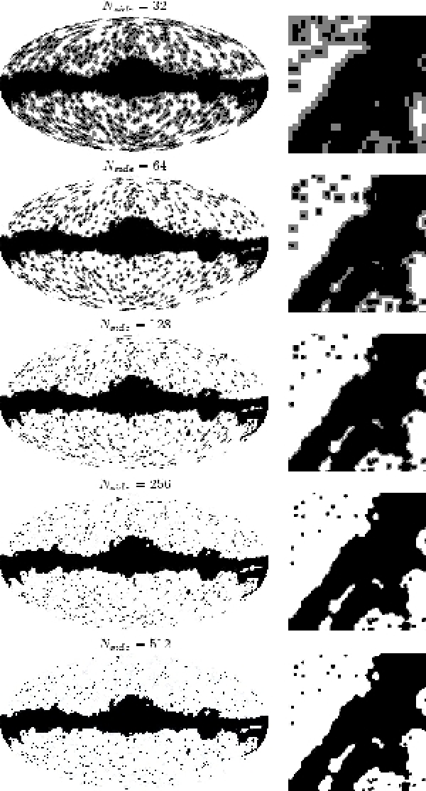
Figure 1: These are the 5 masks used for the one-point correlations. Left column is mollweide projection of the sky; right column is HEALPix base tile 6, where the upper left corner is northernmost. Tile 6 is directly opposite the galactic center; it’s solid angle is exactly 1/12 of the full sphere’s. Paranoid mask is black, extended paranoid mask extends it in grey.

III.4 One-Point Multi-Resolution Results

From the cumulative distribution functions (CDFs) in figure 2, one can see how the difference between correlated noise and white noise changes with resolution. The resolution has a dramatic effect on the number of extrema and on their mean value. At lower resolutions, the CDFs for the white noise and correlated noise look very similar, as one would expect.

It is true that switching from white noise to correlated noise reduces our original detection of the hot and cold spots not being hot and cold enough. However, the switch to correlated noise reduces the number of hot and cold spots in the simulations, so now we have too many extrema. Whether or not there are too many extrema also seems to be heavily dependent on the resolution at which we find the extrema.

At all scales, we do find the variance of the extrema to be slightly low.

Because we have only 110 correlated noise samples, we cannot claim any 95% fluctuations for this noise model. We can claim occasional 95% fluctuations for the 800 white noise samples we have, but in light of the dramatic differences between the CDFs, unlikely statistics from the white noise simulations are more likely to be indications of an incorrect noise model than of non-Gaussianity. Nonetheless, we do calculate where 95% fluctuations occur and mark them in figure 3.

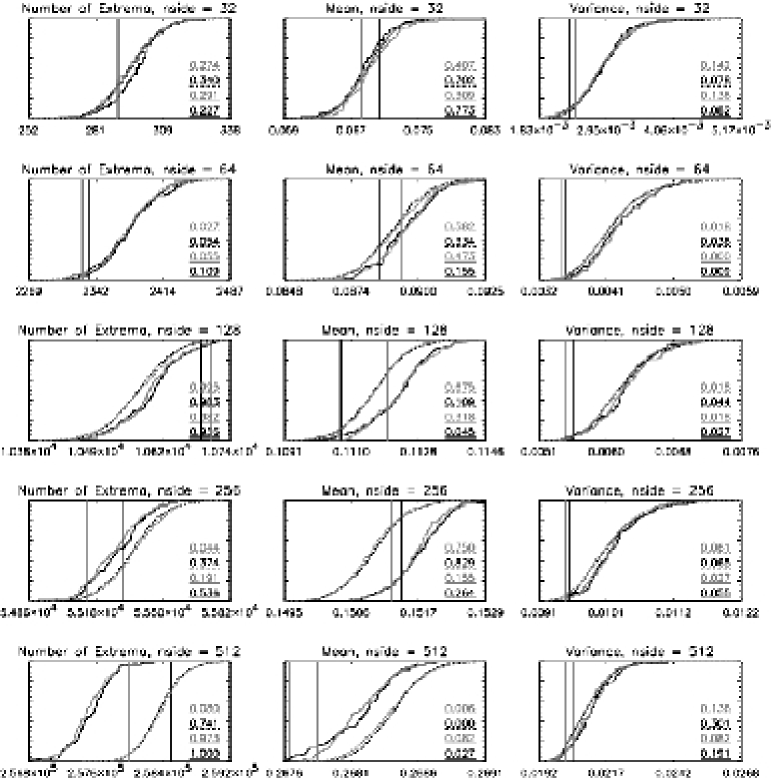
Figure 2: Cumulative distribution functions of the hot and cold spot statistics from various simulations. The grey (black) dashed line is the CDF for the hot (cold) spots from the 800 white noise simulations. The grey (black) solid line is the hot (cold) spot CDF from the 110 correlated noise simulations. The vertical grey (black) line gives the location of the WMAP statistic for the hot (cold) spots. Estimates $\hat{p}$ of the probability of a simulation’s statistic falling below the WMAP statistic are printed on the graph and underlined with the appropriate line. All simulations use the best fit power spectrum, the kp0 mask (degrading is detailed in the paper), and data from the W band. Units for the mean statistics are $mK$ and units for the variance are $mK^{2}$.

	Number		Mean		Variance		Skewness		Kurtosis
	white	corr.	white	corr.	white	corr.	white	corr.	white	corr.
32, max	0.274	0.291	0.407	0.309	0.142	0.136	0.391	0.427	0.114	0.118
32, min	0.340	0.227	0.702	0.773	0.078	0.082	0.928	0.927	0.161	0.136
64, max	0.027	0.055	0.582	0.473	0.018	0.000	0.390	0.482	0.940	0.964
64, min	0.054	0.109	0.334	0.155	0.036	0.009	0.887	0.827	0.441	0.491
128, max	0.995*	0.982	0.675	0.318	0.018	0.018	0.141	0.100	0.990*	0.973
128, min	0.983	0.936	0.109	0.045	0.044	0.027	0.794	0.800	0.950	0.936
256, max	0.044	0.191	0.750	0.155	0.061	0.027	0.610	0.591	0.900	0.900
256, min	0.374	0.536	0.829	0.264	0.065	0.055	0.822	0.745	0.683	0.709
512, max	0.080	0.973	0.006*	0.082	0.136	0.082	0.426	0.527	0.385	0.445
512, min	0.741	1.000	0.000*	0.027	0.301	0.191	0.853	0.845	0.627	0.682

Figure 3: Estimates $\hat{p}$ of the probability $p$ that a simulation statistic will be lower than the WMAP statistic. Column headings signify the statistic and whether the noise was white or correlated in the simulations. For this table, we used 110 correlated noise simulations and 800 white noise simulations. Rows labels signify the value of $N_{side}$ and whether the statistics are for maxima or minima. Values of $\hat{p}$ that are significant for our 95% level test have asterisks. Only the white noise has enough simulations to enable a 95% detection. The first 6 columns of data are presented graphically in figure 2.

III.5 Varying the Amplitude of the Noise

We also check the effect of varying the amplitude of the noise. The WMAP team quotes an uncertainty of the noise amplitude of 0.06% (at one standard deviation) HinshawBarnes03 . When including this in our analysis of the mean of the extrema, we find that the WMAP mean statistics are still qualitatively low, but our results are very sensitive to this value. The numerical results are given in figure 4 and plots of the CDF functions are shown in figure 5.

Again, with only 110 samples, our statistics are not strong enough to claim a 95% fluctuation. In some cases, it is clear that more samples will not help. For example, three simulations out of 110 have more cold spots than the WMAP data, at $N_{side}=512$. The number of cold spots in the WMAP data will not likely be a three sigma fluctuation; it will probably be just under two sigma. For the hot spots, however, all of the simulations have fewer maxima than the WMAP data. In this case, more correlated noise simulations would be useful to determine the significance of this result.

Use of the correlated noise has two effects. It makes the fluctuation in the mean statistic much less significant (if we also allow a one sigma shift in the noise amplitude). Secondly, it indicates that there are too many extrema in the WMAP measured CMB, a result not seen in the white noise. This second effect is not affected by our shifts in the amplitude of the noise.

statistic	$-3\sigma$	$-2\sigma$	$-1\sigma$	$0\sigma$	$1\sigma$	$2\sigma$	$3\sigma$
Number of Local Extrema max	0.991	1.000	0.982	0.991	0.991	0.982	0.982
Number of Local Extrema min	1.000	1.000	1.000	1.000	1.000	1.000	1.000
Mean max	0.782	0.509	0.255	0.109	0.027	0.000	0.000
Mean min	0.345	0.155	0.064	0.009	0.000	0.000	0.000
Variance max	0.145	0.136	0.127	0.091	0.055	0.127	0.091
Variance min	0.291	0.273	0.191	0.227	0.245	0.209	0.200
Skewness max	0.455	0.509	0.464	0.473	0.373	0.455	0.409
Skewness min	0.873	0.909	0.864	0.927	0.900	0.827	0.882
Kurtosis max	0.373	0.355	0.382	0.464	0.409	0.464	0.355
Kurtosis min	0.718	0.682	0.727	0.709	0.673	0.618	0.691

Figure 4: Number of standard deviations by which the amplitude of the correlated noise was shifted. Hinshaw et al. HinshawBarnes03 cite the error in the noise amplitude to be 0.06%, so $-3\sigma$ corresponds to multiplying the amplitude by exactly 0.9982, and $3\sigma$ corresponds to multiplying by exactly 1.0018, etc. This multiplication is carried out after the proper scaling of the correlated noise, discussed in section III.2. The data for the first two statistics is presented graphically in figure 5.

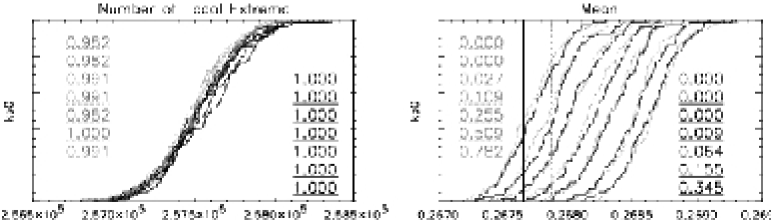
Figure 5: This figure shows the cumulative distribution functions for the statistics generated by shifting the correlated noise amplitude by $n\sigma$, where $n$ ranges from -3 to 3. 110 correlated noise maps are used. The grey statistics (and dotted lines) are for maxima, the black (and solid lines) for minima. From top to bottom, the numbers are values of $\hat{p}$ for $n=3$ to $n=-3$. The vertical lines are the WMAP values. Note: Only the Mean statistic (plot on the right) shows the CDFs spread apart from each other; the other 4 statistics have the CDFs on top of each other, as in the left plot. Also, the detection of non-Gaussianity in the mean is weaker when you consider a $-1\sigma$ shift in the correlated noise amplitude. The CDFs would become smoother with more than 110 simulations.

IV Smoothing One- and Two-point Analysis

The process of simulation and data reduction is very similar to the previous one, except that we smooth instead of changing resolution. The smoothing increases the signal to noise ratio and therefore reduces our sensitivity to the noise model. Also, we are free to choose the smoothing scale without being tied to the discrete pixel sizes of the HEALPix scheme. We again describe the simulation and data reduction process.

Our simulation process has only two steps: creating a CMB sky and adding white noise. Again, this is an acceptable approximation of the WMAP data if our final statistics only depend on the accurate characteristics of this approximation. To assure this in our data reduction, we again ignore the monopole and dipole moments, as well as the region contaminated by galactic foregrounds.

To mask the sky and check for large-scale anisotropies in the statistics, we extend the kp0 mask to different hemispheres, as in LW04. This yields four other Galactic masks: Galactic North and South masks (GN, GS) and Ecliptic North and South masks (EN, ES). See figure 7. When masking a CMB map, we set the temperature fluctuations inside the mask to zero to assure that later smoothing does not allow contamination in the masked region to leak out. To remove dependence on the monopole and dipole, we also remove these moments outside of the galactic mask we use.

To remove dependence on the small scale structure of the noise, we smooth the sky, with either a 50 arcminute or 3 degree Full Width at Half Maximum (FWHM) beam. To choose the smoothing scale, we arbitrarily decided to suppress the power by a factor of 10 at the multipole $\ell$ value where the signal to noise has dropped to a ratio of 1. The signal to noise is 1 at about $\ell=350$, so we choose a Gaussian smoothing FWHM scale of 50 arcminutes. As seen in figure 6, this suppresses the CMB power spectrum by a factor very close to 10 at $\ell=350$. We also check our results with 3 degree smoothing scale, where the noise is entirely subdominant.

After the smoothing, we find the maxima and minima. However, the smoothed temperature map and therefore these extrema will be affected by the zeroed pixels inside the mask, so we want to ignore extrema that are significantly affected by the presence of the mask. To do this, we create an adjusted mask. We smooth the original mask (kp0, GS, GN, ES, or EN) with the same FWHM Gaussian beam as we will use to smooth the CMB, and we mask all areas with values less than 0.9. Recall the convention that unmasked pixels have a value of 1 and masked pixels have a value of 0. When we ignore extrema inside this adjusted mask, we ignore most of the extrema which have been significantly affected by being close to a region of zeroed pixels. Our value of 0.9 is less conservative than Eriksen et al. EriksenBanday04 who use 0.99. This value affects how strictly we want to ignore mask effects. It does not affect the significance of our results, because the simulations and the WMAP data are treated identically.

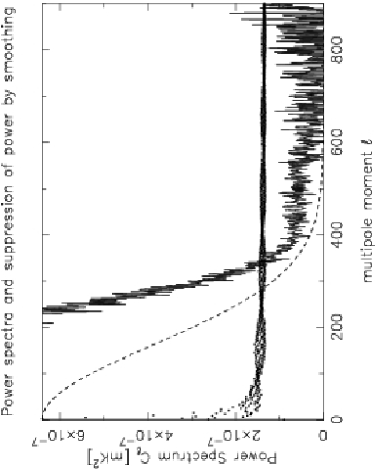
Figure 6: The solid line is the measured temperature-temperature power spectrum from the first year WMAP data. The dots are the average (over 110 simulations) of the W band correlated noise power spectrum. Note the ringing, which is due to the pixelization interacting with the scanning strategy. The dashed line is the unitless suppression of power (due to a 50 arcminute FWHM Gaussian smoothing), which has been rescaled to fit the height of the graph. Note that at $\ell=350$, where signal to noise is about 1, smoothing suppresses power by a factor of about 10.

The process for simulating and and reducing the maps is as follows:

1. Simulate a map with $N_{side}=512$, $\ell_{max}=700$ (or $\ell_{max}=300$, for 3 degree FWHM smoothing), and the WMAP measured power spectrum.

2. Add in white noise, according to the effective number of observations on each pixel.

3. Set the temperature fluctuation to zero inside a galactic mask.

4. Remove the monopole and dipoles outside of that same mask.

5. Smooth with a 50 (or 180) arcminute FWHM Gaussian beam.

6. Find the local extrema.

7. Discard extrema inside the adjusted version of the mask in step 2.

8. Calculate statistics on the extrema for further analysis.

A few images of the various stages of this simulation process are shown in figure 8. We compare these simulations to the WMAP cleaned temperature map data, which goes through the same process, starting at step 3.

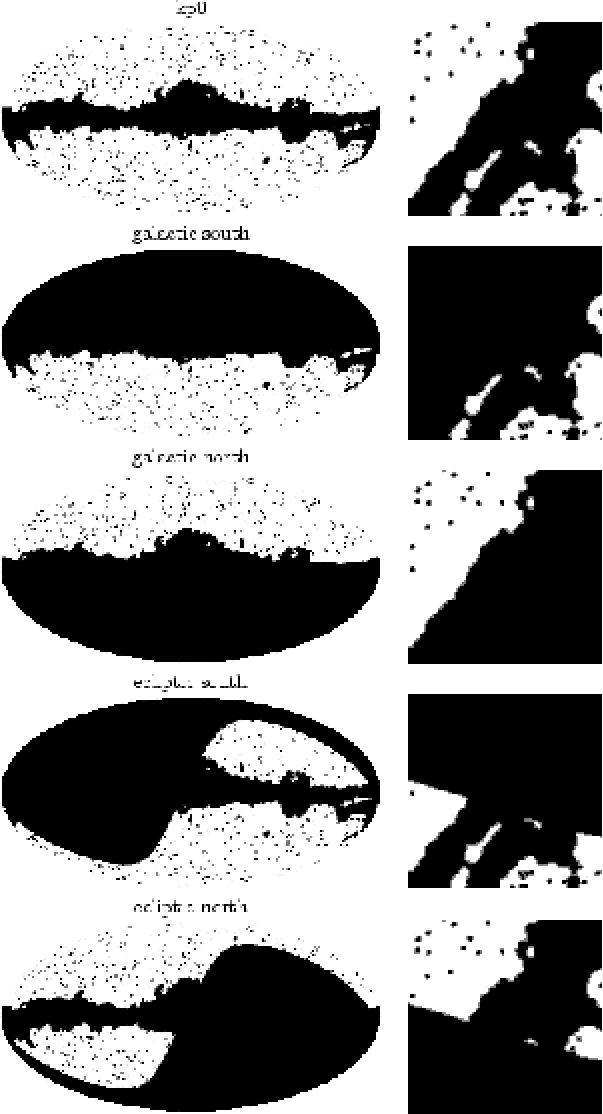
Figure 7: These are the 5 masks used for the two-point correlations. Left column is mollweide projection of the sky; right column is HEALPix base tile 6, where the upper left corner is northernmost. Tile 6 is directly opposite the galactic center. The mask is black, the adjusted mask for 50 arcminute FWHM smoothing includes the mask and the thin grey region extending the mask.

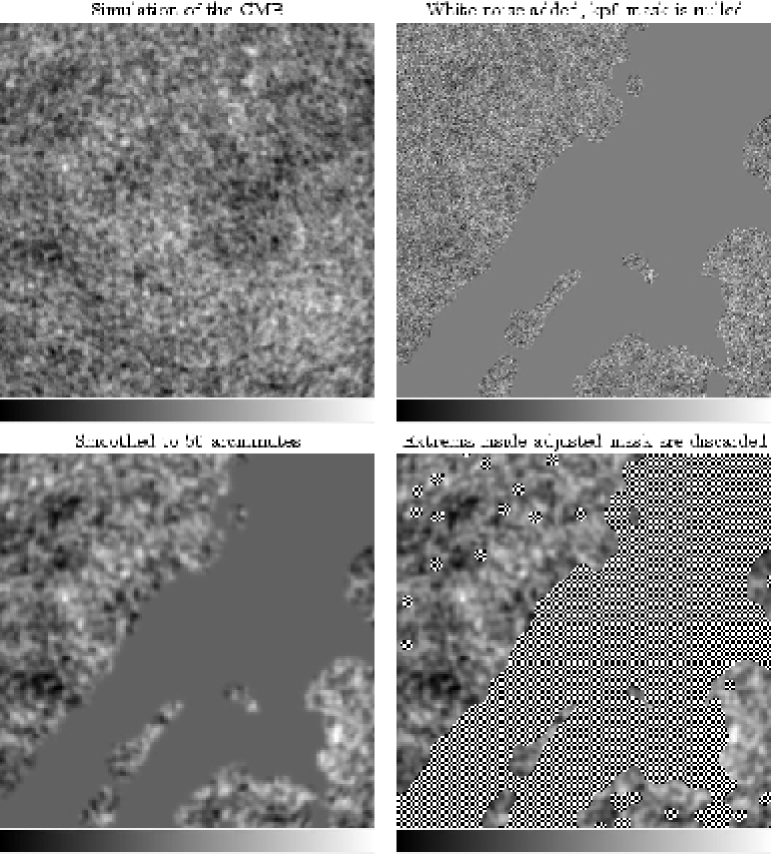
Figure 8: These are images of base tile 6 in the HEALPix scheme at various steps in the simulation process. North is in the upper left. Range of color scale varies between some images.

IV.1 One-Point Statistics

We performed 4000 simulations of Gaussian CMB skies. A 99% detection would require fewer than 10 of the statistics to be below (or above) the WMAP statistic. A 95% detection only requires fewer than 84 of the statistics to be below the WMAP statistic. See the appendix for details.

Some results for the one-point statistics are shown in figure 9. There are no 99% detections, but there are several 95% detections. For the mean statistic, the hot spots do not seem particularly unusual, but the cold spots are too warm in the Galactic North at 50 arcminute smoothing. We also have 95% detections in the Ecliptic North with the hotspots not having enough variance at 50 arcmin smoothing and the cold spots not having enough variance at 3 degree smoothing. With respect to skewness, the cold spots have too much negative skewness at both smoothings. It is possible that this is caused by a single very cold cold spot, perhaps that described by CruzMartinezGonzalez05 . The hot spots have too little skewness at the 3 degree smoothing.

We calculate 100 one-point statistics, and 7 of them give 95% detections, so one could argue that these detections are not highly significant. Nevertheless, it is interesting to see that the detections support previous results, such as the lack of power in the Ecliptic NorthEriksenHansen04 .

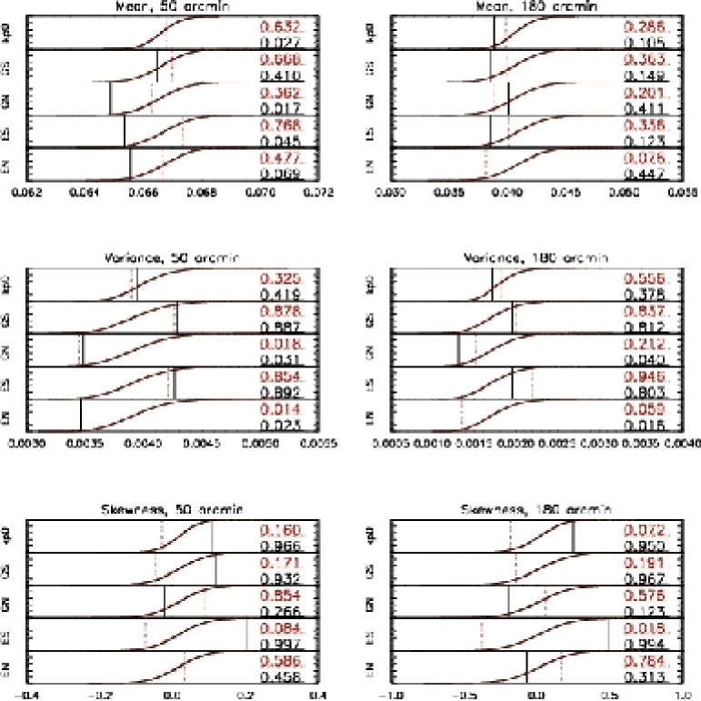
Figure 9: These are cumulative distribution functions of selected one-point statistics for 50 and 180 arcminute smoothing levels. Hot spot (maxima) statistics are in red and are the upper number in each pair. Cold spot statistics are in black. The vertical lines indicate the position of the WMAP statistic. Mean statistics are given in $mK$, variance is in $mK^{2}$, and skewness is dimensionless. The mean and skewness values of the minima have been multiplied by $-1$ before creating CDFs, for easier comparison with the maxima.

IV.2 Two-Point Statistics

IV.2.1 Calculating Two-point Functions

For the two-point functions, we perform two general analyses on the extrema. The first is related to the method used by Heavens and Sheth HeavensSheth99 where they look at the point-point correlation function of the locations of the maxima above a certain threshold (and minima below a threshold). We arbitrarily pick a threshold of $2\sigma$, where $\sigma$ is the standard deviation of all the temperatures in the map outside the (non-adjusted) mask.

The other analysis is where no threshold is applied to the extrema and the two-point statistics of the temperature field at the locations of the extrema are calculated. It has been proposed that this two-point function is very close to the two-point function on the full sphere KashlinskyHernandezMonteagudo01 .

In both analyses, the statistics we calculate are motivated by the concept of a correlation function. We simply find the average number of pairs at a given angular separation, or the average product of spot temperatures at some separation. We calculate three statistics of this form: between maxima and maxima, between minima and minima, and between maxima and minima.

Consider the spot-spot statistics between maxima and minima, for example. We select all pairs with one hot and one cold spot and find the angles between the spots. These angles we bin into 1000 equally spaced bins of angular separation between 0 and $\pi$ radians. To remove dependence on the number of spots, we normalize the histogram we just made by dividing by the total number of counts. This makes the bins sum to 1. Eriksen et al. EriksenNovikov04 have already studied the Minkowski functionals on the CMB, which are related to the number of spots above a threshold, so we did not feel the need to study it further by including information about the number of spots in our data set. The normalized histogram contains the correlation information, but it is slightly dependent on the pixelization and highly dependent on the geometry of the mask we used.

Suppose we wanted to calculate the true underlying correlation function, independent of the geometry of the mask. We do not need to do this in our statistical analysis (and in fact we do not), since we have exactly the same geometric masking effects included in both the WMAP data and simulations. Nonetheless, if we wanted to determine the mask-independent correlation function, we would need to know the effects of the mask. For this purpose, we bin the angles between pairs in a random distribution of “maxima” and “minima” for each CMB simulation. The number of randomly placed extrema is determined by the number of extrema found in that simulation. The underlying correlation function is the excess probability of finding pairs at a given angle. To obtain this for each angular bin, we divide the normalized number of pairs from the CMB simulation by the average normalized number of random pairs in that bin, and subtract 1. This gives us a mask independent correlation function for each iteration, which we can use to visually examine our results.

Calculating the temperature-temperature two-point statistics is very similar to calculating the spot-spot statistics. Instead of counting the number of angles that fall into a given bin, we find the average product of temperatures for pairs of spots in that angular bin. This can also be turned into a correlation function, if only for visual examination.

IV.2.2 Reducing Two-point Functions to a Single Number

Now we must reduce a 1000 dimensional discretized two-point statistic $\xi(\theta)$ into a single statistic, a single real number. We treat $\xi$ as a 1000 dimensional vector. First, we reduce the dimension by ignoring some of the data. We do this in two ways: by re-binning the vector into 40 bins, and by ignoring all but the first 40 of the 1000 bins. After this, we calculate a $\chi^{2}$ value for the lower dimensional $\xi$ vector, based on the covariance $C$ of those vectors. We define $\chi^{2}\equiv\xi^{T}C^{-1}\xi$. Since we must be sure to treat the WMAP two-point vector in the same way as the simulation vectors, and we do not want to include it in the calculation of the covariance matrix, we must use some simulation vectors to define the covariance matrix and calculate our $\chi^{2}$ statistics with the rest. We calculate the covariance matrix $C$ with the first 1000 vectors $\xi$ and then find where the WMAP data lies in the distribution of $\chi^{2}$ values of the rest of the $\xi$ vectors. We also visually check that the distribution of $\chi^{2}$ values from the vectors used to make the covariance is not excessively different from that of the rest of the vectors. This verifies that we are using enough vectors to define $C$.

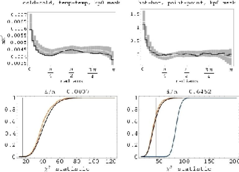
Figure 10: Upper left: temperature-temperature correlation, minima, full sky. Upper right: spot-spot correlation, maxima, full sky. The vertical axis is the excess fractional probability density, for finding a pair of points at a given angular separation. In the correlation functions, the black line is the WMAP data, the white lines are the median simulation values, and the grey band is a $2\sigma$ error band calculated from the simulations. Lower: Cumulative distribution functions for $\chi^{2}$ statistics. They correspond to the upper plots.

IV.3 Two-point results

		7.2 degree		180 degree
		pt-pt	temp-temp	pt-pt	temp-temp
kp0	min	0.14133	0.69100	0.05033	0.00000
kp0	max	0.09400	0.01000	0.38933	0.11567
kp0	cross	0.41833	0.18700	0.01633	0.02067
GS	min	0.03567	0.85800	0.87500	0.16300
GS	max	0.14633	0.10367	0.11533	0.43467
GS	cross	0.90200	0.59900	0.89000	0.80567
GN	min	0.87400	0.28033	0.07767	0.31033
GN	max	0.30600	0.21100	0.49200	0.72667
GN	cross	0.10233	0.06967	0.22933	0.83233
ES	min	0.42667	0.77000	0.73033	0.51933
ES	max	0.11500	0.16633	0.33967	0.65267
ES	cross	0.36467	0.38833	0.54033	0.51900
EN	min	0.21833	0.20033	0.19933	0.20533
EN	max	0.03100	0.07367	0.23033	0.14067
EN	cross	0.23700	0.18700	0.04800	0.12700

Figure 11: These are our estimates $\hat{p}$ of the position of the WMAP two-point statistic among the simulated statistics. These results are for 50 arcminute FWHM smoothing, where 1000 iterations went to create the covariance matrix and position of the WMAP statistic is found among the remaining 3000. The different rows show results for different masks, as well as the minima-minima, maxima-maxima, and minima-maxima statistics. The columns show the results for the nearest 7.2 degrees (first 40 bins) of our two-point statistics, as well as for the full-sky 180 degree two-point statistics. Columns also show the different results for the spot-spot and temperature-temperature statistics. Note the 0 value in the upper right corner.

		7.2 degree		180 degree
		pt-pt	temp-temp	pt-pt	temp-temp
kp0	min	0.75833	0.69500	0.83800	0.18100
kp0	max	0.26333	0.16533	0.62600	0.27000
kp0	cross	0.95433	0.69967	0.83500	0.14833
GS	min	0.40567	0.80267	0.78467	0.42267
GS	max	0.98967	0.88833	0.93700	0.52133
GS	cross	0.00067	0.32900	0.66933	0.75400
GN	min	0.34700	0.11933	0.08233	0.03267
GN	max	0.59533	0.80900	0.17967	0.60667
GN	cross	0.65267	0.73033	0.26500	0.80100
ES	min	0.10300	0.81800	0.84533	0.51967
ES	max	0.62600	0.54967	0.63733	0.84300
ES	cross	0.82933	0.82333	0.45500	0.71167
EN	min	0.67800	0.20933	0.41333	0.17833
EN	max	0.75033	0.73200	0.36067	0.33567
EN	cross	0.69700	0.04600	0.12133	0.17533

Figure 12: This is the same data as figure 11, except for 180 arcminute FWHM smoothing.

Our results here are for 4000 simulations. The first thousand go to define the covariance matrix, so the WMAP statistic is compared to the statistics for the remaining 3000. A 95% detection requires $0\leq\hat{p}\leq 0.02$ or $0.98\leq\hat{p}\leq 1$, and a 99% detection requires $0\leq\hat{p}\leq 0.002$ or $0.998\leq\hat{p}\leq 1$, where $\hat{p}=i/n$ is the same as in our previous paper and is also defined in the appendix.

The most interesting result is in the temperature-temperature correlation function for the kp0 masked full-sky correlation function. For 3000 iterations, the WMAP statistic fell lower than all of them. To better determine the significance of this result, we ran a set of 20,000 simulations for this particular mask. Again, the first 1000 went to determine the covariance matrix. Of the remaining 19,000 simulations, 13 of their statistics fell lower than the WMAP statistic. This is extremely close to a $3\sigma$ detection, it comes to be $2.989\sigma$.

One interesting point about this result is that our $\chi^{2}$ statistic is too low. This means that instead of fitting the distribution of two-point functions too poorly, it instead fits them too well. In fact, it fits the covariance matrix describing the two-point functions better than the two-point functions that went into making that covariance matrix. This is a very unusual result.

It is also curious that we only see this for the kp0 mask and not for the masks in which we cut out half of the sky. This suggests that our effect is different from those that led to recent claims of anisotropy in the CMB.

To check to see if this result is an effect of foregrounds, we repeat our simulations for 3000 iterations in the V-band, just for the kp0 mask. We take 1000 simulations for the covariance matrix, and find the position of the WMAP statistic among the remaining 2000. We find that the min-min temp-temp WMAP statistic on the full sky then falls just above 5% of the simulation statistics. However, we find that if instead of the min-min statistics we look at the min-max (cross), then we find that it now sits lower than all 2000 of the simulation statistics.

V Conclusions

In this paper we present frequentist hypothesis tests to check for non-Gaussianity in the CMB using the one and two-point statistics of hot and cold spots at several angular scales. We use and advocate a robust statistical test that reduces the probability of a false detection of non-Gaussianity to a level commensurate with the significance of the detection.

A Mathematica notebook and small user-friendly C program are available for determining the significance in this robust hypothesis test where a measurement is compared to Monte-Carlo simulations. The method and C code are described in the appendix. The code is available at the web page http://cosmos.astro.uiuc.edu/$\sim$dlarson1/facts/.

While the WMAP hot spots are too cold compared to the white noise simulations, this is no longer as dramatically true when we use the correlated noise simulations. The detection drops to below $2\sigma$. Instead, we find that there are now too many hot and cold spots in the WMAP data. We cannot give this qualitative statement a significance at or above $2\sigma$ because we only have 110 correlated noise simulations. We also find that the variance continues to be qualitatively low.

While the nature of our result is sensitive to changes in the noise model, the significance is not. Allowing the amplitude of the white noise to vary by two standard deviations puts the CDF squarely around the WMAP measurement. This means our result did not go away; we may have error either in the amplitude of the noise or from statistical fluctuations in the CMB, but we still need to move something by two standard deviations to make them match.

When we switch to the properly correlated noise samples, regardless of their amplitude (within three standard deviations) we definitely get too many cold spots, and probably too many hot spots. This was unexpected, since the white noise did not show an unusual number of hot or cold spots.

Our main result comes from our investigation of the two-point statistics. We find an anomaly in the full-sky minima-minima temperature-temperature two-point function using the kp0 mask. This is a very large fluctuation, unlikely at the 3 sigma level. We observe this anomaly only on the full sky. This suggests that our effect is distinct from those that led to recent claims of anisotropy in the CMB.

In addition to this 3-sigma result, we also have several 2-sigma results. For example, we see low variance of the hot spots at 50 arcminute smoothing, the high skewness of the cold spots at both 50 and 180 arcminute smoothings, and a low “$\chi^{2}$” statistic for the point-point function between maxima and minima for the 180 arcminute smoothing (a 2.7 sigma result).

We have demonstrated that there is a statistically highly significant difference between the WMAP data and our Gaussian Monte-Carlo simulations. This can be interpreted in one of three ways: it is just a large fluctuation, it is caused by non-Gaussianity, or it caused by some other unknown foreground or systematic effect that we do not consider in our model of the WMAP data.

Appendix A User’s Guide and Statistical Methods

This appendix contains a brief user’s guide for the facts program in section A.1 and a more detailed explanation of our statistical test in section A.2. In section A.3 we connect our discussion to the derivation of frequentist confidence intervals in LW04, and we close with a brief conceptual comment on tests of non-Gaussianity in section A.4.

A.1 Users Guide for facts

To aid in the calculation of significance, we provide a publicly available code written in c. It is named facts, which stands for a Frequentist’s Ally for the Calculation of Test Significance. To compile the code on a typical linux system, unzip and untar the file, enter the facts directory which was created, and type make. This will make the executable facts. The program is small enough that a makefile is not necessary, but I include it for convenience.

The syntax for the command can be retrieved by executing facts without any command line arguments. The program takes from three to five arguments.

facts s n i [alpha [beta]]

• s: this value is either 1 or 2 for a single or double sided test.

• n: this is the number of simulated statistics calculated.

• i: this is the number of simulated statistics that fell below the test statistic. If i is a negative number, the code prints out information on what values of i will reject the hypothesis.

• alpha: this is a number between 0 and 1 that parameterizes our hypothesis. For a single sided test, the hypothesis is $p\in(\alpha,1]$. For a double sided test, the hypothesis is $p\in(\alpha/2,1-\alpha/2)$. If not specified, the default value is $\alpha=0.05$.

• beta: this is a number between 0 and 1 that gives an upper limit on the probability of a type I error (rejection of the hypothesis when the hypothesis is actually true). If not specified, it takes the value of $\alpha$.

The code takes the values of s, n, $\alpha$, and $\beta$ and constructs a test. If i satisfies that test then the hypothesis is accepted, otherwise it is rejected. The code prints out information whether i satisfies the test, and what the minimum values of $\alpha$ and $\beta$ are for which i will satisfy the test.

A few examples follow. The next command determines whether a two-sided test with a $0.02$ maximum probability of a type I error will accept the hypothesis that $p\in(0.005,0.995)$ when only 17 out of 10000 statistics fell below the test statistic.

facts 2 10000 17 0.01 0.02

The command below determines if 5 out of 1000 statistics falling below the test statistic is few enough to reject the hypothesis $p\in(0.025,0.975)$ when the test has a 5% maximum chance of a type I error.

facts 2 1000 5

While this program is reasonably fast, it is not optimized for pathological requests. It is slower for larger values of n, i, $\alpha$, and $\beta$.

A.2 Statistical Testing

A.2.1 The Problem

The statistical analysis we discuss in this paper can be reduced to the following problem. We are given a few thousand ($=n$) random numbers $\{x_{j}\}$, $j=1\ldots n$ which have come from some random number generator (distribution), with some probability density function (PDF) $f(x)$. We are also given a single number $x_{0}$ and asked to determine if we have any reason to believe, statistically, that it may not have come from that same random number generator.

A.2.2 The Solution

Because this is a statistical problem, we cannot do what we naturally want to do: prove that $x_{0}$ was or was not chosen from the same distribution as the $\{x_{j}\}$. Instead we must settle for a weaker statement about how large a fluctuation $x_{0}$ is, if it were drawn from the distribution of the $\{x_{j}\}$. This appendix describes how to make statistical statements about the size of this fluctuation.

We begin by assuming that the single number $x_{0}$ did come from the random number generator that produced the $\{x_{j}\}$. Given this, we attempt to determine how large a statistical fluctuation $x_{0}$ is. There are several ways to do this. We will use a completely standard (frequentist) hypothesis test. Our hypothesis concerns a parameter, $p$, which describes how large the fluctuation is. We perform a test on a random variable, $i$, whose distribution is affected by $p$, and, based on the results of that test, decide whether or not to accept the hypothesis.

This method is useful if the pdf is sufficiently complex that it is not practical to evaluate it analytically.

A.2.3 The Random Variable and Its Distribution

The method we use requires knowing only how many of the random numbers $x_{j}$ fell below $x_{0}$. Let there be $n$ random numbers and let $i$ of them fall below $x_{0}$. Then $i$ is our random variable, chosen from the binomial distribution $P(i|p,n)$, where

$$P(i|p,n)=\frac{n!}{i!(n-i)!}p^{i}p^{n-i}$$ (2)

and where $p$ gives the position of $x_{0}$ in the PDF $f(x)$:

$$p\equiv\int_{-\infty}^{x_{0}}f(x)\;dx$$ (3)

We can estimate $p$ with $\hat{p}=i/n$, which is a maximum likelihood and unbiased estimator.

A.2.4 The Hypothesis

Our hypothesis concerns the value of $p$. As previously stated, we would prefer to pick “$x_{0}$ was chosen from the same distribution as the $\{x_{j}\}$ values” as our hypothesis. Since the negation of this hypothesis is extremely difficult to work with, we choose a simpler hypothesis, about $p$:

$$H_{0}:\qquad p\in(\alpha/2,1-\alpha/2)$$ (4)

where $\alpha$ is much less than $1$. Here we use a double sided hypothesis for our test; the case of a single-sided test is discussed in section A.2.6. To a frequentist, the hypothesis $H_{0}$ is either true or false, so it either has a probability of 1 or 0. The statistical test described in this appendix will then be useful to decide whether to accept or reject the hypothesis. The frequentist statement is that “$H_{0}$ is true in a fraction $1-\alpha$ of all possible Gaussian Universes”.

It is certainly true that we could have chosen our hypothesis to be anything of the form $p\in S$ where the set $S\subset[0,1]$ has total length (or measure) $1-\alpha$. We choose $S=(\alpha/2,1-\alpha/2)$ because of our natural inclination to think that values of $p$ far out in the tails of the distribution are unusual. Also, if we had reason to believe that $x_{0}$ were drawn from a distribution whose mean was many standard deviations away from the distribution of the $\{x_{j}\}$, our hypothesis would be a powerful test of whether $x_{0}$ was drawn from the same distribution as the $\{x_{j}\}$.

A.2.5 The Test and Types of Error

Our test must be of the form where we accept $H_{0}$ for certain values of $i$, $i\in I$, and reject it for all others, $i\in\overline{I}$. Here, $I$ and $\overline{I}$ are disjoint and $I\cup\overline{I}=\{0,1,2,\ldots,n\}$. With a statistical test of this form, one is interested in the errors of type I (rejection of a true hypothesis) and type II (acceptance of false hypothesis). I will call their probabilities $\beta$ and $\gamma$, respectively.

	test accepts $H_{0}$,	test rejects $H_{0}$,
	$i\in I$	$i\in\overline{I}$
$H_{0}$ is true	$1-\beta$	$\beta$
$H_{0}$ is false	$\gamma$	$1-\gamma$

Explicit calculation of these probabilities requires us to specify a test. Our test is similar in form to that of our hypothesis. We accept $H_{0}$ whenever

$$i\in\{i_{0}+1,i_{0}+2\ldots,n-i_{0}-1\}$$ (5)

for some specified value of $i_{0}$. Since calculation of $\beta$ and $\gamma$ requires knowledge of $n$, $p$, and the test used, $\beta$ and $\gamma$ are functions of these three values.

$$\beta=\beta(i_{0},p,n)\qquad\gamma=\gamma(i_{0},p,n)$$ (6)

It is desirable to adjust the test (the value of $i_{0}$) so that $\beta$ and $\gamma$ are as small as possible for all values of $p$. Unfortunately, these cannot both be made small. The probability of the test accepting $H_{0}$ must vary continuously as $p$ varies continuously from the region from where $H_{0}$ is true to where it is false. This means that $\beta(i_{0},p,n)=1-\gamma(i_{0},p,n)$ at $p=\alpha/2$ and $p=1-\alpha/2$. We must decide which we want to be small. For this paper, we choose to make $\beta$ small. This all but eliminates the possibility of rejecting $H_{0}$ when it is actually true. As a trade-off, we have the problem of accepting $H_{0}$ when it may be false.

We can construct an explicit expression for $\beta$:

$$\beta(i_{0},p,n)=\sum_{i=0}^{i_{0}}P(i|p,n)+\sum_{i=n-i_{0}}^{n}P(i|p,n)$$ (7)

We want to limit $\beta(i_{0},p,n)$ for any value of $p$ satisfying $H_{0}$, which means we want to limit $\beta(i_{0},\alpha/2,n)$. There are two approaches to this: to fix the hypothesis ($\alpha$) and change the test ($i_{0}$), or to fix the test and change the hypothesis. Suppose we are given the hypothesis and want to determine a test that keeps $\beta$ below some bound. This requires one to progressively increase $i_{0}$ while checking that $\beta(i_{0},\alpha/2,n)$ remains below the desired bound. Alternatively, if we have done our experiment and want to determine the highest possible significance we can assign to it, then we know $i_{0}$ and want to find $\alpha$. Specifically, we set $i_{0}$ to our measured value of $i$, and find the smallest value of $\alpha$ such that $\beta$ is still below some desired bound. For simplicity, we could set $\alpha=\beta$, since we want both values to be low for a highly significant result, and numerically solve for $\alpha$:

$$\beta(i_{0},\alpha/2,n)=\alpha$$ (8)

We can then claim that our test has rejected the hypothesis, and has a probability of a type I error (rejecting a true hypothesis) of $\alpha=\beta$.

For computational purposes, it is useful to note that one of the sums in equation 7 will contribute very little to the value of $\beta$. Let us consider the contribution of the second sum, when it is the smaller of the two. Its maximum value (while still being smaller) occurs when $p=1/2$. We will also estimate the integer $i_{0}+1\approx n\alpha/2$. The value of $i_{0}+1$ will typically be lower than this.

$$\sum_{i=n-i_{0}}^{n}P(i|\alpha/2,n) < (i_{0}+1)P(n-i_{0}|\alpha/2,n)$$ (9)

$$< (i_{0}+1)n^{i_{0}+1}(1/2)^{n}$$

$$\lesssim (n\alpha/2)n^{n\alpha/2}(1/2)^{n}$$

$$\lesssim \exp\{\ln(n\alpha/2)+(n\alpha/2)\ln(n)$$

$$+n\ln(1/2)\}$$

We want this to remain small. To assure that the $\alpha n\ln n$ term does not become larger than the $n\ln(1/2)$ term as $n$ increases, we must have $\alpha\leq k/\ln(n)$ for some $k$. Now we can check the contribution of the second sum (equation 7) to $\beta$ for some reasonable bounds:

$$\alpha\leq 1/\ln n\qquad n\geq 100\qquad i_{0}\leq\alpha n/2.$$ (10)

We find the value of the second sum in equation 7 to be well below $10^{-40}$ whenever these conditions are satisfied. Since the probabilities we test are all much higher than $10^{-40}$, it is safe to ignore the second sum in equation 7 when $\hat{p}\ll 1/2$. By symmetry, it is safe to ignore the first sum when $\hat{p}\gg 1/2$. The facts code makes use of this information by ignoring the second sum and mapping its input to a problem where only the first sum is important.

A.2.6 The Case of a One-Sided Test

It may be useful for other applications to do a one-sided analysis, for example if one will only consider a statistic $x_{0}$ to be unusual if it is lower than most simulated statistics. Our work can be repeated for that case:

$$H_{0}:\qquad p\in(\alpha,1]$$ (11)

We accept the hypothesis when $i>i_{0}$.

$$\beta(i_{0},p,n)=\sum_{i=0}^{i_{0}}P(i|p,n)$$ (12)

To specify a test, we require $i_{0}$ to be small enough that the maximum value of $\beta$, which is $\beta(i_{0},\alpha,n)$, is below some bound. Alternatively, to find the significance of previously obtained results, we set $i_{0}$ to be our measured value of $i$, set $\alpha=\beta$, and solve

$$\beta(i_{0},\alpha,n)=\alpha$$ (13)

to find the maximum significance of our test. As in the double sided case, we can claim that our test rejects the hypothesis $H_{0}$, and our test has a probability of a type I error (rejecting a true hypothesis) of $\alpha=\beta$. The analysis for a single sided confidence interval $H_{0}:p\in[0,1-\alpha)$ can be mapped by symmetry to the above problem.

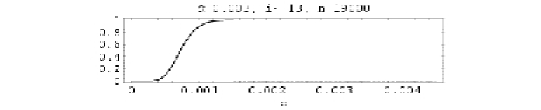
Figure 13: This figure plots $\gamma$, the probability of a false acceptance of the hypothesis (solid), and $\beta$, the probability of a false rejection (dashed), as a function of $p$, for $\alpha=0.003$, $i_{0}=13$, $n=19000$. In order to keep $\beta$ below $\alpha$, we find that $\gamma$ becomes quite large for some values of $p$. In order to avoid false rejections of the hypothesis, we must allow false acceptances sometimes. The region in which $\gamma$ is large becomes smaller as $n$ increases.

A.3 Connecting to Frequentist Confidence Intervals

For an understanding of our statistical test that is sufficient to do calculations, the previous section is enough, and the practical reader can stop here. For the enthusiastic reader, we describe in this section how our test can also be derived using frequentist confidence intervals. This connects the preceding discussion to our alternative derivation for the calculations in LW04.

We use the same formalism in the previous section. There are $n$ simulated statistics, $\{x_{j}\}$. Exactly $i$ of these fall below the test statistic $x_{0}$. The true probability of another simulated statistic falling below the test statistic is $p$, which can be estimated by $\hat{p}=i/n$.

We construct an interval $[p^{-},p^{+}]$ such that the true value of $p$ will be inside the interval at least a fraction $1-\beta$ of the time. Note that this doesn’t mean we think the probability of $p\in[p^{-},p^{+}]$ is at least $1-\beta$ for the specific interval we construct, since $p$ is not a random variable. For some given interval, $[p^{-},p^{+}]$, either $P(p\in[p^{-},p^{+}])=0$ or $P(p\in[p^{-},p^{+}])=1$, and we do not know which is correct. Instead it is helpful to think about many sets of numbers $\{x_{j}\}$ and the same $x_{0}$. Each set will have $n$ numbers, where $i_{k}$ of them fall below $x_{0}$. We construct $\hat{p}_{k}=i_{k}/n$ as before. For each set we also construct the interval $[p^{-}_{k},p^{+}_{k}]$. When we say the probability $P(p\in[p^{-},p^{+}])\geq 1-\beta$, this is to be interpreted with $p^{-}$ and $p^{+}$ as the random variables, since they are both functions of the random variable $i_{k}$. It is a statement about whether the interval falls around the true value of $p$ and not about whether $p$ falls in the interval.

The procedure for constructing this interval $[p^{-},p^{+}]$ is detailed in chapter 20 of Kendall & Stuart KendallStuart73 . We state a few relevant results here.

We define a cumulative distribution function over the index $i$ and a reverse cumulative distribution function as follows:

$$\mathrm{cdf}(i,p,n)=\sum_{j=0}^{i}P(j|p,n)$$ (14)

$$\mathrm{rcdf}(i,p,n)=\sum_{j=i}^{n}P(j|p,n)$$ (15)

From here, we can pick a significance $1-\beta$ for our test and then define $p^{-}=p^{-}(i,n,\beta)$ and $p^{+}=p^{+}(i,n,\beta)$ by

$$\mathrm{cdf}(i,p^{+},n) = \beta/2$$ (16)

$$\mathrm{rcdf}(i,p^{-},n) = \beta/2$$ (17)

Note that here we have constructed a double sided confidence interval. If we wanted a single sided interval, for example $p\in[0,p^{+}]$ with probability $\geq 1-\beta$, then we would have $p^{+}=p^{+}(i,n,\beta)$ defined by

$$\mathrm{cdf}(i,p^{+},n)=\beta$$ (18)

We will not prove this in mathematical detail, but we will restate an argument given by KendallStuart73 for the double sided confidence intervals.

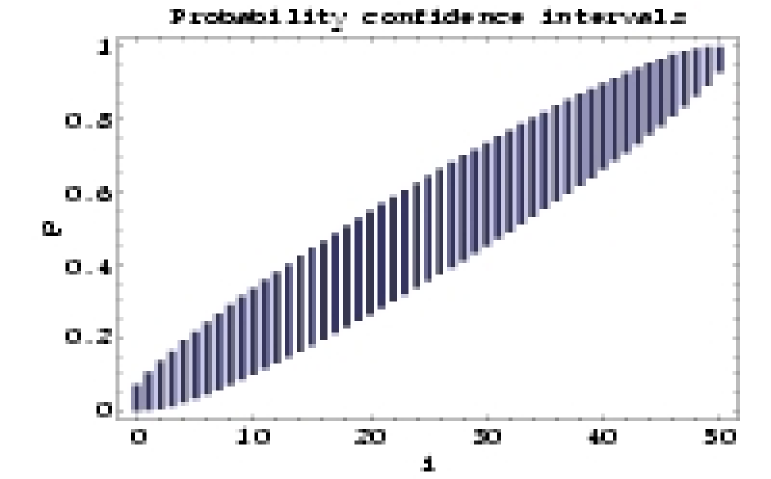
Figure 14: Double sided confidence intervals, $\alpha=0.05$, for all values of $i$ from 0 to $n=50$.

As KendallStuart73 describes, figure 14 can be constructed horizontally and read off vertically. We construct it by fixing $p$ and varying $i$ (as we sum cdf() and rcdf()) while we read off the numbers $p^{-}$ and $p^{+}$ at fixed $i$.

Consider a single value of $p$. Then look across at the values of $i$ that are marked in blue at that $p$ value. By construction, they have probabilities that sum to $\geq 1-\beta$. Hence for any $p$ value, the probability of being in the blue band is $\geq 1-\beta$. But one is in the blue band if and only if $p\in[p^{-},p^{+}]$. Hence the interval $[p^{-},p^{+}]$ will fall around the correct value of $p$ with probability $\geq 1-\beta$. I’ll rephrase it once again: At any specific $p$ value, values of $i$ that cause the interval $[p^{-},p^{+}]$ to surround $p$ will be chosen at least $1-\beta$ of the time.

This frequentist confidence interval can now be used to construct a test of our hypothesis, $H_{0}$: $p\in(\alpha/2,1-\alpha/2)$. We reject the hypothesis if and only if our interval $[p^{-},p^{+}]$ is entirely outside of the interval $(\alpha/2,1-\alpha/2)$. In LW04, we required a double sided confidence interval $[p^{-},p^{+}]$ to be outside of $(\alpha/2,1-\alpha/2)$. This was too conservative, since we only needed a single sided confidence interval to be outside of $(\alpha/2,1-\alpha/2)$. That is, for low values of $\hat{p}$, we reject $H_{0}$ if $[0,p^{+}]$ is completely below the interval ($\alpha/2,1-\alpha/2)$, which means $p^{+}<\alpha/2$. For high values of $\hat{p}$, we reject $H_{0}$ if $[p^{-},1]$ is completely above the interval ($\alpha/2,1-\alpha/2)$, which means $1-\alpha/2<p^{-}$.

This is equivalent to the test previously discussed, as long as the reasonable assumptions in equation 10 hold so that one of the sums in equation 7 can be dropped.

A.4 The Next Step

We can now quantify how large a statistical fluctuation the number $x_{0}$ is among the random numbers $\{x_{j}\}$. Given the number of statistics that fell below the test statistic, we can test the hypothesis that $x_{0}$ is not in the tails (which have total probability $\alpha$) of the distribution. If our test says that $x_{0}$ is indeed far out in the tails of the distribution, then we can decide not to believe that $x_{0}$ came from the same random number generator as the $\{x_{j}\}$. This is in fact the route taken in our paper.

A general caveat of any blind search for anomalies is that one cannot distinguish between a large statistical fluctuation and a genuinely different parent distribution. This is often casually referred to as the “non-dog” problem of non-Gaussianity searches, since the class of things which are not dogs is as large and as difficult to deal with as the class of CMB models which are not Gaussian. The difficulty lies in defining something by negation.

To illustrate this idea, suppose we find a detection for some very small value of $\alpha$. Claiming that $x_{0}$ was not produced by the original random number generator (RNG) is a dangerous thing to do without specifying exactly what random number generator did produce $x_{0}$. Consider, for example, that the $\{x_{j}\}$ are Gaussian distributed with zero mean and unit variance, and $x_{0}=10$. If the only alternative RNG is one which also has zero mean, but has a variance of $10^{-100}$, then what we had originally claimed as evidence against the original RNG would now be considered strong evidence for it.

The ambiguity made apparent in this example holds true generally for any blind test of non-Gaussianity and is not just a feature of our work. Consequently, we must either come up with an alternative model to Gaussianity, or leave the interpretation to the reader.

References

- [1] C. L. Bennett, M. Halpern, G. Hinshaw, N. Jarosik, A. Kogut, M. Limon, S. S. Meyer, L. Page, D. N. Spergel, G. S. Tucker, E. Wollack, E. L. Wright, C. Barnes, M. R. Greason, R. S. Hill, E. Komatsu, M. R. Nolta, N. Odegard, H. V. Peirs, L. Verde, and J. L. Weiland. First year wilkinson microwave anisotropy probe (wmap) observations: Preliminary maps and basic results. ApJS, 148:1, 2003.
- [2] David L. Larson and Benjamin D. Wandelt. The hot and cold spots in the wilkinson microwave anisotropy probe data are not hot and cold enough. ApJL, 613:L85–L88, 2004.
- [3] P. Vielva, E. Martínez-González, R. B. Barreiro, J. L. Sanz, and L. Cayón. Detection of the non-gaussianity in the wmap 1-year data using spherical wavelets. astro-ph/0310273, 2003.
- [4] Xin Liu and Shuang Nan Zhang. Non-gaussianity due to possible residual foreground signalsin wmap 1st-year data using spherical wavelet approaches. astro-ph/0504589, April 2005.
- [5] J. D. McEwen, M. P. Hobson, A. N. Lasenby, and D. J. Mortlock. A high-significance detection of non-gaussianity in the wmap 1-year data using directional spherical wavelets. astro-ph/0406604, February 2005.
- [6] L.-Y. Chiang, P. D. Naselsky, O. V. Verkhodanov, and M. J. Way. Non-gaussianity of the derived maps from the first-year wilkinson microwave anisotropy probe data. ApJL, 590:L65, 2003.
- [7] Lung-Yih Chiang, Peter Coles, and Pavel Naselsky. Return mapping of phases and the analysis of the gravitational clustering hierarchy. MNRAS, 337:488–494, 2002.
- [8] Lung-Yih Chiang, Pavel Naselsky, and Peter Coles. The robustness of phase mapping as a non-gaussianity test. ApJL, 602:L1, 2004.
- [9] C. Park. Non-Gaussian signatures in the temperature fluctuation observed by the Wilkinson Microwave Anisotropy Probe. MNRAS, 349:313–320, March 2004.
- [10] Hans K. Eriksen, Frode K. Hansen, A. J. Banday, K. M. Góroski, and P. B. Lilje. Asymmetries in the cmb anisotropy field. ApJ, 605:14–20, 2004.
- [11] A.M. Aliaga, E. Martinez-Gonzalez, L. Cayon, F. Argueso, J.L. Sanz, R.B. Barreiro, and J.E. Gallegos. Tests of gaussianity. astro-ph/0310706, 2003. Proceedings of “The Cosmic Microwave Background and its Polarization”, New Astronomy Reviews, (eds. S. Hanany and K.A. Olive), in press.
- [12] Paolo Cabella, Frode Hansen, Domenico Marinucci, Daniele Pagano, and Nicola Vittorio. Search for non-gaussianity in pixel, harmonic and wavelet space: compared and combined. astro-ph/0401307, 2004.
- [13] P. Cabella, M. Liguori, F. K. Hansen, D. Marinucci, S. Matarrese, L. Moscardini, and N. Vittorio. Primordial non-gaussianity: local curvature method and statistical significance of constraints on f_nl from wmap data. astro-ph/0406026, January 2005.
- [14] E. Komatsu, A. Kogut, M. R. Nolta, C. L. Bennett, M. Halpern, G. Hinshaw, N. Jarosik, M. Limon, S. S. Meyer, L. Page, D. N. Spergel, G. S. Tucker, L. Verde, E. Wollack, and E. L. Wright. First year wilkinson microwave anisotropy probe (wmap) observations: Tests of gaussianity. ApJS, 148:119–134, 2003.
- [15] Eiichiro Komatsu, David N. Spergel, and Benjamin D. Wandelt. Measuring primordial non-gaussianity in the cosmic microwave background. astro-ph/0305189, 2003.
- [16] Daniel Babich. Optimal estimation of non-gaussianity. astro-ph/0503375, March 2005.
- [17] E. Gaztañaga, J. Wagg, T. Multamäki, A. Montaña, and D. H. Hughes. Two-point anisotropies in wmap and the cosmic quadrupole. MNRAS, 346:47–57, 2003.
- [18] E. Gaztañaga and J. Wagg. Three-point temperature anisotropies in wmap: Limits on cmb non-gaussianities and nonlinearities. PRD, 68:021302, 2003.
- [19] G. Hinshaw, C. Barnes, C. L. Bennett, M. Greason, M. Halpern, R. S. Hill, N. Jarosik, A. Kogut, M. Limon, S. S. Meyer, N. Odegard, L. Page, D. N. Spergel, G. S. Tucker, J. Weiland, E. Wollack, and E. L. Wright. First year wilkinson microwave anisotropy probe (wmap) observations: Data processing methods and systematic errors limits. ApJS, 148:63, 2003.
- [20] NASA. Lambda. http://lambda.gsfc.nasa.gov/, 2003.
- [21] Gary Hinshaw. Private communication, May 2004.
- [22] H. K. Eriksen, A. J. Banday, K. M. Gorski, and P. B. Lilje. The n-point correlation functions of the first-year wilkinson microwave anisotropy probe sky maps. astro-ph/0407271, 2004.
- [23] M. Cruz, E. Martínez-González, P. Vielva, and L. Cayón. Detection of a non-Gaussian spot in WMAP. MNRAS, 356:29–40, January 2005.
- [24] A. F. Heavens and R. K. Sheth. The correlation of peaks in the microwave background. MNRAS, 310:1062–1070, 1999.
- [25] A. Kashlinsky, C. Hernández-Monteagudo, and F. Atrio-Barandela. Determining cosmic microwave background structure from its peak distribution. ApJ, 557:L1, 2001.
- [26] H. K. Eriksen, D. I. Novikov, P. B. Lilje, A. J. Banday, and K. M. Górski. Testing for non-gaussianity in the wmap data: Minkowski functionals and the length of the skeleton. astro-ph/0401276, 2004.
- [27] K. M. Górski, E. Hivon, and B. D. Wandelt. Analysis issues for large cmb data sets. In A. J. Banday, R. K. Sheth, and L. N. Da Costa, editors, Evolution of Large Scale Structure : from Recombination to Garching : Proceedings of the MPA-ESO Cosmology Conference, pages 37–42, Garching, Germany, 1999. PrintPartners Ipskamp.
- [28] M. G. Kendall and A. Stuart. The Advanced Theory of Statistics: Inference and Relationship, volume 2. Hafner, New York, third edition, 1973.