Detection of Cosmic Magnification with the Sloan Digital Sky Survey

Abstract

We present an 8$\sigma$ detection of cosmic magnification measured by the variation of quasar density due to gravitational lensing by foreground large scale structure. To make this measurement we used 3800 square degrees of photometric observations from the Sloan Digital Sky Survey (SDSS) containing $\sim 200,000$ quasars and 13 million galaxies. Our measurement of the galaxy-quasar cross-correlation function exhibits the amplitude, angular dependence and change in sign as a function of the slope of the observed quasar number counts that is expected from magnification bias due to weak gravitational lensing. We show that observational uncertainties (stellar contamination, Galactic dust extinction, seeing variations and errors in the photometric redshifts) are well controlled and do not significantly affect the lensing signal. By weighting the quasars with the number count slope, we combine the cross-correlation of quasars for our full magnitude range and detect the lensing signal at $>4\sigma$ in all five SDSS filters. Our measurements of cosmic magnification probe scales ranging from $60\,h^{-1}\,$kpc to $10\,h^{-1}\,$Mpc and are in good agreement with theoretical predictions based on the WMAP concordance cosmology. As with galaxy-galaxy lensing, future measurements of cosmic magnification will provide useful constraints on the galaxy-mass power spectrum.

1. Introduction

We expect the large-scale structure seen in the low redshift Universe to gravitationally lens background sources, such as high redshift galaxies and quasars. This lensing effect causes both a magnification and a distortion of these distant sources. The systematic distortion of faint background galaxies by gravitational lensing, the cosmic shear, has now been measured by several groups in the past few years (Van Waerbeke et al. 2000; Bacon et al. 2000; Rhodes et al. 2001; Hoekstra et al. 2002a; Van Waerbeke et al. 2002; Jarvis et al. 2003; Brown et al. 2003; Massey et al. 2004), and has been found to be in remarkable agreement with theoretical predictions based on the Cold Dark Matter model. It has also provided new constraints on cosmological parameters, especially on $\sigma_{8},\Omega_{m}$ and the shape of the dark matter power spectrum (for a review, see Van Waerbeke & Mellier 2003; Refregier 2003; Hoekstra 2003). In addition to shear-shear correlations, the cross-correlation of foreground galaxies with background shear, known as galaxy-galaxy lensing has also been measured (Brainerd, Blandford & Smail 1996; dell’Antonio & Tyson 1996; Griffiths et al. 1996; Hudson et al. 1998; Fischer et al. 2000; Wilson et al. 2001; McKay et al. 2001; Smith et al. 2001; Hoekstra et al. 2003). Recent measurements from the Sloan Digital Sky Survey (SDSS; York et al. 2000) have enabled accurate constraints on galaxy halo profiles or more generally the galaxy-mass correlation (Seljak et al. 2004; Sheldon et al. 2004).

In a similar way, the systematic magnification of background sources near foreground matter over-densities, the cosmic magnification, can be measured and can provide largely independent constraints on cosmological parameters. Gravitational magnification in the weak limit has two effects: First, the flux received from distant sources is increased, resulting in a relatively deeper apparent magnitude limited survey. Second, the solid angle is stretched, diluting the surface density of source images on the sky. The net result of these competing effects is an induced cross-correlation between physically separated populations that depends on how the loss of sources due to dilution is balanced by the gain of sources due to flux magnification. Any type of background source can be used to measure this effect (galaxies, quasars, supernovae, etc.), but in practice, previous investigations have used foreground galaxies and background quasars motivated by the large redshift range probed by quasars and general redshift segregation between these two populations. Despite the apparent elegance of this solution, lensing-induced quasar-galaxy correlations have been a controversial subject for more than a decade. Numerous teams have attempted to measure this effect and have reported detections of changes in the density of background quasars in the vicinity of galaxies. However, as seen by reviewing the literature on this type of measurement, the results have been generally discrepant with each other as well as in disagreement with the expected signal from gravitational lensing.

The first analysis of quasar-galaxy correlations was done by Seldner & Peebles (1979) using a sample of $\sim 400$ quasars and galaxies from the Lick catalog that led to a $3.7\sigma$ detection of an quasar excess on $\sim 20^{\prime}$ scales in the vicinity of galaxies. The first measurements aimed at detecting the expected lensing signal used radio-selected quasar samples; this method yielded numerically larger quasar samples as well as a steeper number count relation to enhance the lensing signal. Fugmann (1990) correlated bright, radio-loud quasars at moderate and high redshifts with galaxies from the Lick catalog and found an excess on a 10^′ scale. Bartelmann & Schneider (1993b) repeated the analysis with 56 $z\geq 0.75$ optically identified quasars from the 1-Jansky catalog and confirmed the previous result. Similar excesses were also found by cross-correlating the 1-Jansky quasar catalog with IRAS galaxies (Bartelmann & Schneider 1994; Bartsch et al. 1997) and diffuse X-ray emission (Bartelmann et al. 1994; Cooray 1999). Rodrigues-Williams & Hogan (1994) found a correlation between optically-selected quasars and Zwicky clusters, but with an amplitude that cannot be reproduced by lensing of simple mass models. Seitz & Schneider (1995) revisited the previous 1-Jansky/IRAS analysis, finding agreement for the intermediate redshift quasars but failing to detect any correlation for the high redshift ones. Wu & Han (1995) repeated the cluster cross-correlation using Abell clusters and found no correlation with the 1-Jansky sources. Using wide-field R-band images, Norman & Impey (1999) detected a correlation with 1-Jansky quasars on scales greater than 10^′. Williams & Irwin (1998) and Norman & Williams (2000) cross-correlated LBQS and 1-Jansky quasars with APM galaxies (Maddox et al. 1990) and claimed significant over-densities on angular scales of the order of one degree.

Using optically selected sources, similarly mixed results have been obtained: by correlating UV-excess quasars and APM galaxies in clusters, Boyle et al. (1988) found a $30\%$ deficit of quasars on scales of 4^′ around galaxies. Croom & Shanks (1999) investigated the lensing explanation but found the amplitude of the signal to be too high. Rodrigues-Williams & Hawkins (1995) used variability-selected quasars and found a correlation with Zwicky clusters that they interpret as induced by lensing. Again, the amplitude of the correlation largely exceeded expected results. Associations between red galaxies from the APM catalog and moderate-redshift quasars were investigated by Benítez & Martínez-González (1995). They reported a $\sim 30\%$ excess of quasars within 2^′ from the galaxies and a signal consistent with zero on larger scales. Ferreras et al. (1997) cross-correlated optically selected bright quasars and galaxies. The amplitude and the redshift dependence of their results was inconsistent with either the lensing or the dust explanation, and they suggested that the quasar selection process suffered from incompleteness. More recently, Myers et al. (2003) investigated correlations between galaxy groups and optically selected quasars from the 2dF survey. They found a $3\sigma$ anti-correlation within 10^′, whose amplitude implies that the velocity dispersion of galaxy groups is of the order of 1000 km s^-1, i.e. much higher than expected. In addition, they have investigated the effects of extinction by dust and found them to be negligible. Finally, Gaztañaga (2003) measured the cross-correlation between photometric galaxies and spectroscopic quasars using only the SDSS EDR (Stoughton et al. 2002). In contrast to Myers et al. (2003) they found a positive cross-correlation of 20% on arcminute scales – two results that might be complementary because they probe quasar samples of different apparent magnitude (see, e.g., Myers et al. 2005), although the amplitude of both measurements was far in excess of the expected lensing signal. Compared to our measurements, the Gaztañaga (2003) analysis was done on earlier reductions of EDR data and an incomplete sample of quasars, both of which may have affected the observed signal (see §3.1 for more details). In addition, the foreground and background samples used appear to have significant redshift overlap, which can lead to a much stronger non-lensing correlation.

Clearly, the scatter in the existing observational results is large, ranging from significant positive correlations to null and negative correlations, as well as a variety of claimed scales for the different detections, from half an arcminute to one degree. In addition, quasar-galaxy correlations have been controversial for many years due to the large discrepancy between the claimed detections and early theoretical estimations (Schneider et al. 1992; Bartelmann 1995; Dolag & Bartelmann 1997; Sanz et al. 1997). Indeed, the observed amplitude of previous magnification results was typically an order of magnitude larger than predicted by theory. Initially, it was not clear whether this problem was due to the observations or the models, as the early formalism describing cosmic magnification used several simplifying assumptions: a linearized magnification and a constant bias for the galaxy-dark matter relation. Improvements have recently been made on the theoretical side, i.e., Ménard et al. (2003) went beyond the linearized magnification approximation by including non-linear corrections to the relation between the magnification and density fluctuations, and then compared their results to numerical simulations. Guimarães et al. (2001) introduced a scale-dependent galaxy bias obtained from measurements of galaxy auto-correlation functions. Jain, Scranton & Sheth (2003) modeled the complex behavior of the galaxy bias using the halo-model approach, and Takada & Hamana (2003) added an estimation of the full non–linear magnification contribution by including the magnification profile of NFW halos (Navarro, Frenk, & White 1997) in the halo-model formalism. Together, these works provide an accurate theoretical framework and show that earlier estimations of the amplitude of the cosmic magnification were underestimated by 20 to 30 %. However, this remains insufficient to reconcile the expected signal with the observed cross-correlations.

In this paper, we present the detection of cosmic magnification using a large, uniform sample of photometrically-selected SDSS galaxies and quasars. Contrary to previous results, we find an excess of bright ($g\lesssim 19$) quasars around galaxies and a deficit of fainter quasars, matching the expected variation with quasar number count slope. In addition, the amplitude of the signal and its angular dependence is, for the first time, in agreement with theoretical predictions. Based on a number of data quality and uniformity tests, we find that this detection is robust against possible sources of systematic error that may have plagued previous measurements and represents a genuine detection of magnification bias. The outline of the present paper is as follows: §2 reviews the basic weak lensing models for the expected signal and §3 describes the galaxy and quasar data sets and cross-correlation estimators. §4 summarizes the results from magnitude-limited quasar samples as well as optimally-weighted measurements using the full quasar sample and compares them to the expected signals derived in §2. Finally, §5 discusses the possible applications for further measurements using the SDSS and future large area surveys.

2. Modeling Magnification Statistics

In this section we briefly describe the formalism of cosmic magnification and introduce the notation that will be used below. Let $\mathrm{n_{0}}(f)\,\mathrm{d}f$ be the number of sources with a flux in the range $[f,f+\mathrm{d}f]$ and $\mathrm{n}(f)\,\mathrm{d}f$ the corresponding number of lensed sources undergoing a magnification $\mu$. We write the unlensed source counts as

$$\mathrm{n_{0}}(f)\,\mathrm{d}f = a_{0}\,f^{-s(f)}\,\mathrm{d}f\,,$$ (1)

where $a_{0}$ is some normalization factor and $s(f)$ is the power-law slope as a function of flux $f$. The magnification effect will enlarge the sky solid angle, thus modifying the source density by a factor $1/\mu$, and at the same time increase their fluxes by a factor $\mu$. These effects act as follows on the number of lensed sources:

$$\mathrm{n}(f)\,\mathrm{d}f = \frac{1}{\mu}\;\mathrm{n_{0}}\,\left(\frac{f}{\mu}\right)\;\frac{\mathrm{d}f}{\mu}$$ (2)

$$= \mu^{-2}\,a_{0}\,\left(\frac{f}{\mu}\right)^{-s(f/\mu)}\,\mathrm{d}f$$

If $s$ does not vary appreciably over the interval $[f,f\mu]$, which is well satisfied if $\mu$ departs only weakly from unity, then

$$\mathrm{n}(f)\,\mathrm{d}f = \mu^{s(f)-2}\,n_{0}(f)\,\mathrm{d}f\,.$$ (3)

Expressing this as a function of magnitude, we recover the form appropriate for a magnitude limited sample (Narayan 1989):

$$\mathrm{N}(m)\,\mathrm{d}m = \mu^{2.5\;s(m)-1}\,\mathrm{N_{0}}(m)\,\mathrm{d}m$$ (4)

$$= \mu^{\alpha(m)-1}\,\mathrm{n_{0}}(m)\,\mathrm{d}m,$$

The final form of the exponent ($\alpha(m)-1$) reflects the two distinct effects of magnification and how they interact to produce the signal observed on the sky: the amplification effect that varies as a function of the quasar magnitude and the dilution effect that is a constant regardless of magnitude. The combination of these two effects is the magnification bias.

In the statistical context, magnification creates correlations between foreground and background populations. In the weak lensing regime, i.e. if the convergence ($\kappa$) and the shear ($\gamma$) are small compared to unity, a first-order Taylor expansion of the magnification gives $\mu\approx 1+2\,\kappa$. Using this approximation, a cross-correlation between magnification and foreground matter overdensities can then be easily computed as a function of the matter power spectrum. The formalism for magnification by large-scale structures was first introduced by Bartelmann (1995). Following the prescription and notation laid out in Jain, Scranton & Sheth (2003), the expected magnification bias signal can be written as

$$w_{\rm GQ}(\theta,m) = 12\pi^{2}\Omega_{M}\,(\alpha(m)-1)\times$$

$$\int\mathrm{d}\chi~{}\mathrm{d}k~{}k\,{\cal K}(k,\theta,\chi)\,P_{gm}(k,\chi)$$

$$= (\alpha(m)-1)\,\times w_{0}(\theta),$$

where $m$ is the magnitude of the sources, $\Omega_{M}$ is the cosmological matter density relative to critical, $\chi$ is the comoving distance, ${\cal K}$ is the lensing kernel, and $P_{gm}(k,\chi)$ is the galaxy-dark matter cross-power spectrum. This formulation separates the expected signal into two pieces: $w_{0}(\theta)$, which contains all of the information about non-linear galaxy biasing and the redshift distributions; and $(\alpha(m)-1)$, which varies only with quasar magnitude and controls the sign of the expected signal. We note in passing that $w_{0}$ is closely related to the tangential shear induced by the galaxy-mass correlation, which is measured in galaxy-galaxy lensing. In practice, one needs to consider quasars over a given magnitude range, in which $\alpha(m)$ may vary. In this case we have:

$$w_{\rm GQ}(\theta) = \langle\alpha-1\rangle\times w_{0}(\theta),$$ (6)

where

$$\langle\alpha-1\rangle=\frac{\int\mathrm{d}m\,\mathrm{N}(m)(\alpha(m)-1)}{\int\mathrm{d}m\,\mathrm{N}(m)}\,.$$ (7)

The lensing kernel ${\cal K}$ in Eq. 2 is primarily a function of the redshift distributions of the galaxies and quasars. As in Jain, Scranton & Sheth (2003), we model the redshift distributions as a combination of power-law and exponential cut-off: $dN/dz\sim z^{a}\exp(-(z/z_{0})^{b})$. The galaxy redshift distribution can be inferred from the luminosity functions measured by the CNOC2 survey (Lin et al. 1999) with the appropriate apparent magnitude limits (see §3). For the quasars, photometric redshifts are computed for each quasar (see §3), along with upper and lower redshift bounds and the probability that the quasar is within that redshift range. To model the redshift distribution for each quasar sample, we assume a flat distribution between the upper and lower redshift bounds for each quasar and weight according to the aforementioned redshift probability. To first order the redshift distributions for all five quasar magnitude cuts are indistinguishable, so we use the same fitted distribution to model each cut, making $\langle\alpha-1\rangle$ the only free parameter separating each magnitude bin. Fitting the redshift distributions to the chosen form, we find:

$$\left(\frac{dN}{dz}\right)_{G} {\sim} z^{1.3}\exp\left[-(z/0.26)^{2.17}\right]$$

$$\left(\frac{dN}{dz}\right)_{Q} {\sim} z^{2.56}\exp\left[-(z/2.02)^{12.76}\right],$$ (8)

where the redshift distribution for the quasars is limited to the range $1<z<2.2$ using photometric redshifts (see §3). Figure 1 shows the raw and fitted redshift distributions.

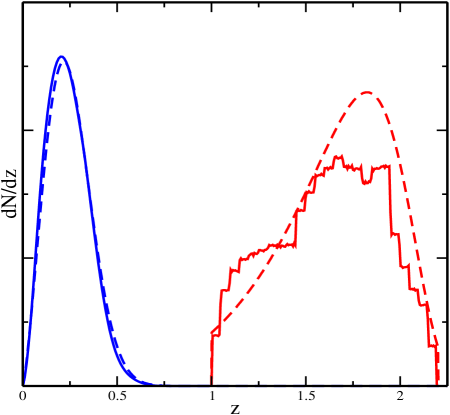
Figure 1.— Galaxy redshift distribution from applying our $17<r<21$ magnitude limit to the CNOC2 luminosity function and quasar redshift distribution inferred from quasar photometric redshifts (solid lines). The fitted redshift distributions from Equation 8 are shown with dashed lines. In all cases, the amplitude scaling is arbitrary.

The only remaining piece of the theoretical calculation is the power spectrum. Since we are in the non-linear regime of gravitational collapse for the smallest angular bins and our foreground redshift distribution is broad, a thorough calculation of the expected signal would involve a matter-galaxy power spectrum calculated with an evolving halo occupation distribution (HOD). However, for the purposes of this paper, we are only interested in checking our measurements against a simple model of the expected signal, leaving the task of extracting the proper HOD behavior for future papers. With that in mind, we assume a simple HOD:

$$\left\langle N\right\rangle(M)=N_{c}+\left(M/M_{0}\right)^{\beta},$$ (9)

where $N_{c}$ is unity for halo mass above $10^{11}h^{-1}M_{\sun}$ and zero otherwise, $M_{0}$ is $10^{12}h^{-1}M_{\sun}$ and $\beta$ is roughly unity. These parameters are approximately what one finds from semi-analytic galaxy codes (cf. Kravtsov et al. 2004) and HOD fits to the SDSS spectroscopic survey 2-point clustering measurements in Zehavi et al. (2004).

We will use this formalism and a flat WMAP cosmology ($\Omega_{M}=0.29$, $\Omega_{\Lambda}=0.71$, $h=0.72$, $n=1$; Spergel et al. 2003) to estimate $w_{0}(\theta)$ and compare our measurements to the theoretical expectations. On small scales, non-linear magnification must be taken into account in order to obtain a more accurate modeling (Ménard et al. 2003; Takada & Hamana 2003), but this level of precision will suffice for our current case. A more detailed modeling which includes marginalization over cosmological and redshift distribution parameters will be used in a future paper in order to constrain some of the model parameters.

With this model in hand, we can test whether the measured signal is due to gravitational lensing in two ways: (i) we can test whether the amplitude of the cross–correlation properly varies as a function of magnitude, i.e. if $w_{\rm GQ}(m)\propto\langle\alpha(m)-1\rangle$, where $\langle\alpha(m)-1\rangle$ is evaluated according to Eq. 7; and (ii) we can check if the angular variation of $w_{\rm GQ}(\theta)$ agrees with theoretical expectations. Showing that the signal satisfies these two conditions is a robust test to demonstrate the lensing origin of the signal and a general lack of systematic contamination.

3. Data Analysis

The use of large, homogeneous samples of galaxies and quasars observed by the SDSS (Gunn et al. 1998; Fukugita et al. 1996; Smith et al. 2002) improves on previous measurements of the cosmic magnification in several key ways. First, the SDSS provides accurate multi-color photometry (Lupton, Gunn & Szalay 1999; Ivezic et al. 2004; Hogg et al. 2001; Pier et al. 2003) over large areas of sky with tight control of the systematic errors that could alter the observed density of sources on the sky (e.g., seeing variations, masks around bright stars, sky background subtraction problems around bright galaxies). Moreover, the accuracy of the photometry is crucial, especially to determine the number of faint sources. If the required photometric accuracy is a few percent, CCD-based photometry is clearly superior to photographic plate data. For example, the 2dF photometric accuracy is approximately 0.2 mag for objects with $17<\rm{b}_{j}<19.45$. The corresponding incompleteness introduces an extra scatter for the density of sources on small scales and can thus mimic a signal.

The second advantage of the SDSS comes from the multi-color photometry. As described below, consistent color-based selection over the full photometric survey allows us to select a larger (both in quasar numbers and in area), more uniform quasar sample than has ever been compiled for cross-correlation studies. This is critical both for minimizing Poisson errors on the measurement as well as avoiding systematic selection effects. In addition, the multi-color photometry allows for the reliable estimation of photometric redshifts for quasars, removing any redshift overlap between our galaxy and quasar populations. Given the fact that correlations due to intrinsic clustering have a much larger amplitude than the ones expected from lensing, even a small fraction of background sources at low redshift can give rise to a positive amplitude bias in the cross-correlation.

3.1. The Data

The data set was drawn from the third SDSS data release (DR3; Abazajian et al. 2005). Before masking, this set covers roughly 5000 square degrees, the majority of which is located around the North Galactic Cap. To limit our contamination from systematic errors (Scranton et al. 2002) in the photometric data, we imposed a seeing limit of 1$\farcs$4 and an extinction limit of 0.2 in the $r$ band. We also included a mask blocking a $60^{\prime\prime}$ radius around bright galaxies ($r<16$) and stars with saturated centers to avoid losing quasars due to local fluctuations in sky brightness and observing defects (Mandelbaum et al. 2005). The combination of these masks reduced our total area to $\sim 3800$ square degrees.

With these systematic cuts, we can reliably perform star/galaxy separation using Bayesian methods to $r=21$ (Scranton et al. 2002). These selection criteria yielded 13.5 million galaxies between $17<r<21$ at a density of approximately one galaxy per square arcminute. For galaxies, we use counts_model magnitudes, while quasar magnitudes are given using psfcounts magnitudes (Stoughton et al. 2002; these magnitudes are designated as modelMag and psfMag in the SDSS database, respectively). In all cases, we de-redden the magnitudes to correct for Galactic dust extinction before applying the various magnitude cuts. For even modestly faint magnitudes ($r>18$), the Petrosian magnitudes used in the SDSS spectroscopic sample (and the previous SDSS galaxy-quasar measurements by Gaztañaga 2003) can fluctuate with the local seeing, leading to a strong variation ($\sim$ 25%) in apparent galaxy density with seeing for a magnitude-limited sample. The apertures used for counts_model magnitudes are convolved with the local PSF which makes them much more robust against seeing variations. For the seeing range between 0$\farcs$85 and 1$\farcs$4, the observed galaxy density as a function of local seeing is constant for our magnitude cut. As mentioned in §2, applying these apparent magnitude cuts to the CNOC2 luminosity functions yields a mean redshift for this magnitude limited sample of $z\sim 0.3$, with the maximum redshift of the sample near $z\sim 0.75$

The quasar data set was generated using kernel density estimation (KDE) methods described in Richards et al. (2004). Although our quasar sample is drawn from DR3, the selection method is identical to the one Richards et al. (2004) applied to the DR1 data set. The KDE method is a sophisticated extension of the traditional color selection technique for identifying quasars. In this implementation, two training sets, one for stars and one for quasars are defined. Then the colors for each new object are compared to those of each object in each training set and a 4D Euclidean distance is computed with respect to the objects in each training set. New objects are then classified in a binary manner (quasar/star) according to which training set has a larger probability of membership. This technique allowed clean separation of relatively low redshift ($z\leq 2.5$) quasars from the stellar locus in 4 dimensional color space, producing a catalog of 225,000 quasars down to a limiting magnitude of 21 in the $g$ band with greater efficiency and completeness than the SDSS spectroscopic targeting algorithm (Richards et al. 2002; Blanton et al. 2003). After masking, the total population was reduced to 195,000 quasars.

In addition to finding quasars, we applied photometric redshift techniques (Weinstein et al. 2004) to filter out low redshift quasars which might be physically associated with our foreground sample. Given the broader features and larger redshift range for quasars relative to those of galaxies, the photometric redshift errors for the quasars are generally somewhat asymmetric. Rather than estimate a Gaussian redshift error, we used an upper and lower redshift bound along with the likelihood that the redshift was within those bounds. To prevent redshift overlap with the galaxies, we required that the upper and lower bounds were within the range $1<z<2.2$ and weighted each quasar according to the aforementioned redshift likelihood for both the number count and cross-correlation measurements.

3.2. Measurement

The expected lensing signal for magnification bias is generally dominated on small scales ($<0.01^{\circ}$) by Poisson noise and falls below the noise on scales larger than $1^{\circ}$. To cover this full range (and beyond), we used two estimators. For angular scales below $0.1^{\circ}$, we used a pair-based estimator similar to the Landy-Szalay estimator (Landy & Szalay 1993), but modified for a cross-correlation:

$$w_{\rm GQ}(\theta)=\frac{\langle GQ\rangle-\langle R_{G}Q\rangle-\langle GR_{Q}\rangle+\langle R_{G}R_{Q}\rangle}{\langle R_{G}R_{Q}\rangle},$$ (10)

where $\langle GQ\rangle$ is the number of galaxy-quasar pairs separated by angle $\theta$, $\langle R_{G}R_{Q}\rangle$ is the number of pairs of randomized galaxy and quasar positions separated by $\theta$, etc. To limit the Poisson noise in our estimation of $\langle R_{G}Q\rangle$, $\langle GR_{Q}\rangle$ and $\langle R_{G}R_{Q}\rangle$, we generated 50 random points for each galaxy and quasar.

As we move from small to large scales, the estimator in Equation 10 becomes progressively less and less efficient; As the angular scale increases, a progressively larger area much be searched for suitable pairs, and the estimator in Equation 10 becomes less and less efficient, increasing computation time. Thus, for anglar bins larger than $0.05^{\circ}$, we used a pixel-based estimator. Calculating the fractional galaxy and quasar over-densities ($\delta_{G}$ and $\delta_{Q}$, respectively), $w_{\rm GQ}$ is given by

$$w_{\rm GQ}(\theta)=\frac{\sum_{i,j}\delta_{G,i}\delta_{Q,j}f_{i}f_{j}}{f_{i}f_{j}},$$ (11)

where we sum over all pairs of pixels separated by angle $\theta$ and $f_{i}$ is the fraction of pixel $i$ that remains after masking. This angular split roughly divides the total computation time for all of the various sub-samples (see §4) equally between the large and small angle estimator codes.

For both estimators, we used 30 jack-knife samples (Scranton et al. 2002) to generate errors, allowing us to combine the large and small angular measurements (including the single overlapping angular bin) to generate a coherent covariance matrix ($C(\theta_{\alpha},\theta_{\beta})$),

$$C(\theta_{\alpha},\theta_{\beta}) = \left(\frac{N}{N-1}\right)^{2}\times$$ (12)

$${\sum_{i=1}^{N}} \left(w_{{\rm GQ},i}(\theta_{\alpha})-\bar{w}_{GQ}(\theta_{\alpha})\right)\times$$

$$\left(w_{{\rm GQ},i}(\theta_{\beta})-\bar{w}_{GQ}(\theta_{\beta})\right),$$

where $N$ is the number of jack-knife samples and $\bar{w}_{GQ}(\theta_{\alpha})$ is the average value of $w_{{\rm GQ},i}(\theta)$ for all $N$ samples. Equation 12 measures the variance directly on the sky, so it should capture the contribution from the cross-correlation as well as the galaxy and quasar auto-correlations. We expect the errors to be dominated by Poisson noise, with subdominant terms coming from cosmic variance as well as lensing by foreground structure not contained in our galaxy sample. To increase our sensitivity at small angles where the signal is most interesting, we employed a hybrid logarithmic binning scheme. For the angular decade running from $0.001^{\circ}$ to $0.01^{\circ}$, we used 3 logarithmically spaced bins, 4 bins for $0.01^{\circ}$ to $0.1^{\circ}$, 5 bins for $0.1^{\circ}$ to $1^{\circ}$, etc. This improved the signal-to-noise on small scales at the expense of generating a slightly larger off-diagonal elements in the covariance matrix than that produced by a straight logarithmic binning system. However, the covariance matrices remained invertible in all cases with no degenerate modes, allowing us to use them for significance testing and curve fitting with no complications.

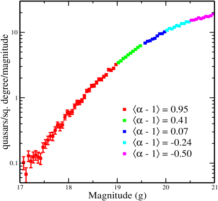
Figure 2.— Weighted number counts per magnitude per square degree in the 5 magnitude bins for quasars with photometric redshift between $1<z<2.2$.

4. Results

4.1. Lensing Origin of the Signal

In order to investigate the lensing origin of the signal, we first measured the quasar-galaxy correlations $w_{\rm GQ}(\theta,m)$ as a function of quasar magnitude in a given band. In Figure 2 we show the number counts of quasars as a function of magnitude in the $g$ band. We separated the $g$-selected quasar sample into five magnitude ranges and estimated the corresponding value of $\langle\alpha-1\rangle$ from power law fits in each bin. The results are presented in Table 1. As can be seen, the values of $\langle\alpha-1\rangle$ are greater than zero for the three brighter magnitude bins. Therefore, due to the magnification bias, we expect to find an excess of such quasars in the vicinity of foreground lenses. In a similar way, we expect a deficit of quasars with $g>20$.

Magnitude	$\langle\alpha-1\rangle$
$17~{}~{}<~{}g~{}<~{}19~{}~{}$	$~{}0.95$
$19~{}~{}<~{}g~{}<~{}19.5$	$~{}0.41$
$19.5<~{}g~{}<~{}20~{}~{}$	$~{}0.07$
$20~{}~{}<~{}g~{}<~{}20.5$	$-0.24$
$20.5<~{}g~{}<~{}21~{}~{}$	$-0.50$

Table 1The weighted mean value of $\alpha(m)-1=2.5\,\mathrm{dlogN_{0}}(m)/\mathrm{d}m-1$ obtained from power law fits in different magnitude bins in the $g$ band. The values obtained in all five bands are presented in Table 2.

The corresponding quasar-galaxy correlation functions in each magnitude bin are shown in Figure 3. As expected, the brightest quasar sample with the steepest number count slope showed the strongest positive cross-correlation, with the signal amplitude dropping and eventually changing to an anti-correlation as $\langle\alpha-1\rangle$ decreases. At large angles, we see a flat signal consistent with zero for all five quasar magnitude bins. This first test verified qualitatively that the measured signal satisfied the first of the two criteria described at the end of §2: amplitude variation as a function of quasar magnitude.

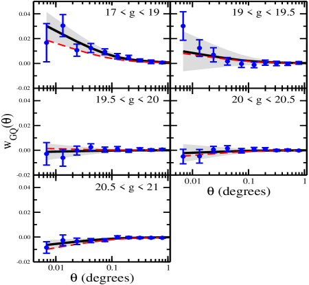
Figure 3.— Measurements of $w_{\rm GQ}(\theta)$ as a function of quasar $g$ band magnitude. Error bars are the $1\sigma$ errors based on the jack-knife covariance (Equation 12). The dark solid curve is the fitting model and the light dashed curve is the expected curve from the number counts $\langle\alpha-1\rangle$. The shaded region indicates the $1\sigma$ range on the fitted value of $\langle\alpha-1\rangle$. Fitted and expected values for each magnitude bin are given in Table 2. For angular scales larger than 1 degree, the measurements were consistent with zero in all five magnitude bins.

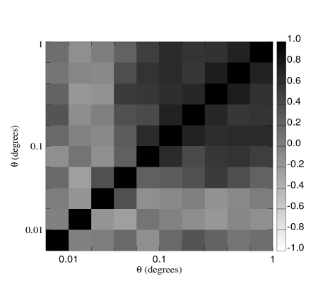
Figure 4.— Normalized covariance matrix for the $17<g<19$ measurement of $w_{\rm GQ}(\theta)$. For a given pair of angular bins ($i$ and $j$), the normalized covariance matrix is given by $C(\theta_{i},\theta_{j})/\sqrt{C(\theta_{i},\theta_{i})C(\theta_{j},\theta_{j})}$. The level of correlation between angular bins is roughly consistent for all of the measurements of $w_{\rm GQ}(\theta)$.

We can now quantify this agreement by using the model given in §2 and the covariance matrices measured using Equation 12 (see Figure 4) to fit the measured data points and estimate the value of $\langle\alpha-1\rangle$ in each magnitude bin. These fits are shown with the solid black line in Figure 3 and the one-sigma uncertainty by the shaded region. The value of the parameter $\langle\alpha-1\rangle$ obtained in this manner can be compared to the one directly measured from the quasar number counts. The expected measurement based on the quasar number counts is shown by the dashed red line. For all five $g$-selected magnitude bins, we find agreement between the fitted and measured values of $\langle\alpha-1\rangle$ as a function of quasar magnitude. This demonstrates that the behavior of the signal quantitatively follows both the amplitude and the angular variations expected from magnification bias.

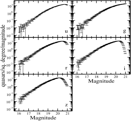
Figure 5.— Number counts per magnitude per square degree in the 5 filters for quasars with photometric redshift between $1<z<2.2$. The original sample is magnitude limited in the $g$ filter. The effective color cuts resulting from the quasar selection lead to incompleteness in the other filters at the faint end.

We repeated similar measurements using magnitude-limited samples in each of the other four SDSS bands. The quasar number counts in all five bands are given in Figure 5. As mentioned above, the quasars were magnitude limited in $g$. For the other bands, the combination of effective color cuts for the sample and intrinsic scatter led to strong incompleteness for magnitudes fainter than 20. For the purpose of separating the sample into magnitude bins, the turn-over point set the faintest limit for each band. The results for these measurements are summarized in Table 2. As with the $g$-selected measurements, cross-correlations in the other four filters found qualitative and quantitative agreement with the expected magnitude bias variation with $\langle\alpha-1\rangle$.

4.2. Optimal Stacking and Detection Significance

Having shown that the signal follows the theoretical expectations as a function of magnitude, we combined these measurements to quantify the significance of the global detection of cosmic magnification. Instead of separating the signal into five magnitude bins, we measured the signal integrated over all magnitudes weighted with different powers of $(\alpha(m)-1)^{n}$. In Figure 5, we show the number count relations in each of the five SDSS filters and Figure 6 plots the corresponding values of $(\alpha(m)-1)^{n}$ for $n=1$ and $2$. These plots are made by measuring $\langle\alpha-1\rangle$ in narrow magnitude bins over the full range and then interpolating over the bins with a cubic spline.

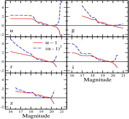
Figure 6.— $\alpha-1$ and $(\alpha-1)^{2}$ as a function of magnitude in the 5 filters for quasars with photometric redshift between $1<z<2.2$. For the $u$, $r$, $i$, and $z$ bands, incompleteness in the number counts at the faint end causes $\alpha-1$ to rapidly diverge, making a direct measurement of the expected anti-correlation in these filters very difficult.

$\bullet$ Mean correlation function: by simply averaging the signal from all quasars, i.e. considering the case $n=1$, we recover Equation 2, where $\langle\alpha-1\rangle$ is given by integration over the full magnitude range of the sample. The effects of bright and faint quasars generally canceled each other, resulting in the small values of $\langle\alpha-1\rangle$ found in Table 2. Figure 7 shows the results for all five SDSS filters, along with expected and fitted curves for $\langle\alpha-1\rangle$. As with the magnitude-selected samples, we see generally good agreement between the expected and observed signals. Note that all the data points are below the one-percent level.

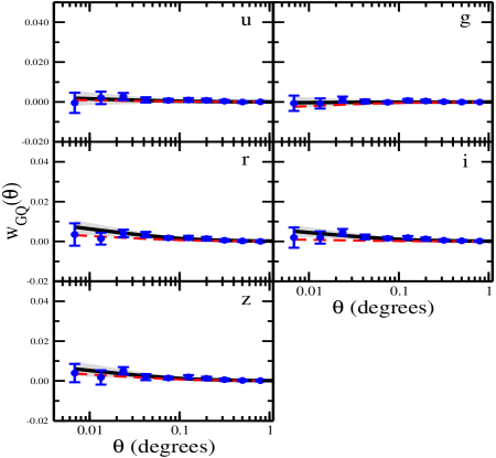
Figure 7.— Same as Figure 3, but over the full magnitude range in each wavelength band. The range on the y-axis is the same as in Figure 3 to provide an easier comparison of the relative amplitude for samples where we do and do not expect a strong lensing signal. Fitted and expected values for $\langle\alpha-1\rangle$ are given in Table 2. The correlation between angular bins for each measurement is consistent with that shown in Figure 4 to first order.

$\bullet$ Optimal correlation function: as shown by Ménard & Bartelmann (2002), using $n=2$ (i.e. looking at the second-order moment of the signal as a function of magnitude) optimally weights the expected lensing signal. This maximizes the S/N of the detection since the signal is weighted proportionally to the expectations. With the extra factor of $\alpha(m)-1$, the expected signal is:

$$w_{\rm GQ}^{\rm optimal}(\theta) = \langle(\alpha(m)-1)^{2}\rangle\times w_{0}(\theta)$$ (13)

$$= \frac{\int\mathrm{d}m\,N(m)\,(\alpha(m)-1)^{2}}{\int\mathrm{d}m\,N(m)}\times w_{0}(\theta)$$

$$= \langle\alpha-1\rangle_{E}\times w_{0}(\theta)\,.$$

The corresponding signal can be measured by weighting each quasar by a factor of $\alpha(m)-1$ and by calculating the cross-correlation in the manner described by Equations 10 and 11. Rather than largely counter-acting each other as seen in Figure 7, the positive and negative correlations from the bright and faint end of the quasar number counts now act in concert and benefit from the statistical power of the entire quasar population. The corresponding results are presented in Figure 8. Once again, we find a very good agreement between the model and the observations for all five bands.

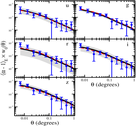
Figure 8.— Same as Figure 7, but for $w_{\rm GQ}^{\rm optimal}(\theta)$, which uses quadratic weighting to enhance the lensing S/N (Equation 13). Fitted and expected values for $\langle\alpha-1\rangle_{E}$ are given in Table 2. The correlation between angular bins for each measurement is consistent with that shown in Figure 4 to first order.

Using this optimally-weighted correlation function and the associated covariance matrix, we can assess the significance of our detection. By comparing the corresponding $\chi^{2}$ values of $w_{\rm GQ}^{\rm optimal}(\theta)$ against the null for 18 angular bins, we detect the signal at 4.1$\sigma$, 8.1$\sigma$, 4.8$\sigma$, 5.4$\sigma$ and 4.8$\sigma$ in the $u$, $g$, $r$, $i$ and $z$ bands respectively. If we consider only the angular scales $\leq 1^{\circ}$, as shown in Figure 8, the significance of the detection remains nearly the same.

Given the high S/N provided by the optimally-weighted estimator, we can compare the angular variation of the measured signal to theoretical expectations. As can be seen in Fig.8, we find consistency from $0.3^{\prime}$ to $1\deg$, i.e. over more than two orders of magnitude in scale. This allows us to validate the second criterion from §2: the match of the angular variation of the signal with the predicted cross-correlation function. Considering an effective redshift of $z=0.3$ for the foreground galaxy population, we find that the detected magnification signal probes scales ranging from $\sim 60h^{-1}$ kpc to $10$ Mpc.

Observing both the first and second moments of the lensing signal as a function of magnitude to give the expected behavior as a function of the observed values of $\alpha(m)-1$ is an excellent indication that we are observing the signal originating from gravitational lensing.

4.3. Systematics

As seen in §1, accurate measurements of galaxy and quasar number counts can suffer from a number of biases: seeing variations, stellar contamination, dust extinction, redshift overlap, etc. To verify that our measurements are not affected by these effects, we have performed a number of checks.

To test for stellar contamination in our sample of quasars, we cross-correlated stars in the $17<r<21$ range with the $g$ band selected quasars, $w_{\rm SQ}(\theta)$, both with and without optimal weighting. Unlike galaxies or quasars, the local stellar density is not well approximated by the global mean density. As a result, we do not expect (and do not observe) a null correlation between stars and quasars (or stars and galaxies). Rather, our observed $w_{\rm SQ}(\theta)$ was consistent with the observed galaxy-star cross-correlation, both of which are consistent with a very small ($\sim$ 1%) level of stellar contamination. More importantly, when we optimally weighted $w_{\rm SQ}(\theta)$, the signal was consistent with zero at all angular scales, as would be expected for a stellar density independent of $\alpha(m)-1$. This was in marked contrast to $w_{\rm GQ}^{\rm optimal}(\theta)$, detected at $8\sigma$. Cross-correlations with local seeing produced similar results.

We also tested the robustness of the photometric redshift likelihood by applying a series of redshift likelihood thresholds (i.e. requiring that the probability that the quasar was within the upper and lower redshift ranges specified by the quasar photometric redshift algorithm was above a given value: 50%, 60%, 70%, etc.). In all cases, the resulting galaxy-quasar cross-correlation was consistent with measurements made with no threshold, verifying that our signal was not dominated by low probability outliers. Finally, a cross-correlation with low redshift quasars produced a large amplitude, positive signal. However, this last point was sensitive to a restrictive cut on the quasar redshift probability ($>80\%$) due to a strong shift in the probability distributions for quasars below $z\sim 1$; higher redshift quasars tended to have much higher redshift probabilities ($\sim 0.8$) than low redshift quasars (peaks around 0.5 and 0.8).

Next, we checked for possible contamination by large, bright galaxies. As described in Mandelbaum et al. (2005), the estimation of the density of faint sources around bright extended objects can be biased induced by uncertainties in the sky subtraction. We do not expect the sky subtraction issues to be as significant since our quasars are point sources, but, as described in §3, we applied a 60^′′ mask around all $r<16$ galaxies. Measurements with and without these masks were identical, but we included the masks in our final analysis to avoid any unforeseen effects.

Finally, a bias that is not related to the data analysis but that might be intrinsically present is extinction by dust. Indeed, the presence of dust around galaxies is expected to redden and extinct background sources. So far, the amount of dust on large scales has been poorly constrained and its effects on measurements of quasar-galaxy correlations has been uncertain. However, our analysis indicates that the deficit of quasars due to dust extinction is subdominant to the density changes induced by gravitational lensing. Indeed, the fact that the measured signal for the first and second moments behaves as expected as a function of the slope number counts, $\alpha(m)-1$, indicates that the signal might not be contaminated by other sources than gravitational lensing. Biases like dust extinction or the above-mentioned effects are not expected to scale proportionally to $\alpha(m)-1$ and would therefore affect the first and second moments of the signal in different ways. This would prevent the simultaneous agreements found above. Therefore we conclude that our current measurements are not significantly affected by biases, but a parallel effort is underway to quantify the reddening effects of the lensing galaxies more precisely.

5. Discussion & Future Applications

In this paper we have presented a detection of cosmic magnification obtained by cross-correlating distant quasars and foreground galaxies. Using data from approximately 3800 square degrees of the SDSS photometric sample, we have cross-correlated the position of $\sim 200,000$ photometrically selected quasars and large-scale structures traced by over 13 million galaxies, and we have detected a signal on angular scales from 20^′′ to 1 degree at high significance.

The magnification bias due to weak lensing gives rise to an excess or a deficit of background sources in the vicinity of foreground galaxies depending on the value of the power-law slope of the source number counts: $\mathrm{\alpha}(m)=2.5\,\mathrm{dlog\,N_{0}}(m)/\mathrm{d}m$. Our measurements of the galaxy-quasar cross-correlation function exhibit the expected behavior: bright quasars, with steep number counts, appear to be in excess around galaxies and large-scale structures, and faint quasars with shallow number counts are seen to be in deficit. On all scales, we find $w_{\rm GQ}(m)\propto(\alpha(m)-1)$ in the five SDSS bands, as expected.

We have measured the first and second moments of the signal as a function of quasar magnitude and the results are in very good agreement with what is expected from the magnification bias: depending on the band, the first moment gives an amplitude consistent with zero or smaller than $\sim 5\times 10^{-3}$, as a result of the opposite effects arising from the bright and the faint quasars. The second moment, which turns out to be the optimal signal estimator, exhibits a strong signal detected at $>4\sigma$ in all five SDSS filters and reaching up to 8.1$\sigma$ in the $g$-band. The quasars are magnitude selected in the $g$-band, giving us the largest sample in this band (other bands lose quasars at the faint end due to the effective color cuts in these bands), so the difference in the signal-to-noise in the other bands relative to $g$ is unsurprising. Using this estimator we find the angular dependence of the signal to be in very good agreement with theoretical estimations of lensing by large-scale structures. Our measurements probe physical scales ranging from $60\,h^{-1}\,$kpc to $10\,h^{-1}\,$Mpc at the mean lens redshift. Since we do not expect the biases from systematic errors to scale proportionally to $\alpha(m)-1$, the simultaneous agreement of the first and second moments of the signal as a function of magnitude indicates that these systematic biases (including dust extinction) do not significantly affect our measurements.

The SDSS quasar and galaxy samples used in our analysis are significantly larger, more uniform and better characterised than any data sets used for this measurement previously. We have shown that biases including seeing variations, stellar contamination, sky subtraction issues and errors in the photometric redshifts are well controled and do not significantly affect the measurements. Whereas previously claimed detections reported a signal much larger than theoretical predictions, our measurement shows, for the first time, the expected amplitude and angular dependence for the standard cosmological model and a realistic galaxy biasing. As such, we conclude that the disagreement between theoretical predictions and previous measurements was most likely due to larger systematic effects in these data sets which could not be adequately controled.

The successful detection of cosmic magnification opens the door to a number of applications: as mentioned in §2, cosmic magnification is a function of the first moment of the galaxy halo occupation distribution (HOD) on all angular scales. Conversely, the galaxy auto-correlation function, $w(\theta)$, is a strong function of the second moment of the HOD. Thus, measuring these two quantities for the same sample of galaxies will provide us with constrains on both moments, and therefore probe the scales on which the galaxy biasing becomes stochastic. Such an analysis can then be carried out as a function of galaxy type, redshift, etc. and provide interesting constraints on our understanding of galaxies and large-scale structures.

As noted in §1, our measurements of cosmic magnification constrain the projected galaxy-mass correlation in much the same way as galaxy-galaxy lensing, although that method is based on galaxy shapes and measurements of shear. This complementarity is a particularly useful cross-check since the dominant sources of systematic error for the two methods are different (PSF anisotropy for the galaxy-galaxy shear measurements vs. photometric calibration for the magnification bias). Furthermore, using quasars as sources, cosmic magnification allows for probing lensing at higher redshifts: the sources used for SDSS galaxy-galaxy lensing studies are used as lenses for measurements of quasar-galaxy correlations. Finally, as is the case for cosmic shear, higher-order statistics can also be investigated in the context of lensing-induced quasar-galaxy correlations (Ménard et al. 2003). We also note that the techniques used for efficient quasar selection are readily applicable to next generation of large, multi-band surveys. Cosmic magnification is therefore an excellent complement to planned cosmic shear surveys.

In a future work we will use measurements of quasar-galaxy correlations to generate the first constraints on the galaxy HOD and cosmological parameters obtained from cosmic magnification. Likewise, projects are underway to use cosmic magnification to measure the extent of galaxy dust halos as well dark matter halo ellipticities.

Table 2Quasar counts, $\langle\alpha-1\rangle$ from the number count slopes in each magnitude bin, $\langle\alpha-1\rangle$ from fitting observed $w_{\rm GQ}(\theta)$ to the weak-lensing model given in Equation 6 and detection significance for the optimal estimator in each filter. For the optimal estimator, the full magnitude range is used and the values of $\langle\alpha-1\rangle$ are for $\langle\alpha-1\rangle_{E}$ as given in Equation 13. Detection significance is given in multiples of standard deviation ($\sigma$).

Magnitude Limit	Quasar Counts	$\langle\alpha-1\rangle$	Fitted $\langle\alpha-1\rangle$	$\sigma$
$17<u<19$	6774	$+0.97$	$+1.63\pm 0.70$
$19<u<19.5$	9001	$+0.42$	$+0.19\pm 0.95$
$19.5<u<20$	16648	$+0.07$	$-0.27\pm 0.39$
$20<u<20.3$	14824	$-0.11$	$+0.04\pm 0.55$
$20.3<u<20.6$	18524	$-0.37$	$-0.08\pm 0.34$
$17<u<20.6$	65610	$+0.05$	$+0.09\pm 0.19$
Optimal	65610	$+0.18$	$+0.19\pm 0.09$	4.1
$17<g<19$	8054	$+0.95$	$+1.53\pm 0.57$
$19<g<19.5$	10312	$+0.41$	$+0.49\pm 0.81$
$19.5<g<20$	18148	$+0.07$	$-0.06\pm 0.33$
$20<g<20.5$	28751	$-0.24$	$-0.12\pm 0.36$
$20.5<g<21$	39567	$-0.50$	$-0.32\pm 0.19$
$17<g<21$	104683	$-0.12$	$-0.02\pm 0.14$
Optimal	104683	$+0.22$	$+0.20\pm 0.05$	8.1
$16<r<18.5$	4212	$+1.19$	$+1.84\pm 0.79$
$18.5<r<19$	6120	$+0.65$	$+1.36\pm 0.86$
$19<r<19.5$	12101	$+0.35$	$-0.30\pm 0.60$
$19.5<r<20$	21141	$+0.03$	$+0.14\pm 0.25$
$20<r<20.3$	18137	$-0.25$	$-0.11\pm 0.34$
$16<r<20.3$	61596	$+0.16$	$+0.37\pm 0.17$
Optimal	61596	$+0.20$	$+0.18\pm 0.12$	4.8
$16<i<18.5$	5609	$+1.08$	$+1.66\pm 0.81$
$18.5<i<19$	7813	$+0.56$	$+1.06\pm 0.96$
$19<i<19.5$	15236	$+0.23$	$-0.10\pm 0.76$
$19.5<i<20$	26173	$-0.06$	$+0.21\pm 0.33$
$20<i<20.2$	17687	$-0.51$	$-0.11\pm 0.57$
$16<i<20.2$	72391	$+0.05$	$+0.26\pm 0.14$
Optimal	72391	$+0.21$	$+0.24\pm 0.13$	5.3
$16<z<18.5$	5812	$+1.00$	$+1.58\pm 0.77$
$18.5<z<19$	8047	$+0.62$	$+0.97\pm 0.85$
$19<z<19.5$	16056	$+0.29$	$-0.05\pm 0.37$
$19.5<z<19.8$	15240	$+0.13$	$-0.02\pm 0.39$
$19.8<z<20.1$	20177	$-0.27$	$-0.25\pm 0.49$
$16<z<20.1$	65207	$+0.19$	$+0.31\pm 0.18$
Optimal	65207	$+0.21$	$+0.25\pm 0.11$	4.8

References

- (1)
- Abazajian et al. (2005) Abazajian, K., et al. 2005, AJ, in press
- Bacon et al. (2000) Bacon, D.J., Refregier, A.R., Ellis, R.S, 2000, MNRAS, 318, 625
- Bartelmann & Schneider (1994) Bartelmann, M. & Schneider, P., 1994, A&A, 284, 1
- Bartelmann (1995) Bartelmann, M. 1995, A&A, 298, 661
- Bartelmann & Schneider (1993b) Bartelmann, M. & Schneider, P., 1993b, A&A, 271, 421
- Bartelmann et al. (1994) Bartelmann, M., Schneider, P., & Hasinger, G., 1994, A&A, 290, 399
- Bartsch et al. (1997) Bartsch, A., Schneider, P., & Bartelmann, M., 1997, A&A, 319, 375
- Benítez & Martínez-González (1995) Benítez, N., & Martínez-González, 1995, ApJLett, 339, 53
- Blanton et al. (2003) Blanton, M.R., Lupton, R.H., Maley, F.M., Young, N., Zehavi, I., and Loveday, J. 2003, AJ, 125, 2276
- Boyle et al. (1988) Boyle, B.J., Fong, R. & Shanks, T., 1988, MNRAS, 231, 897
- Brown et al. (2003) Brown, M.L., Taylor, A.N., Bacon, D.J., Gray, M.E., Dye, S., & Meisenheimer, K. 2003, MNRAS, 341, 100
- Brainerd, Blandford & Smail (1996) Brainerd, T. G., Blandford, R. D., & Smail, I. 1996, ApJ, 466, 623
- Cooray (1999) Cooray, A. R. 1999, A&A, 348, 673
- Croom & Shanks (1999) Croom, S. M. & Shanks, T. 1999, MNRAS, 307, L17
- dell’Antonio & Tyson (1996) dell’Antonio, I. P. & Tyson, J. A. 1996, ApJ, 473, L17
- Dolag & Bartelmann (1997) Dolag, K. & Bartelmann, M. 1997, MNRAS, 291, 446
- Ferreras et al. (1997) Ferreras, I. , Benitez, N. & Marti nez-Gonzalez, E. 1997, AJ, 114, 1728
- Fischer et al. (2000) Fischer, P. et al. 2000, AJ, 120, 1198
- Fugmann (1990) Fugmann, W., 1990, A&A, 240, 11
- Fukugita et al. (1996) Fukugita, M., Ichikawa, T., Gunn, J.E., Doi, M., Shimasaku, K., and Schneider, D.P. 1996, AJ, 111, 1748
- Gaztañaga (2003) Gaztañaga, E. 2003, ApJ, 589, 82
- Griffiths et al. (1996) Griffiths, R.E., Casertano, S., Im, M., & Ratnatunga, K.U. 1996, MNRAS, 282, 1159
- Guimarães et al. (2001) Guimarães, A. C. C., van De Bruck, C., & Brandenberger, R. H. 2001, MNRAS, 325, 278
- Gunn et al. (1998) Gunn, J.E., et al. 1998, AJ, 116, 3040
- Hoekstra et al. (2002a) Hoekstra et al., 2002, ApJ, 572, 55
- Hoekstra et al. (2002b) Hoekstra, H., et al, 2002, ApJ, 577, 604
- Hoekstra et al. (2003) Hoekstra, H. et al. 2003, astroph/0306515
- Hoekstra (2003) Hoekstra, H. 2003, IAU Symposium, 216,
- Hogg et al. (2001) Hogg, D.W., Finkbeiner, D.P., Schlegel, D.J., and Gunn, J.E. 2001, AJ, 122, 2129
- Hudson et al. (1998) Hudson, M. J., Gwyn, S. D. J., Dahle, H., & Kaiser, N. 1998, ApJ, 503, 531
- Ivezic et al. (2004) Ivezic, Z., et al. 2004, AN, 325, 583
- Jain, Scranton & Sheth (2003) Jain, B., Scranton, R. & Sheth, R.K., 2003, MNRAS, 345, 62
- Jarvis et al. (2003) Jarvis et al., 2003, AJ, 125, 1014
- Kravtsov et al. (2004) Kravtsov et al., 2004, ApJ, 609, 35
- Landy & Szalay (1993) Landy, S. D., & Szalay, A. S. 1993, ApJ, 412, 64
- Lin et al. (1999) Lin, H., Yee, H. K. C., Carlberg, R. G., Morris, S. L., Sawicki, M., Patton, D. R., Wirth, G., & Shepherd, C. W. 1999, ApJ, 518, 533
- Lupton, Gunn & Szalay (1999) Lupton, R.H., Gunn, J.E., and Szalay, A.S. 1999, AJ, 118, 1406
- Maddox et al. (1990) Maddox, S. J., Efstathiou, G., Sutherland, W. J., & Loveday, J. 1990, MNRAS, 243, 692
- Mandelbaum et al. (2005) Mandelbaum, R. et al. 2005, astro-ph/0501201
- Massey et al. (2004) Massey et al. 2004, astro-ph/0404195.
- McKay et al. (2001) McKay, T. A. et al. 2002, astro-ph/0108013
- Ménard & Bartelmann (2002) Ménard, B. & Bartelmann, M., 2002, A&A, 386, 784
- Ménard et al. (2003) Ménard, B., Hamana, T., Bartelmann, M., & Yoshida, N. 2003, A&A, 403, 817
- Ménard et al. (2003) Ménard, B., Bartelmann, M., & Mellier, Y. 2003, A&A, 409, 411
- Myers et al. (2003) Myers, A. D., Outram, P. J., Shanks, T., Boyle, B. J., Croom, S. M., Loaring, N. S., Miller, L., & Smith, R. J. 2003, MNRAS, 342, 467
- Myers et al. (2005) Myers A.D., Outram P.J., Shanks T., Boyle B.J., Croom S.M., Loaring N.S., Miller L. & Smith R.J., astro-ph/0502481
- Narayan (1989) Narayan, R. 1989, ApJ, 339, L53
- Navarro, Frenk, & White (1997) Navarro, J. F., Frenk, C. S., & White, S. D. M. 1997, ApJ, 490, 493
- Norman & Impey (1999) Norman, D. J. & Impey, C. D. 1999, AJ, 118, 613
- Norman & Williams (2000) Norman, D.J. & Williams, L.L.R. 2000, ApJ, 119, 2060
- Pier et al. (2003) Pier, J.R., Munn, J.A., Hindsley, R.B., Hennessy, G.S., Kent, S.M., Lupton, R.H., and Ivezic, Z. 2003, AJ, 125, 1559
- Refregier (2003) Refregier, A. 2003, ARA&A, 41, 645
- Rhodes et al. (2001) Rhodes, J., Refregier, A., Groth, E.J., 2001, ApJ, 552, L85
- Richards et al. (2002) Richards, G.T., et al 2002, AJ, 123, 2945
- Richards et al. (2004) Richards, G.T. et al 2004, ApJS, 155, 257
- Rodrigues-Williams & Hogan (1994) Rodrigues-Williams, L. L. & Hogan, C. J. 1994, AJ, 107, 451
- Rodrigues-Williams & Hawkins (1995) Rodrigues-Williams, L. L. & Hawkins, M. R. S., 1995, in Dark Matter, AIP conference proceedings 336, College Park, MD, 1994, p. 331
- Sanz et al. (1997) Sanz, J. L., Marti nez-González, E. & Benitez, N. 1997, MNRAS, 291, 418
- Schneider et al. (1992) Schneider, P., Ehlers, J., & Falco, E.E. 1992, Gravitational Lenses(Heidelberg:Springer)
- Scranton et al. (2002) Scranton, R. et al. 2002, ApJ, 579, 48
- Seldner & Peebles (1979) Seldner, M., & Peebles, P. J. E. 1979, ApJ, 227, 30
- Seitz & Schneider (1995) Seitz, S. & Schneider, P., 1995b, A&A, 302, 9
- Seljak et al. (2004) Seljak, U. et al., 2004, astro-ph/0406594
- Sheldon et al. (2004) Sheldon, E. et al., 2004, AJ, 127, 2544
- Smith et al. (2001) Smith, D. R., Bernstein, G. M., Fischer, P., & Jarvis, M. 2001, ApJ, 551, 643
- Smith et al. (2002) Smith, J.A., et al 2002, AJ, 123, 2121
- Spergel et al. (2003) Spergel, D. et al, 2003, astro-ph/0302209
- Stoughton et al. (2002) Stoughton, C., et al 2002, AJ, 123, 485
- Takada & Hamana (2003) Takada, M., & Hamana, T. 2003, MNRAS, 346, 949
- Van Waerbeke et al. (2000) Van Waerbeke, L. et al., 2000, A&A, 358, 30
- Van Waerbeke et al. (2002) Van Waerbeke et al., 2002, A&A, 393, 369
- Van Waerbeke & Mellier (2003) Van Waerbeke & Mellier, 2003, astro-ph/0305089
- Williams & Irwin (1998) Williams, L. L. R. & Irwin, M. 1998, MNRAS, 298, 378
- Wilson et al. (2001) Wilson, G., Kaiser, N., Luppino, G. A., & Cowie, L. L. 2001, ApJ, 555, 572
- Weinstein et al. (2004) Weinstein, M.A. et al. 2004, ApJS, 155, 243
- Wu & Han (1995) Wu, X.-P. & Han, J., 1995, MNRAS, 272, 705
- York et al. (2000) York, D.G. et al., 2000, AJ., 120, 1579.
- Zehavi et al. (2004) Zehavi, I. et al., 2004, astro-ph/0408569