Deviation of light curves of gamma-ray burst pulses from standard forms due to the curvature effect of spherical fireballs or uniform jets

Abstract

As revealed previously, under the assumption that some pulses of gamma-ray bursts are produced by shocks in spherical fireballs or uniform jets of large opening angles, there exists a standard decay form of the profile of pulses arising from very narrow or suddenly dimming local (or intrinsic) pulses due to the relativistic curvature effect (the Doppler effect over the spherical shell surface). Profiles of pulses arising from other local pulses were previously found to possess a reverse S-feature deviation from the standard decay form. We show in this paper that, in addition to the standard decay form shown in Qin et al. (2004), there exists a marginal decay curve associated with a local $\delta$ function pulse with a mono-color radiation. We employ the sample of Kocevski et al. (2003) to check this prediction and find that the phenomenon of the reverse S-feature is common, when compared with both the standard decay form and the marginal decay curve. We accordingly propose to take the marginal decay curve (whose function is simple) as a criteria to check if an observed pulse could be taken as a candidate suffered from the curvature effect. We introduce two quantities $A_{1}$ and $A_{2}$ to describe the mentioned deviations within and beyond the $FWHM$ position of the decay phase, respectively. The values of $A_{1}$ and $A_{2}$ of pulses of the sample are calculated, and the result suggests that for most of these pulses their corresponding local pulses might contain a long decay time relative to the time scale of the curvature effect.

1 Introduction

In spite of the temporal structure of gamma-ray bursts (GRBs) varying drastically, it is generally believed that some well-separated pulses represent the fundamental constituent of GRB time profiles (light curves) and appear as asymmetric pulses with a fast rise and an exponential decay (FRED)(see, e.g., Fishman et al. 1994).

Due to the large energies and the short timescales involved, the observed gamma-ray pulses are believed to be produced in a relativistically expanding and collimated fireball. The observed FRED structure was interpreted by the curvature effect as the observed plasma moves relativistically towards us and appears to be locally isotropic (e.g., Fenimore et al. 1996, Ryde & Petrosian 2002; Kocevski et al. 2003, hereafter Paper I). Several investigations on modeling pulse profiles have previously been made (e.g., Norris et al. 1996; Lee et al. 2000a, 2000b; Ryde et al. 2000, 2002). Several flexible functions describing the profiles of individual pulses based on empirical relations were presented. As derived in details in Ryde et al. (2002), a FRED pulse can be well described by equation (22) or (28) there. Using this equation, they could characterize individual pulse shapes created purely by relativistic curvature effects in the context of the fireball model.

Qin (2002) derived in details the flux intensity based on the model of highly symmetric expanding fireballs, where the Doppler effect of the expanding fireball surface is the key factor to be concerned. The formula is applicable to cases of relativistic, sub-relativistic, and non-relativistic motions as no terms are omitted in the corresponding derivation. With this formula, Qin (2003) studied how emission and absorbtion lines are affect by the effect. Recently, Qin et al. (2004, hereafter Paper II) rewrote this formula in terms of the integral of the local emission time, which is in some extent similar to that presented in Ryde & Petrosian (2002), where relation between the observed light curve and the local emission intensity is clearly illustrated. Based on this model, many characteristics of profiles of observed gamma-ray burst pulses could be explained. Profiles of FRED pulse light curves are mainly caused by the fireball radiating surface, where emissions are affected by different Doppler factors and boostings due to different angles to the line of sight, and they depend also on the width and structure of local pulses as well as rest frame radiation mechanisms. This allows us to explore how other factors such as the width of local pulses affect the profile of the light curve observed.

Revealed in Paper II, there exists only a slowly decaying phase in the light curve associated with a local $\delta$ function pulse, for which no rising phase can be seen. For a local pulse with a certain width, the light curve observed would contain both the rising and decaying parts. It was revealed that light curves arising from very narrow local pulses and those arising from suddenly dimming local pulses share the same form of profiles in their decaying phase, which was called a standard decay form (see Paper II). For a common local pulse for which the decaying time is not short enough, the profile of the decay portion of the resulting light curve would significantly deviate from the standard form. It is interesting that, the deviation could be characterized by the feature of a reverse “S” (see Paper II Fig. 5). We wonder if this indeed holds for FRED pulse GRBs. If it holds, how can we describe this deviation? Motivated by this, we explore quantitatively in this paper the deviation of light curves of gamma-ray burst pulses from the so-called standard decay form. A sample of FRED pulse sources will be studied.

The paper is organized as follows. In section 2, we analyse the deviation of light curve pulses associated with gamma-ray burst spherical fireballs or uniform jets, from the standard form and a marginal curve. In section 3, we examine the deviation deduced from a sample detected by the BATSE instrument on board the Compton Gamma Ray Observatory. Discussion and conclusions are presented in the last section.

2 Theoretical analysis

As derived in details in Qin (2002) and Paper II, the expected count rate of a fireball within frequency interval $[\nu_{1},\nu_{2}]$ can be calculated by

$$C(\tau)=\frac{2\pi R_{c}^{3}\int_{\widetilde{\tau}_{\theta,\min}}^{\widetilde{\tau}_{\theta,\max}}\widetilde{I}(\tau_{\theta})(1+\beta\tau_{\theta})^{2}(1-\tau+\tau_{\theta})d\tau_{\theta}\int_{\nu_{1}}^{\nu_{2}}\frac{g_{0,\nu}(\nu_{0,\theta})}{\nu}d\nu}{hcD^{2}\Gamma^{3}(1-\beta)^{2}(1+\frac{\beta}{1-\beta}\tau)^{2}},$$ (1)

which is just equation (21) in Paper II. This formula was derived under the assumption that the fireball expands isotropically with a constant Lorentz factor $\Gamma>1$ and the radiation is independent of direction. Present in the formula, $\tau_{\theta}$ is a dimensionless relative local time defined by $\tau_{\theta}\equiv c(t_{\theta}-t_{c})/R_{c}$, where $t_{\theta}$ is the emission time (in the observer frame), called local time, of photons emitted from the concerned differential surface $ds_{\theta}$ of the fireball ($\theta$ is the angle to the line of sight), $t_{c}$ is a constant which could be assigned to any values of $t_{\theta}$, and $R_{c}$ is the radius of the fireball measured at $t_{\theta}=t_{c}$. In equation (1), $\widetilde{I}(\tau_{\theta})$ represents the development of the intensity magnitude in the observer frame, and $g_{0,\nu}(\nu_{0,\theta})$ describes the rest frame radiation mechanism, with $\nu_{0,\theta}$ being the rest frame emission frequency which is related to the observation frequency $\nu$ by the Doppler effect. Variable $\tau$ used in the formula is a dimensionless relative time defined by $\tau\equiv[c(t-t_{c})-D+R_{c}]/R_{c}$, where $D$ is the distance of the fireball to the observer, and $t$ is the observation time. As analyzed in Qin (2002) and Paper II, the relative time $\tau$ is confined by $1-\cos\theta_{\min}+(1-\beta\cos\theta_{\min})\tau_{\theta,\min}\leq\tau\leq 1-\cos\theta_{\max}+(1-\beta\cos\theta_{\max})\tau_{\theta,\max}$, and the integral limits $\widetilde{\tau}_{\theta,\min}$ and $\widetilde{\tau}_{\theta,\max}$ are determined by $\widetilde{\tau}_{\theta,\min}=\max\{\tau_{\theta,\min},(\tau-1+\cos\theta_{\max})/(1-\beta\cos\theta_{\max})\}$ and $\widetilde{\tau}_{\theta,\max}=\min\{\tau_{\theta,\max},(\tau-1+\cos\theta_{\min})/(1-\beta\cos\theta_{\min})\},$ respectively, where we assign $\theta_{\min}\leq\theta\leq\theta_{\max}$ and $\tau_{\theta,\min}\leq\tau_{\theta}\leq\tau_{\theta,\max}$.

A local $\delta$ function pulse, $\widetilde{I}(\tau_{\theta})=cI_{0}\delta(\tau_{\theta}-\tau_{\theta,0})/R_{c}$ (where $I_{0}$ and $\tau_{\theta,0}$ are constants), when inserting it into (1), would produce an observed light curve of equation (35) in Paper II, which is

$$C(\tau)=\frac{2\pi R_{c}^{2}I_{0}\int_{\nu_{1}}^{\nu_{2}}\frac{g_{0,\nu}(\nu_{0,\theta})}{\nu}d\nu}{hD^{2}}C_{0}(\tau),$$ (2)

with

$$C_{0}(\tau)\equiv\frac{(1+\beta\tau_{\theta,0})^{2}(1+\tau_{\theta,0}-\tau)}{\Gamma^{3}(1-\beta)^{2}(1+\frac{\beta}{1-\beta}\tau)^{2}}.$$ (3)

Note that the range of $\tau$, within which the radiation of the local $\delta$ function pulse over the concerned area is observable, is $1-\cos\theta_{\min}+(1-\beta\cos\theta_{\min})\tau_{\theta,0}<\tau<1-\cos\theta_{\max}+(1-\beta\cos\theta_{\max})\tau_{\theta,0}$ (see Paper II). As a product of the local $\delta$ function pulse, light curves $C(\tau)$ and $C_{0}(\tau)$ reflect nothing but the pure curvature effect. For $\Gamma\gg 1$, the term $\beta\tau/(1-\beta)$ in equation (3) could be written as $\beta\tau/(1-\beta)\simeq(t-t_{0})/(R_{c}/2\Gamma^{2}c)$, where $t_{0}$ is a constant. We find that $R_{c}/2\Gamma^{2}c$ is exactly the time scale of the curvature effect (see equation [5] in Paper I). (One can check that, in terms of local time, this curvature effect time scale becomes $R_{c}/c$.)

In the case of the local $\delta$ function pulse, as shown in Paper II equation (37), $\nu_{0,\theta}$ and $\nu$ are related by $\nu_{0,\theta}=[1+\beta\tau/(1-\beta)](1-\beta)\Gamma\nu/(1+\beta\tau_{\theta,0})$, from which one gets $d\nu_{0,\theta}/\nu_{0,\theta}=d\nu/\nu$. Thus, when taking $g_{0,\nu}(\nu_{0,\theta})$ as a $\delta$ function (i.e., when considering a mono-color radiation) and when interval $[\nu_{1},\nu_{2}]$ is large enough, $C(\tau)$ would become $C_{0}(\tau)$ (differing only by a factor). Thus, $C_{0}(\tau)$ represents the light curve arising from a local $\delta$ function pulse and associated with a mono-color radiation. As the radiation concerned (the GRB spectrum) is not a mono-color one and must last an interval of time, we call function $C_{0}(\tau)$ as a marginal decay curve.

As mentioned above, a sudden dimming or a very narrow local pulse could produce a standard decay form of light curves (see Paper II). According to Fig. 5 of Paper II, the standard form could be represented by equation (2). (Note that, a local $\delta$ function pulse is an extremely narrow local pulse, and it belongs to the class of suddenly dimming local pulses.) Shown in Preece et al. (1998, 2000), $\alpha_{0}=-1$ and $\beta_{0}=-2.25$ are typical values of the lower and higher indexes of the Band function spectrum, deduced from most GRBs observed. We thus define $C(\tau)$ associated with the rest frame Band function spectrum of $\alpha_{0}=-1$ and $\beta_{0}=-2.25$ as a standard decay form which was mentioned in Paper II previously.

With these two curves, we are able to explore how light curves associated with different local pulse forms deviate from standard ones, and with the deviation we might be able to estimate some parameters of local pulses.

Taking $\tau_{\theta,0}$=0, $\theta_{min}$=0, and $\theta_{max}=\pi/2$, we get $0<\tau<1$, and equation (3) becomes

$$C_{0}(\tau)=\frac{(1-\tau)}{\Gamma^{3}(1-\beta)^{2}(1+\frac{\beta}{1-\beta}\tau)^{2}}.$$ (4)

For the sake of comparison, we normalize light curves of (2) and (4) in intensity and re-scale its variable, $\tau$, by $\tau=a\tau^{\prime}+b$, so that the peak count rate is located at $\tau^{\prime}=0$ and the FWHM position of the decay portion is located at $\tau^{\prime}=0.2$ (see Paper II).

Formula (1) suggests that, except the state of the fireball ( i.e., $\Gamma$, $R_{c}$ and D), light curves of sources depend only on $\widetilde{I}(\tau_{\theta})$ and $g_{0,\nu}(\nu_{0,\theta})$. We assume in this paper the common empirical radiation form of GRBs as the rest frame radiation form, the so-called Band function (Band et al. 1993) that could well describe spectra of most sources (see, e.g., Schaefer et al. 1994; Ford et al. 1995; Preece et al. 1998, 2000), and adopt different forms of local pulses, $\widetilde{I}(\tau_{\theta})$ in equation (1), which will produce different light curves, to study the deviation from the standard forms.

Let us consider two local pulses. The first is a local pulse with an exponential rise

$$\widetilde{I}(\tau_{\theta})=I_{0}\exp(\frac{\tau_{\theta}-\tau_{\theta,\max}}{\sigma})\qquad\qquad\qquad(\tau_{\theta,\min}\leq\tau_{\theta}\leq\tau_{\theta,\max}),$$ (5)

and the second is a local pulse with an exponential decay

$$\widetilde{I}(\tau_{\theta})=I_{0}\exp(-\frac{\tau_{\theta}-\tau_{\theta,\min}}{\sigma})\qquad\qquad\qquad\qquad\qquad(\tau_{\theta,\min}\leq\tau_{\theta}).$$ (6)

Following Paper II, we take $\tau_{\theta,max}=10\sigma+\tau_{\theta,min}$ (in this case the interval between $\tau_{\theta,max}$ and $\tau_{\theta,\min}$ would be large enough to make the rising part of the local pulse close to that of the exponential pulse) and $\tau_{\theta,min}=0$. Light curves arising from these local pulses are normalized and re-scaled in the way mentioned above, which are shown in Fig. 1.

Figure 1: –Plots of the normalized and re-scaled light curve $C(\tau^{\prime})$ arising from the local exponential rise pulse (5) (the left panel), the local exponential decay pulse (6) (the middle panel), and three other local pulses (7) (dash line), (8) (dot line), and (9) (dash dot line) (the right panel). The solid and short dash lines represent the standard decay form and the marginal decay curve in the left and middle panels, respectively. A Band function rest frame radiation form with $\alpha_{0}=-1$ and $\beta_{0}=-2.25$, and the frequency range of 100 $\leq$ $\nu/\nu_{0,p}$$\leq$ 300, are adopted, and we take $\Gamma=100$, $\sigma$=0.02 (dash line), 0.2 (dot line), 2 (dash dot line), and 20 (dash dot dot line), respectively.

We find from Fig. 1 that there is no significant deviation of the light curves arising from local exponential rise pulses from the standard decay form in the decay portion of the light curve, just as what illustrated in Paper II. However, there are a significant “positive” deviation (over the standard form) of the light curves associated with local exponential decay pulses from the standard decay form within the range of $\tau^{\prime}\in[0.0,0.2]$, and a significant “negative” deviation in the range of $\tau^{\prime}>0.2$, which we call a reverse “S” deviation characteristic. In addition, one finds from Fig. 1 that there exists a “negative” deviation of the standard decay form from the marginal decay curve within the range of $\tau^{\prime}>0.2$, but within the range of $\tau^{\prime}\in[0.0,0.2]$ there is no deviation between the two.

We define the positive and negative deviation areas from the standard decay form (and/or the marginal decay curve) as $A_{1}$ and $A_{2}$, respectively. Relation between $A_{1}$ and $A_{2}$ and those between these areas and $\sigma$ are presented in Fig. 2 (here $A_{2}$ is calculated within the range of $\tau^{\prime}\in[0.2,2.0]$, as light curves of local exponential decay pulses overlap each other in the range of $\tau^{\prime}>2$). As shown in Fig. 2, $logA_{1}$ is linearly correlated with $logA_{2}$. In addition, we find that $logA_{1}$ and $logA_{2}$ increase linearly with $log\sigma$ within the range of $\sigma<0.05$. A linear analysis produces $logA_{1}=-0.993+0.873log\sigma$ and $logA_{2}=-0.278+0.952log\sigma$. However, when $\sigma$ being large enough (say $\sigma>2$), $A_{1}$ and $A_{2}$ would not change with $\sigma$ (in other wrods, they are saturated).

To check if local pulses with different rising curves but sharing the same decaying curve would lead to much different profiles of light curves in the decay phase, we consider three other local pulses. The first consists a power law rise and an exponential decay:

$$\widetilde{I}(\tau_{\theta})=I_{0}\{\begin{array}[]{c}(\frac{\tau_{\theta}-\tau_{\theta,\min}}{\tau_{\theta,0}-\tau_{\theta,\min}})^{\mu}\qquad\qquad\qquad\qquad\qquad(\tau_{\theta,\min}\leq\tau_{\theta}\leq\tau_{\theta,0})\\ \exp(-\frac{\tau_{\theta}-\tau_{\theta,0}}{\sigma})\qquad\qquad\qquad\qquad\qquad(\tau_{\theta,0}<\tau_{\theta}\leq\tau_{\theta,\max})\end{array}.$$ (7)

The second is an exponential rise and an exponential decay local pulse:

$$\widetilde{I}(\tau_{\theta})=I_{0}\{\begin{array}[]{c}\exp(\frac{\tau_{\theta}-\tau_{\theta,0}}{\sigma_{1}})\qquad\qquad\qquad\qquad\qquad(\tau_{\theta,\min}\leq\tau_{\theta}\leq\tau_{\theta,0})\\ \exp(-\frac{\tau_{\theta}-\tau_{\theta,0}}{\sigma})\qquad\qquad\qquad\qquad\qquad(\tau_{\theta,0}<\tau_{\theta})\end{array}.$$ (8)

The third is a Gaussian rise and an exponential decay local pulse:

$$\widetilde{I}(\tau_{\theta})=I_{0}\{\begin{array}[]{c}\exp[-(\frac{\tau_{\theta}-\tau_{\theta,0}}{\sigma_{1}})^{2}]\qquad\qquad\qquad\qquad\qquad(\tau_{\theta,\min}\leq\tau_{\theta}\leq\tau_{\theta,0})\\ \exp(-\frac{\tau_{\theta}-\tau_{\theta,0}}{\sigma})\qquad\qquad\qquad\qquad\qquad(\tau_{\theta,0}<\tau_{\theta})\end{array}.$$ (9)

We take $\sigma=2.0$ for the decaying part of these three local pulses. For the first one we take $\mu=2$ and $FWHM=2.0$, for the second and third ones we adopt $\sigma_{1}=2.0$.

Light curves arising from these local pulses are presented in Fig. 1 as well. One finds that the three light curves possess the same decaying profile. This suggests that the profile of the decaying part of the light curve is determined only by the decaying curve of the corresponding local pulses.

Besides the local pulses discussed above, we also study other forms of local pulses, such as a power law rise and power law decay pulse as well as a Gaussian local pulse. Relations between $\sigma$ or $FWHM$ and $A_{1}$ and $A_{2}$ for the light curves arising from these local pulses are presented in Fig. 3. The same conclusions obtained above hold for these cases.

According to the analysis above, one finds that: a) light curves associated with local pulses without a decaying portion would bear the standard decay form in their decaying phase, which was concluded previously in Paper II; b) there would be a reverse “S” feature deviation of the light curves arising from local pulses containing a decaying portion, from the standard decay form, which could also be concluded from Fig. 3 of Paper II; c) the deviation concerned could quantitatively described by areas $A_{1}$ and $A_{2}$ defined above, and these two quantities are linearly correlated with the width of the decaying curve of the local pulse when the latter is small enough (say, when $\sigma<0.05$ in the case of an exponential decaying local pulse); d) all curves associated with a continuum spectrum (including the curve of the standard decay form) are well below the marginal decay curve beyond the $FWHM$ position of the decay phase (say, within the range of $\tau^{\prime}>0.2$); e) within the $FWHM$ position of the decay phase (say, in the range of $\tau^{\prime}\in[0.0,0.2]$), the standard decay form and the marginal decay curve are not distinguishable.

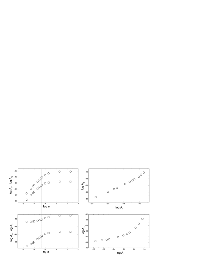
Figure 2: –Plots of $logA_{1}$ and $logA_{2}$ versus $\log\sigma$ (the left panels), and $logA_{2}$ versus $logA_{1}$ (the right panels) for a typical local pulse. In the two left panels, the open square and open circle represent $A_{1}$ and $A_{2}$, respectively, associated with a local pulse with an exponential rise and an exponential decay. Quantities $A_{1}$ and $A_{2}$ presented in the two upper panels represent the deviation of pulses from the standard decay form, and those in the two lower panels describe the deviation from the marginal decay curve. Other parameters are the same as those adopted in Fig. 1.

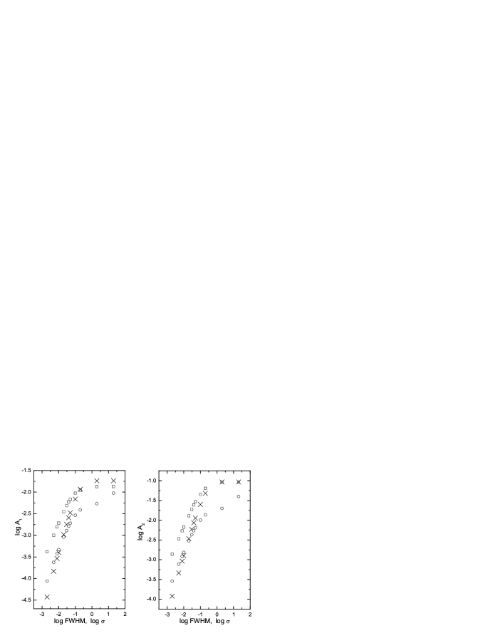
Figure 3: –Plots of $logA_{1}$ versus $logFWHM$ or $\log\sigma$ (the left panel), and $logA_{2}$ versus $logFWHM$ or $\log\sigma$ (the right panel) for some local pulses. Quantities $A_{1}$ and $A_{2}$ represent the deviation of the light curves associated with the local exponential decay pulse (the open square), the local power law decay pulse (with the power law index $\mu$=2) (the cross), and the local Gaussian pulse (the open circle), from the standard decay form. Other parameters are the same as those adopted in Fig. 1.

3 Decaying form seen in a FRED pulse sample

At least two questions urge us to employ a FRED pulse sample to make the following analysis. One is whether or not the reverse S-feature deviation characteristic indeed exists in the observed light curves, and the other is if the profiles of these light curves are indeed well below the marginal decay curve beyond the $FWHM$ position of the decay phase.

To study this issue, we utilize the light curves of the sample presented in Paper I, where the data are provided by the BATSE instrument on board the CGRO (Compton Gamma Ray Observatory) spacecraft. Of this sample, we find only the data of 75 individual pulses, which are employed in the following. It is well-known that pulses of a GRB show a tendency to self-similarity for each energy band (see, e.g. Norris et al. 1996). We thus consider in this paper only the light curve of channel 3 of BATSE, as signals in this channel are always significant.

The background of light curves is fitted by a polynomial expression using 1.024s resolution data that are available from 10 minutes before the trigger to several minutes after the burst. The data along with the background fit coefficients can be obtained from the CGRO Science Support Center (CGROSSC) at NASA Goddard Space Flight Center through its public archives. All of the background-subtracted light curves are fitted with equation (22) of Paper I, and then we normalize and re-scale the data of the background-subtracted light curves, using the method adopted above, with the corresponding fitting curves (the magnitude and $FWHM$ position of the background-subtracted light curves data could be well estimated from these fitting curves). We find that all pulses in our sample exhibit a reverse S-feature deviation from the marginal decay curve, where the (central) profiles of the light curves are indeed well below the marginal decay curve beyond the $FWHM$ position of the decay phase (see Figs. 4 and 5). When compared with the standard decay form, all of them except two, $\#$ 3257 and $\#$ 5495, show the reverse S-feature deviation as well (for the details see Fig. 5). A list of the deviation areas, $A_{1}$ and $A_{2}$, from the marginal decay curve and the standard decay form, are shown in Table 1, and their distributions are presented in Fig. 6.

Comparing Fig. 6 with Fig. 3 we find that for most pulses of the sample the widths of the decay phase of their corresponding local pulses are sufficiently large (larger than 0.1) that they are no more sensitive to the two areas $A_{1}$ and $A_{2}$. This suggests that, compared to the curvature delay time of the emitting region of the shock (see what discussed in last section), the intrinsic pulse decay times are long. This is because the FRED shape due to a local $\delta$-function pulse has a characteristic duration set by the curvature time delay — the time delay between the arrival times of two simultaneously emitted photons, one from the line-of-sight and one from $\theta_{max}$, but that due to a local pulse with a sufficiently long decay time has a different characteristic. At a certain observation time, only photons emitted from a limited area could reach the observer in the case of the local $\delta$-function pulse (in this case, the area could be marked by $\theta$ — $\theta+\Delta\theta$, when $\Delta\theta$ is extremely small), while in the case of the long decay time local pulse, photons emitted from all the areas concerned could be observed (they are emitted from different local times)(note that, in the case of the suddenly dimming local pulse, the corresponding area would decline with time). It seems that it is this difference that leads to the variance of the light curve characteristic seen in the two cases. Under this interpretation, we suspect that the fact that many BATSE pulses are in the saturation regime suggests that constraints may be placed on the angular size and radius of the emission region (which might deserve a further investigation).

Figure 4: –Plots of the observed light curves (the dot line) and the marginal decay curve (the solid line) for the 75 individual pulses of the sample.

Figure 5: –Plots of the fitting curves (the dot line), the standard decay form (the dash line) and the marginal decay curve (the solid line) for the 75 individual pulses of the sample.

Figure 6: Distributions of $A_{1}$ and $A_{2}$ of all the pulses in our sample. The two lower panels are associated with the marginal decay curve and the two upper panels correspond to the standard decay form (the two exclusive events are not included).

4 discussion and conclusions

A reverse S-feature deviation of profiles of light curves arising from local pulses containing a decaying tail from those associated with very narrow or suddenly dimming local pulses, the so-called standard decay form, could be seen in Fig. 3 of Paper II. We investigate in this paper if FRED pulses observed bear indeed this feature, and if they do how to measure the deviation. We define two areas $A_{1}$ and $A_{2}$ to describe the deviations within and beyond the $FWHM$ position in the decay phase, respectively. Suggested in our analysis, different from the standard decay form, there is a marginal decay curve which reflects the profile of the light curve arising from a local $\delta$ function pulse with a mono-color radiation. We employ a sufficiently large sample of FRED pulses of GRBs to study this issue. The study shows that the reverse S-feature indeed exists in the profiles of all the pulses concerned when compared with the marginal decay curve, while 73 out of 75 individual pulses show the feature as well when compared with the standard decay form. We also find that the values of $A_{1}$ and $A_{2}$ for most pulses of the sample are quite large which suggests that the corresponding local pulses might contain a long decay time relative to the time scale of the curvature effect.

For the two exclusive events, $\#$ 3257 and $\#$ 5495, the deviation from the standard decay form is “positive”, rather than “negative”, beyond the $FWHM$ position in the decay phase (say, $\tau^{\prime}>0.2$). We do not know what causes this exception. Here are several outlets we can think of. The first is associated with the background subtracting. We find that over or less subtracting the background count would shift the corresponding profile under or over the standard decay form beyond the $FWHM$ position in the decay phase. Illustrated in the left panel of Fig. 7 is this effect which is quite significant. The second is the impact of the rest frame radiation form. Note that the standard decay form is defined when the indexes of the rest frame spectrum are taken as $\alpha_{0}=-1$ and $\beta_{0}=-2.25$. As shown in Preece et al. (2000), the indexes could take many other values. We wonder if different values of the indexes could lead to a much different deviation. Shown in the right panel of Fig. 7 is this effect, where two modified standard decay forms, for which the rest frame spectral indexes of the standard decay form are replaced with others, are presented. It indicates that different values of the indexes could indeed change the profile beyond the $FWHM$ position in the decay phase, but the deviation is relatively small (compare the two panels of the figure).

Figure 7: The left panel is the plot of the effect of the background subtracting, on the deviation from the standard decay form, where the solid line is the standard decay form $C(\tau)$, the dash line represents the curve of $C^{\prime}(\tau)=C(\tau)+0.05C_{p}$ (which is associated with the case of less subtracting the background count), and the dot line stands for the curve of $C^{\prime}(\tau)=C(\tau)-0.05C_{p}$ (which corresponds to the case of over subtracting the background count). The right panel is the plot showing the effect of the rest frame radiation form on the deviation from the standard decay form, where the solid line is the standard decay form (for which, $\alpha_{0}=-1$ and $\beta_{0}=-2.25$ are adopted), the dash line is the modified standard decay form when replacing $\beta_{0}=-2.25$ with $\beta_{0}=-1$, and the dot line represents another modified standard decay form by replacing $\alpha_{0}=-1$ with $\alpha_{0}=-0.5$ and replacing $\beta_{0}=-2.25$ with $\beta_{0}=-4.5$.

As suggested in Paper II, equation (1) holds in the case of uniform jets. When $\theta_{\max}$ is very small (say, $\theta_{\max}\sim 1/\Gamma$), there will be a turnover feature in the decay tail of the light curve (see Paper II Fig. 2). One could check that, when $\theta_{\max}$ is sufficiently large, the turnover feature would not be detectable. In this case, a FRED pulse would also be observed. Therefore, the conclusion above holds as well in the case of uniform jets, as long as the opening angle of jets is not extremely small.

Hinted by our analysis and the previous works (see Ryde and Petrosian 2002; Paper II), one can conclude that the curvature effect would lead to FRED pulses, and for the pulses caused by the curvature effect their profiles would exhibit a reverse S-feature deviation from the marginal decay curve. Thus we propose to take the marginal decay curve as a criteria to check if an observed pulse could be taken as a candidate suffered from the curvature effect.

An interesting question arises accordingly, which is that, for those non-FRED pulses of GRBs, what one could expect. We suspect that, the reverse S-feature might no longer be observed in these cases and such pulses might be associated with structure jets or the scattering ejecta. This might deserve a further investigation (see Lu and Qin 2005 in preparation).

We thank the anonymous referee who located some errors in the original manuscript and made many helpful suggestions. This work was supported by the Special Funds for Major State Basic Research Projects (“973”) and National Natural Science Foundation of China (No. 10273019 and No. 10463001).

Table 1: A list of the estimated values of the deviation areas, $A_{1}$ and $A_{2}$, from the marginal decay curve and the standard decay form, for the pulses of our sample

trigger number	$A_{1}(M)$	$A_{2}(M)$	$A_{1}$	$A_{2}$	trigger number	$A_{1}(M)$	$A_{2}(M)$	$A_{1}$	$A_{2}$
563	0.0139	-0.162	0.0126	-0.0976	3648-3	0.0127	-0.123	0.0115	-0.0578
907	0.0119	-0.0993	0.0107	-0.0344	3765	0.0160	-0.180	0.0147	-0.115
914	0.0122	-0.108	0.0109	-0.0432	3870	0.00853	-0.0915	0.00723	-0.0266
973-1	0.0139	-0.140	0.0126	-0.0749	3875	0.00844	-0.136	0.00714	-0.0718
973-2	0.0133	-0.138	0.0120	-0.0735	3886	0.0133	-0.137	0.0120	-0.0723
999	0.0142	-0.146	0.0129	-0.0809	3892	0.014	-0.141	0.0127	-0.0766
1157	0.00941	-0.0786	0.00811	-0.0137	3954	0.0134	-0.144	0.0121	-0.0792
1406	0.00920	-0.0863	0.0079	-0.0214	4157	0.0125	-0.146	0.0112	-0.0811
1467	0.0140	-0.159	0.0127	-0.0936	4350-1	0.0168	-0.192	0.0155	-0.127
1733	0.0132	-0.144	0.0119	-0.0790	4350-2	0.00665	-0.135	0.00535	-0.0705
1883	0.0141	-0.148	0.0128	-0.0829	4350-3	0.0160	-0.186	0.0147	-0.122
1956	0.0154	-0.178	0.0141	-0.113	4368	0.0131	-0.128	0.0118	-0.0634
1989	0.0103	-0.0653	0.00896	-3.98E-4	5478-1	0.0153	-0.173	0.0140	-0.108
2083	0.0129	-0.132	0.0116	-0.0675	5478-2	0.0180	-0.201	0.0167	-0.136
2102	0.0135	-0.167	0.0122	-0.103	5495	0.00704	-0.00433	0.00574	0.0605
2138-1	0.0111	-0.0800	0.00976	-0.0151	5517	0.0143	-0.152	0.0130	-0.0878
2138-2	0.0106	-0.0895	0.00934	-0.0246	5523	0.0135	-0.171	0.0123	-0.107
2138-3	0.00789	-0.0660	0.00659	-0.00118	5541	0.0115	-0.112	0.0103	-0.0471
2193	0.0153	-0.180	0.0139	-0.115	5601	0.0136	-0.133	0.0123	-0.0690
2387	0.0165	-0.193	0.0152	-0.128	6159	0.0117	-0.149	0.0105	-0.0849
2484	0.0168	-0.194	0.0155	-0.129	6335	0.0118	-0.105	0.0105	-0.0406
2519	0.00525	-0.0845	0.00395	-0.0196	6397	0.0123	-0.106	0.0110	-0.0421
2530	0.0139	-0.173	0.0125	-0.108	6504	0.0158	-0.185	0.0145	-0.120
2662	0.00850	-0.134	0.0072	-0.0689	6621	0.0104	-0.0755	0.0091	-0.0107
2665	0.0117	-0.0949	0.0104	-0.0300	6625	0.0130	-0.168	0.0117	-0.104
2700	0.0130	-0.168	0.0117	-0.103	6672	0.0155	-0.170	0.0142	-0.106
2880	0.0129	-0.120	0.0115	-0.0547	6930	0.0178	-0.201	0.0165	-0.137
2919	0.0108	-0.09725	0.00945	-0.0323	7293	0.0117	-0.0937	0.0104	-0.0289
3003	0.0138	-0.142	0.0125	-0.0770	7295	0.00798	-0.121	0.00668	-0.0565
3143	0.0125	-0.136	0.0112	-0.0709	7475	0.0157	-0.174	0.0144	-0.109
3155	0.0144	-0.177	0.0131	-0.112	7548	0.0116	-0.0896	0.0103	-0.0248
3256	0.0153	-0.192	0.0140	-0.126	7588	0.0142	-0.168	0.0129	-0.103
3257	0.00816	-0.00482	0.00686	0.0683	7638	0.00709	-0.0704	0.00579	-0.00559
3290	0.00956	-0.0786	0.00826	-0.0137	7648	0.0167	-0.193	0.0154	-0.129
3415-1	0.00886	-0.130	0.00756	-0.0648	7711	0.0141	-0.152	0.0128	-0.0877
3415-2	0.0108	-0.157	0.00954	-0.0916	8049	0.0166	-0.185	0.0154	-0.121
3648-1	0.0138	-0.148	0.0125	-0.0827	8111	0.0105	-0.150	0.00926	-0.0855
3648-2	0.0144	-0.168	0.0130	-0.1032

Note: $A_{1}(M)$ and $A_{2}(M)$ are the two deviations of the profile of a light curve from the marginal decay curve.

References

- [Band et al. (1993)] Band, D.,Matteson, J., Ford, L., Schaefer, B., Palmer, D., Teegarden, B., Cline, T., Briggs, M., et al. 1993, ApJ, 413, 281
- [Fenimore et al. (1996)] Fenimore, E. E., Madras, C. D., and Nayakshin, S. 1996, ApJ, 473, 998
- [Fishman et al. (1994)] Fishman, G. J.,Gerald J., Meegan, Charles A., Wilson, Robert B., Brock, Martin N., Horack, John M., Kouveliotou, Chryssa, Howard, Sethanne, et al. 1994, ApJS, 92, 229
- [Fishman et al. (1995)] Fishman, G., Meegan, C. 1995, ARA&A, 33, 415
- [Ford et al. (1995)] Ford, L. A., Band, D. L., Matteson, J. L., Briggs, M. S., Pendleton, G. N., Preece, R. D., Paciesas, W. S., et al. 1995, ApJ, 439, 307
- [Friedman et al. (2001)] Friedman, Andrew S. and Bloom, Joshua S. 2005, APJ, 627, 1F
- [Fruchter et al. (1999)] Fruchter, A. S., Thorsett, S. E., Metzger, Mark R., Sahu, Kailash C., Petro, Larry, Livio, Mario, Ferguson, Henry, Pian, Elena, et al. 1999, APJ, 519,L13
- [Kocevski et al. (2003)] Kocevski, D., Ryde, F., and Liang, E. 2003, ApJ, 596, 389 (Paper I)
- [Lee et al.(2005)] Lee, A., Bloom, E. D., & Petrosian, V. 2000a, ApJS, 131,1
- [Lee et al. (2005)] Lee, A., Bloom, E. D., & Petrosian, V. 2000b, ApJS, 131, 21
- [Norris et al. (1996)] Norris, J. P., Nemiroff, R. J., Bonnell, J. T., Scargle, J. D., Kouveliotou, C., Paciesas, W. S., Meegan, C. A. and Fishman, G. J. 1996, ApJ, 459, 393
- [Piran (1999)] Piran, T. 1999, Phys. Rep., 314, 575
- [Preece et al. (1998)] Preece, R. D.,Pendleton, Geoffrey N., Briggs, Michael S., Mallozzi, Robert S., Paciesas, William S., Band, David L., Matteson, James L., Meegan, C. A. 1998, ApJ, 496, 849
- [Preece et al. (2000)] Preece, R. D., Briggs, M. S., Mallozzi, R. S., Pendleton, G. N., Paciesas, W. S. and Band, D. L. 2000, ApJS, 126, 19
- [Qin (2002)] Qin, Y.-P. 2002, A&A, 396, 705
- [Qin (2003)] Qin, Y.-P. 2003, A&A, 407, 393
- [Qin et al. 2004] Qin, Y. P., Zhang Z. B., Zhang F. W. and Cui X. H. 2004, APJ, 617, 439 (Paper II)
- [Ryde and Svensson (2002)] Ryde, F., & Svensson, R. 2000, ApJ, 529, L13
- [Ryde and Petrosian (2002)] Ryde, F., and Petrosian, V. 2002, ApJ, 578, 290
- [Schaefer et al. (1994)] Schaefer, B. E., Teegarden, Bonnard J., Fantasia, Stephan F., Palmer, David, Cline, Thomas L., Matteson, James L., Band, David L., Ford, Lyle A., et al. 1994, ApJS, 92, 285