HIGH ENERGY ASTROPHYSICAL PROCESSES

Abstract

We briefly review the high energy astrophysical processes that are related to the production of high energy $\gamma$-ray and neutrino signals and are likely to be important for the energy loss of high and ultrahigh energy cosmic rays. We also give examples for neutrino fluxes generated by different astrophysical objects and describe the cosmological link provided by cosmogenic neutrinos.

Bartol Research Institute, University of Delaware,
Newark, DE 19716, U.S.A.
E-mail: stanev@bartol.udel.edu

and

1 Introduction

The traditional high energy astrophysics is based purely on electromagnetic processes. Its recent extensions include the models for the production of TeV $\gamma$-rays, which are tested versus observations and proven to be conceptually correct. Such $\gamma$-rays are generated by the inverse Compton effect (ICE), in which accelerated electrons boost seed photons to the TeV energy range. Both basic types of ICE models: the synchrotron-self Compton model (SSC) and inverse Compton boosting of external photons can provide a good description of the observational data. In the SSC model seed photons are generated by synchrotron radiation of the accelerated electrons, which then boost them to high energy.

ICE models describe quite well the double peaked structure of the emission of AGN jets. The lower energy peak in the sub-MeV range represents the seed radiation, while the TeV peak is boosted by the accelerated electrons. The model parameters are also quite consistent with the high variability of the signals observed from active galactic nuclei (AGN), where the TeV $\gamma$-ray flux is known to double on the timescale of minutes. In addition, the SSC model gives a specific relation between the amplitudes of the TeV and sub-MeV signals, which is at least qualitatively similar to the observed one.

Neutrino astrophysics, on the other hand, is based on hadronic interactions that are not proven to happen in any astrophysical system. Defining the role of hadronic processes in the dynamics of powerful astrophysical systems is one of the aims of the neutrino astrophysics. There are though no reasons to believe that the observed TeV $\gamma$-ray signals are necessarily generated in purely electromagnetic processes and hadronic interactions have no contributions to them. Following the pioneering work in the last couple of decades there are now hadronic models that describe equally well the double peaked $\gamma$-ray energy spectrum. The lower energy photons are again generated by synchrotron radiation of electrons, but the electrons themselves are results of hadronic production of mesons and meson decays that feed electromagnetic cascades. The fast variability of the sources is more difficult to predict in hadronic models.

We shall discuss both types of processes. Neutrino producing processes include inelastic $pp$ and $p\gamma$ collisions, while the non-neutrino producing processes are the electromagnetic (Bethe–Heitler) $p\gamma$ interactions, $\gamma\gamma$ interactions, and the inverse Compton effect. Any astrophysical model has to include synchrotron radiation, which cannot be avoided in the relatively high magnetic fields that are needed to accelerate charged particles. Synchrotron radiation is the production process for sub-MeV photons, from $X$-rays down to radio waves.

We will not discuss particle acceleration. In principle, both protons and electrons should be accelerated to the same Lorentz factors in all astrophysical systems. Acceleration processes do not care about the particle charge. Injection, however, could be different. The injection of protons is better understood and described in detailed shock acceleration studies.

The same neutrino producing (and not producing) processes are important for the energy loss and propagational effects on ultra high energy cosmic rays (UHECR) in the microwave background (MBR) and in other radiation fields. Because the energy spectra of seed fields are quite different in different objects we will discuss the interaction lengths in the MBR, which provides the only standard photon field energy spectrum and allows for a reasonable comparison of different processes.

2 Neutrino producing processes

High energy astrophysical neutrinos are generated in the decay chains of mesons, such as $\pi^{\pm}\rightarrow\mu^{\pm}+\nu_{\mu}(\bar{\nu}_{\mu})$, $\mu^{\pm}\rightarrow e^{\pm}+\nu_{\mu}(\bar{\nu}_{\mu})+\nu_{e}(\bar{\nu}_{e})$. Other mesons are also involved to certain degree and all decay chains are very well known. What is not known is how the mesons are produced.

Inelastic $pp$ collisions are no doubt the best studied process in high energy physics. The proton interaction length in Hydrogen is 51 g/cm², shorter than the radiation length of 61 g/cm². For the average nucleon density in the Galaxy (1 cm^-3) this converts to a distance of 3$\times$10²⁵ cm, i.e. 10 Mpc, almost three orders of magnitude higher than the linear size of our Galaxy. If the Hydrogen target were a dense molecular cloud with density of 300 cm^-3 one interaction length would coincide with the diameter of the Galaxy. These numbers refer, of course, to the proton pathlength, and not directly to linear dimensions. Protons may be contained in magnetic fields, which will increase their interaction probability.

Because of the small average density of matter in astrophysics there are only a few objects that can present targets for $pp$ interactions. These are:

• stars

• accretion discs, that can contain column densities of 50 g/cm² close to the compact object, and

• dense molecular clouds, compressed, for example, by expanding supernova remnants. The density of such clouds can reach 1,000 cm^-3.

The disadvantage of the $pp$ collisions as important astrophysical process is in the rarity of the needed target material. The main advantage is the very low interaction threshold - a Lorentz factor of 1.3 for the production of the $\Delta$ resonance.

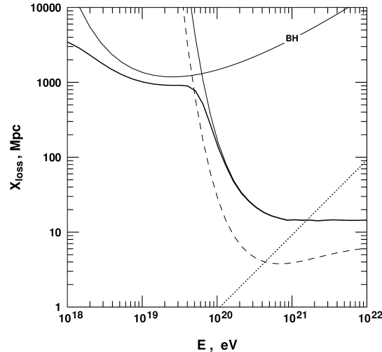
Figure 1: Energy loss length and protons in the microwave background.

Proton photoproduction is on the opposite end of interaction properties. Its main advantage is the availability of photon targets in all astrophysical systems, and even in extragalactic space. Only MBR has a number density in excess of 400 cm^-3 which fully compensates for the cross section ratio $\sigma_{p\gamma}/\sigma_{pp}$ which is of order 0.01. The main disadvantage of the photoproduction is its high energy threshold. The center of mass energy $E_{p}\epsilon(1-cos{\theta})$ should exceed the sum of the proton and pion masses squared. Since the photon background fields are often sub-eV this turns out to be a hard requirement.

Another difference between the two processes is the proton inelasticity coefficient $K_{inel}$ which describes the fractional energy loss of the proton in a collision. In inelastic $pp$ interactions $K_{inel}$ is about 0.5 and grows logarithmically with energy. In photoproduction interactions on the MBR $K_{inel}$ is 0.17 for protons of energy 10²⁰ eV, 0.27 at 10²¹ eV and only asymptotically approaches 0.5. The important astrophysical quantity $X_{loss}$, the energy loss length, equals $\lambda/K_{inel}$. At 10²⁰ eV it is almost a factor of six longer than the interaction length.

Figure 1 shows the energy loss length for protons in the microwave background. The dashed line is the interaction length for photoproduction $\lambda_{ph}$ and the thin solid lines show the $X_{loss}$ for photoproduction and for the Bethe-Heitler pair creation process. The thick solid line is the total $X_{loss}$ which also includes the adiabatic energy loss length of 4 Gpc for $H_{0}$= 75 km/s/Mpc.

The dotted line shows the neutron decay length. Only neutrons of energy exceeding 4$\times$10²⁰ eV undergo photoproduction interactions in the MBR. The neutron and proton photoproduction cross sections are almost identical, except at the energy threshold of the process. Lower energy neutrons always decay and generate $\bar{\nu}_{e}$, so one has to include neutron decay in the list of neutrino producing processes.

3 Electromagnetic processes

3.1 Pair creation by protons

The line marked BH shows the proton energy loss length in the electromagnetic pair creation process $p\gamma\rightarrow pe^{+}e^{-}$. This is an interesting process that may have a crucial importance for understanding the fate of ultrahigh energy cosmic rays (UHECR) in the Universe since it creates a feature in their spectrum ^?).

Figure 2: Energy spectra of positrons generated by protons of different energies in the MBR.

The proton energy loss in this process peaks at about 2$\times$10¹⁹ eV. The cross section of the process monotonically grows with the energy and the shape of the energy loss curve is determined by the decreasing proton inelasticity. $K_{inel}$ falls from 7$\times$10^-4 at 10¹⁸ eV to 10^-5 at 10²¹ eV. For this reason the electrons of the created pair have a similar energy distributions which is independent from the process cross section.

Figure 2 shows the spectra of the positrons generated in the MBR by protons of energy 10¹⁸, 10¹⁹, and 10²⁰ eV protons. Electron spectra are the same and the total energy loss is twice the integral of the histograms shown in Fig. 2.

The hardest electrons are generated by 10¹⁹ eV protons. For higher proton energies the electron spectrum is wider, but peaks at almost the same energy as at lower proton energy. The growing cross section can be visually detected by the increasing area of the histograms with the proton energy.

3.2 Inverse Compton scattering

Inverse Compton scattering is described by the same expressions as the Compton effect. High electrons interact with the seed photons and boost them to higher energy. The relation between the energies of the two particles is

$$k\;=\;{{\epsilon E_{e}}\over{m_{e}c^{2}}}\left(1-\beta cos{\theta}\right)$$

At low CM energies ($\epsilon E_{e}\ll(m_{e}c^{2})^{2}$) the process is in the Thomson regime which is characterized by the Thomson cross section $\sigma_{T}\;=\;8\pi r_{e}^{2}/3$ (665 mb) and a flat distribution of the boosted photons. At higher energy there is a transition to the Klein-Nishina regime during which the cross section decreases and the boosted photons become hard. Although the cross section decreases as $s^{-1/2}$ the interaction length may have a slightly different behavior as electrons interact on different parts of the seed photon spectrum. Asymptotically the boosted photon energy equals the electron energy.

3.3 Gamma-gamma collisions

In $\gamma$-ray producing environments inverse Compton scattering is always accompanied by the process $\gamma\gamma\;\rightarrow\;e^{+}e^{-}$ which is the opposite to electron–positron annihilation. The process cross section peaks at $s\;=\;4m_{e}^{2}$. In astrophysical settings the resonant behavior is less noticeable and the cross section peak is smoothed by the wide energy spectrum of the seed photons. Fig. 3 shows the interaction lengths for inverse Compton scattering and for pair production on the microwave background.

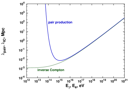
Figure 3: Interaction lengths for ICE (dots) and pair production by $\gamma\gamma$ collisions in the MBR.

At low energy one can see the ICE interaction length in the Thomson regime. The pair production process is below threshold in this energy range. It reaches its minimum interaction length at $E_{\gamma}$ = 1.20$\times$10⁶ GeV. Soon after that both cross sections start to decline at the same rate. As far as interactions in extragalactic space are concerned, the interaction lengths are modified by interactions on photon fields different from MBR. At energy lower than 10¹⁵ eV the infrared/optical background plays a major role. The observations of TeV $\gamma$-rays from distant AGN are often used to put limits on the density of the isotropic IR/O background in the near infrared region ^?,?). At energies above 10¹⁹ eV interactions on the radio background are important. Since the radio background in the MHz region is not observable, there is a large uncertainty in the $\gamma$-ray interaction length above 10¹⁹ eV. At still higher energy comes in the two pairs production process $\gamma\gamma\rightarrow e^{+}e^{-}\,e^{+}e^{-}$ which limits the $\gamma$-ray interaction length to 80 Mpc even in the absence of radio background.

The similar cross sections of these two processes and their small interaction lengths support the development of electromagnetic cascades in astrophysical objects and in the extragalactic space. Photons interact to produce $e^{+}e^{-}$ pair. Electrons then scatter the seed photons to high energy and the scattered photons generate another pair. At high energy, when both ICE and pair production interactions have high energy transfer, i.e. the secondary particles have almost the same energy as the interacting ones, the cascade development leads only to a slow degradation of the initial $\gamma$-ray energy. Close to the $\gamma\gamma$ energy threshold the pair electron distribution becomes more uniform and the energy degradation speeds up.

The major contributor to the acceleration of these electromagnetic cascades is the synchrotron radiation that high energy electrons suffer in the presence of magnetic fields.

3.4 Synchrotron radiation

Synchrotron radiation (magnetic bremsstrahlung) is a very important energy loss process for charged particles in the presence of magnetic fields. The energy loss is proportional to the electron Lorentz factor squared times the energy density of the magnetic field and depends on the pitch angle of the electron with the magnetic field lines. For an ensemble of relativistic electrons that are scattered randomly in all directions the energy loss averaged over all pitch angles in particle physics units is

$$-{{dE}\over{dt}}\,=\,3.79\times 10^{-6}\left({{B}\over{{\rm Gauss}}}\right)^{2}\left({{E_{e}}\over{{\rm GeV}}}\right)^{2}\;{\rm GeV/s}\;.$$

The characteristic frequency of the radiated photons is their critical frequency

$$\nu_{c}\,=\,1.61\times 10^{13}\left({{B}\over{{\rm Gauss}}}\right)\left({{E}\over{{\rm GeV}}}\right)^{2}\,{\rm Hz}\;.$$

Expressed as a fraction of the electron energy the critical frequency is proportional to the product of the energy and the magnetic field value $\nu_{c}\propto E_{e}^{2}\times B$. The number of emitted photons peaks at 0.29$\nu_{c}$. The higher the energy, the harder is the spectrum of the radiated photons as illustrated in Fig. 4.

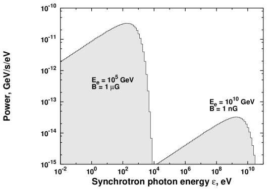
Figure 4: Synchrotron photon power for 10¹⁴ eV electrons in 1 $\mu$G field (left) and for 10¹⁰ eV electrons in 1 nG field.

The total energy loss of a 10¹⁹ eV electron in 10^-9 G field is higher than that of a 10¹⁴ eV electron in $\mu$G field by 10⁴, but the critical frequency of the photons it emits is higher by 10⁷. Note that synchrotron radiation brings the energy of the 10¹⁹ eV electron directly into the GeV range.

Since the synchrotron energy loss depends on the square of the particle Lorentz factor it is thus inversely proportional (for the same total energy) to the square of the particle mass. A proton loses only $(m_{e}/m_{p})^{2}\simeq 3\times 10^{-7}$ times as much energy as an electron of the same $E_{tot}$. The energy loss of muons is 2.37$\times$10^-5 down from the electron one for the same energy. Proton and muon energy losses on synchrotron radiation can thus be important only in very strong magnetic fields and respectively higher particle energy.

Figure 5 compares the proton energy loss length to the photon $\gamma\gamma$ interaction length (which can be considered energy loss length in the presence of magnetic field) in the microwave background. The radio background ^?) is included in the calculation of the photon interaction length. Because of that the energy loss distances for the highest energy photons are still highly uncertain.

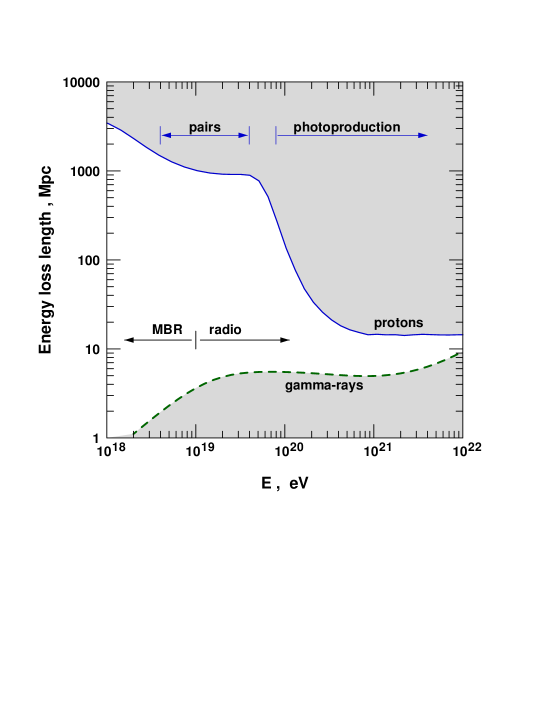
Figure 5: The energy loss length for protons in MBR is compared to the photon energy loss length.

Electromagnetic processes lead to faster energy loss for high energy photons and electrons than nucleons lose in hadronic interactions. The actual interaction rates, however, depend strongly not only on the total energy density of the seed radiation, but also on its energy spectrum. Since all particle production processes have energy thresholds, and only the seed photons above that threshold count, different environments could favor electromagnetic or hadronic processes as demonstrated in ^?) in the case of BL Lac objects.

The immediate conclusion from this brief review is that all physics processes are very well known, and the main uncertainties in our estimates come from the lack of knowledge on the astrophysical environments in potential neutrino sources.

4 Resonant neutrino cross sections

It will be a loss not to mention a couple of resonant neutrino cross sections that have never been measured, but have been calculated on a solid physics basis.

Figure 6: Left hand panel: cross section for the ‘Glashow’ resonance, shown with one of its extensions. Right hand panel: neutrino annihilation, and resonant neutrino-photon interaction. The $\nu\gamma$ cross section does not depend on the neutrino mass.

The one shown in the left hand panel of Fig. 6 is the resonant interaction of $\bar{\nu}_{e}$ with electrons, that was suggested by Glashow ^?). The idea was developed to its current understanding by Berezinsky & Gazizov ^?). The cross section peaks at $E_{\bar{\nu}_{e}}\;=\;M_{W}^{2}/(2m_{e})\;=$ 6.4$\times$10⁶ GeV. The maximum value including all nine $W^{-}$ decay channels is 4.7$\times$10^-31 cm². There are numerous extensions the resonant $\bar{\nu}_{e}e^{-}$ scattering. We show one of them, $\bar{\nu}_{e}e^{-}\rightarrow\gamma W^{-}$, that enhanced the width of the resonance to higher neutrino energy ^?).

The right hand panel shows the neutrino annihilation ($\nu\nu\rightarrow Z_{0}$) cross section which peaks at energy $Z_{0}^{2}/m_{\nu}$. It is plotted for $m_{\nu}$ = 1 eV. This process has been used as a basis of the Z-burst scenario for the ultrahigh energy cosmic rays, where UHECR are result of $Z_{0}$ decay within the GZK sphere of about 50 Mpc ^?,?). The cross section for the process $\nu\gamma\rightarrow e^{-}W^{+}$ (right hand panel) does not depend on the neutrino mass but it does depend on the lepton mass. In the contemporary universe it peaks at neutrino energy about 10¹⁶ GeV and is totally insignificant. It does, however, lead to absorption of all high energy neutrinos generated at high redshifts. The influence of this process is felt already at ($z\;>\;$10) in interactions on the MBR ^?).

5 Examples of predicted neutrino fluxes

We do not have the ambition to review the models for the production of high energy astrophysical neutrinos in this talk. The discussion of the relevant processes would be, however, not complete without several examples of predicted fluxes.

5.1 Source neutrinos

Figure 7 shows $\nu_{\mu}+\bar{\nu}_{\mu}$ fluxes predicted for five potential neutrino sources. The atmospheric neutrino fluxes within 1^∘ from the source are indicated with a shadowed region. The upper edge of that region corresponds to horizontal neutrinos and lower one - to vertical neutrinos.

The curve labeled 1) shows the neutrinos that we expect from the direction of the Sun ^?). High energy neutrinos are generated by cosmic ray interactions in the rarefied solar envelope and some of them propagate through it to us. The energy spectrum of these neutrinos is flatter than the one of atmospheric neutrinos because mesons decay easier in the tenuous environment.

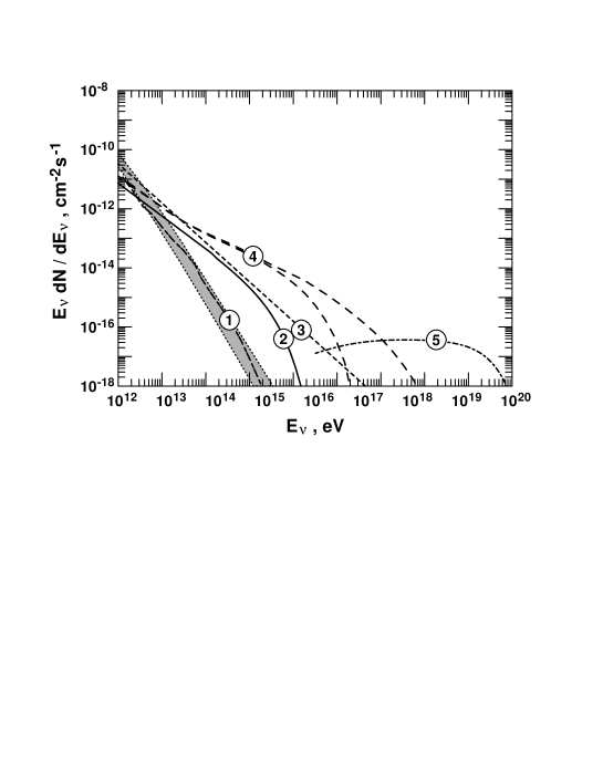
Figure 7: Examples of several different source neutrino fluxes. See text for a brief description of the models.

The second curve shows the neutrino fluxes expected from the supernova remnant IC443 if the $\gamma$–rays detected by EGRET ^?) are all of hadronic origin ^?). The neutrino flux does not reach very high energy because the EGRET detection is consistent with a low maximum energy for the accelerated cosmic rays. The detected $\gamma$-ray fluxes should be generated in hadronic interactions if the accelerated protons hit a dense molecular cloud ($>$300 cm^-3) or are contained in a more tenuous cloud by magnetic fields.

Neutrinos in these first two examples are generated in $pp$ interactions while the next three models are based on photoproduction. Curve 3) shows the expected neutrino luxes if the TeV $\gamma$-ray outburst of Mrk 501 ^?) is of hadronic origin. The neutrino flux extends to higher energy than the detected $\gamma$-rays as the latter may have been absorbed in $\gamma\gamma$ collisions either on source or in propagation to us.

Curve 4) shows the minimum and maximum fluxes expected from the core region of 3C273 ^?). The photon density in the core region is estimated from the total luminosity of the source and the proton density is estimated from the accretion rate that could support the source luminosity. Magnetic field (estimated by equipartition) is sufficient for the acceleration of protons to high energy. Since the photon density exceeds the proton density by at least eight orders of magnitude, photoproduction is the major energy loss process for the high energy protons.

Curve 5) shows the neutrino flux predicted for the jet of 3C279 ^?). Neutrinos are boosted to higher energy by the Doppler factor of the jet, which is 10 in this example.

There are obviously many more, and newer, models, but the selection shown above includes examples of all possible types of astrophysical objects that are potential neutrino sources. There are also galactic models that rely on photoproduction interactions in objects like micro-quasars.

5.2 Diffuse neutrinos

Figure 8 shows several different diffuse astrophysical neutrino fluxes. The shaded area indicates the vertical and horizontal fluxes of atmospheric neutrinos. The Waxman&Bahcall limit ^?). derived from the flux of the highest energy cosmic rays in optically thin astrophysical objects is indicated with W&B.

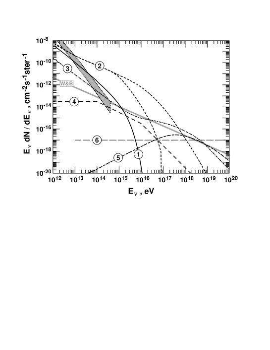
Figure 8: Examples of several diffuse neutrino fluxes. See text for a brief description of the models.

The curve labeled 1) shows the neutrinos expected from the central Galaxy in the assumption that all diffuse $\gamma$-rays detected by EGRET ^?) are created by cosmic ray interactions with matter. This is indeed a standard assumption for photons of energy above 100 MeV. The only questionable feature of this observation is that the $\gamma$-ray energy spectrum is flatter than what is expected from interactions of the locally observed cosmic rays. This can be assigned to the existence of unresolved sources with spectra much flatter than those of the local cosmic rays.

Curves 2) come from a cosmological integration of the models of Ref. ^?). The cosmological evolution of AGN is assumed to be close to $(1+z)^{4}$ (although the form used is much more sophisticated). Since the AGN cores are optically thick these fluxes do not have to obey the W&B limit.

Flux 3) is the isotropic AGN neutrino flux from Ref. ^?), where $pp$ interactions are added to the high energy photoproduction interactions. For about two decades(10^16.5 - 10^18.5 eV) the flux exceeds the W&B limit by a small amount. The neutrino flux from $pp$ interactions does not have to obey the limit.

Flux 4) is the prediction of diffuse neutrinos from gamma ray bursts ^?) in the assumption that GRBs are sources of the ultrahigh energy cosmic rays.

Flux 5) is a nominal cosmogenic neutrino flux as calculated in Ref. ^?) using the luminosity and cosmological evolution model from the W&B limit.

Finally, for comparisons with diffuse astrophysical neutrinos we show the neutrino flux (label 6)) that is needed by the Z-burst model to become the production mechanism for UHECR ^?).

6 Cosmogenic neutrinos and cosmological evolution of the astrophysical sources

Cosmogenic neutrinos are generated by photoproduction interactions of high energy cosmic rays, mostly with the microwave background ^?,?). To illustrate the strong cosmological link we shall build a model of the production of cosmogenic neutrinos, that includes the following simplifying assumptions following Ref. ^?):

• The microwave background is the only target for cosmic ray interactions.

• The Universe is matter dominated ($\Omega_{M}$ = 1).

• Neutrino production is very fast on cosmological scale.

• Cosmic ray sources evolve as $(1+z)^{m}$ forever.

The simplicity of the model changes the result of the calculation by less than a factor of two.

The neutrino yield $Y$ from protons of energy $E_{p}$then scales with the redshift as $E_{\nu}\frac{dY}{dE_{\nu}}(E_{\nu},E_{p},z)=E_{\nu}\frac{dY_{0}}{dE_{\nu}}(q^{2}E_{\nu},qE_{p})\;,$ where $Y_{0}$ is the yield in the contemporary universe and $q=1+z$. To obtain the flux of atmospheric neutrinos one can integrate over $E_{p}$ and $\ln{q}$ and obtains

$$E_{\nu}\frac{d\Phi}{dE_{\nu}}(E_{\nu})=\frac{A}{H_{0}}\int_{0}^{q_{max}}d(\ln q)q^{(m+\gamma-\frac{3}{2})}E_{\nu}\frac{dY_{0\gamma}}{dE_{\nu}}(q^{2}E_{\nu})\;,$$

where the yield $Y_{0\gamma}$ depends on the integral slope of the cosmic ray injection spectrum $\gamma$.

The interesting result here is the $q^{(m+\gamma-\frac{3}{2})}$ dependence of the flux, when the result is expressed in an integral over $\ln{q}$. For $(m+\gamma)$ less than 1.5 the contribution to the cosmogenic neutrino flux decreases with redshift. If $(m+\gamma)$ = 1.5 the contribution of all cosmological epochs is exactly the same. We assumed $\Omega_{M}$ = 0 to show this flat contribution. In a $\Lambda$ dominated Universe a slight curvature would appear. For values higher than 1.5 earlier cosmological epochs dominate the flux as shown in Fig. 9.

Figure 9: Cosmogenic neutrino fluxes from the simplified model described above. The thin lines show the contributions to the total flux from redshifts $z$ = 0, 1, 2, … 10, from right to left. The points show the total flux.

For higher values of ($m+\gamma$) the contribution of earlier cosmological epochs would be so strong that they would dominate even when a more reasonable source evolution model (with a cut-off) is used. The total flux of cosmogenic neutrinos also significantly increases.

This is directly related to the fits of the extragalactic cosmic ray spectrum. There are generally two types of fits:
Scenario 1: A steep cosmic ray injection spectrum ($\gamma>$ 1.5) after propagation fits well the measured spectrum down to 10¹⁸ eV. The second knee ^?) of the spectrum, a dip in the spectral shape when multiplied by $E^{3}$, is due to the BH pair production by protons as predicted in ^?). The shape of the propagated spectrum is such that no cosmological evolution of the cosmic ray sources is possible.
Scenario 2: The injection spectrum is flat ($\gamma$ = 1) as expected from shock acceleration models. Since a flat injection spectrum can not fit the measured cosmic ray spectrum, a cosmological evolution of the cosmic ray sources of order $(1+z)^{3}$ is needed. Even then the galactic cosmic ray spectrum has to extend up to 10¹⁹ eV. The second knee is formed at the intersection of the galactic and extragalactic cosmic ray spectra.

Both scenarios have been discussed quite actively in the literature during the recent couple of years. Each one has its supporters, although for now this is only a matter of preference. Scenario 1 has been presented in ^?,?,?) and discussed in other recent publications. Scenario 2 was developed in ^?) and supported in ^?) and elsewhere. One difference between these two scenarios is the flux of cosmogenic neutrinos that they generate in the assumption of uniform and heterogeneous distribution of cosmic ray sources. In the case of Scenario 1 the sum $\gamma+m$ is 1.7, while in Scenario 2 the sum is 4. Scenario 2 will thus generate much larger flux of cosmogenic neutrinos than Scenario 1.

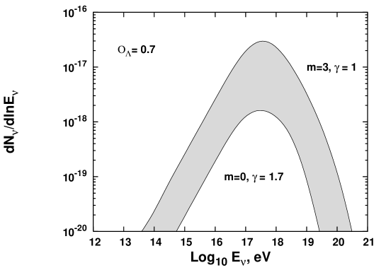
Figure 10: Cosmogenic neutrino fluxes generated by the two scenarios for the detected flux of UHECR. The $\gamma,m$ values are indicated in the graph.

Figure 10 shows the cosmogenic neutrino spectra from these two scenarios for the cosmic ray emissivity of 4.5$\times$10⁴⁵ ergs/Mpc³/yr that was derived by Waxman ^?). Cosmological model with $\Omega_{M}$ = 0.3 and $\Omega_{\Lambda}$ = 0.7 was used for this calculation. The actual difference between the models could be a bit smaller since Scenario 1 requires higher emissivity.

There are also other difference between the two scenarios. The main one is that the transition between galactic and extragalactic cosmic rays is earlier (at smaller energy) by one order of magnitude in Scenario 1. Since we presume that galactic cosmic rays at that energy are all heavy nuclei (iron) they produce different energy dependence of the cosmic ray chemical composition. The Auger Southern Observatory will hopefully measure the composition with smaller ambiguity than exists today, it will help to solve the problem. So would the detection of the cosmogenic neutrino fluxes by the current planned and constructed neutrino detectors. ANITA, IceCube, Mediterranean km³, RICE) may confirm the existence of GZK neutrinos. A next generation of experiments (EUSO, OWL, SalSA, X-RICE) is being planned which would provide sufficient statistics (10-100 GZK events per yr) to complement and expand the AUGER observations. Successful completion of one such experiment would be an important step toward understanding the sources of the highest energy particles in the Universe.

Acknowledgments. The author acknowledges helpful discussions with V.S. Berezinsky, P.L. Biermann, T.K. Gaisser, D. DeMarco, D. Seckel and other colleagues. This research is supported in part by the US Department of Energy contract DE-FG02 91ER 40626 and by NASA Grant NAG5-10919. The possibility to participate in the Venice Workshop on Neutrino Telescopes and the excellent content and organization of the meeting is highly appreciated.

References

- [1] V.S. Berezinsky & S.I. Grigoreva, Astron. Astrophys.,199, 1 (1988)
- [2] M.H. Salamon & F.W. Stecker, ApJ, 493, 547 (1998)
- [3] T. Stanev & A. Franceschini, ApJ., 494, L159 (1998)
- [4] R.J. Protheroe & P.L. Biermann, Astropart. Phys.,6, 45 (1996)
- [5] A. Mücke et al., Astropart. Phys., 18, 593 (2003)
- [6] S. Glashow, Phys. Rev., 118, 316 (1960)
- [7] V.S. Berezinsky & A.Z. Gazizov, Pisma Zh. Eksp. Theor. Phys. 25, 276 (1977), JETP Lett. 25, 254 (1977)
- [8] D. Seckel, Phys. Lett. Lett.,80, 900 (1998)
- [9] T. Weiler, Astropart. Phys., 11, 303 (1999)
- [10] D. Fargion, B. Mele & A. Salis, ApJ, 517, 725 (1999)
- [11] D. Seckel, T. Stanev & T.K. Gaisser, ApJ, 382, 652 (1991)
- [12] J.A. Esposito et al., ApJ, 461, 820 (1996)
- [13] T.K. Gaisser, R.J. Protheroe & T. Stanev, ApJ,492, 219 (1998)..
- [14] see, e.g. F. Aharonian et al., A&A, 327 L5 (1997) for the highest energy -ray observation
- [15] A.P. Szabo & R.J. Protheroe. Astropart. Phys., 2, 375 (1994)
- [16] K. Mannheim, T. Stanev & P.L. Biermann, A&A, 260, L1 (1992)
- [17] E. Waxman & J.N. Bahcall, Phys. Rev., D59:023002 (1999)
- [18] S.D. Hunter et al., ApJ, 481, 205 (1997)
- [19] K. Mannheim, Astropart. Phys.,3, 295 (1995)
- [20] E. Waxman & J.N. Bahcall, Phys. Rev. Lett., 78, 2292 (1997)
- [21] R. Engel, D. Seckel & T. Stanev, Phys. Rev. D64:093010 (2001)
- [22] D.V. Semikoz & G. Sigl, JCAP, 04, 3 (2004)
- [23] V.S. Berezinsky & G.T. Zatsepin, Phys. Lett. 28b, 423 (1969); Sov. J. Nucl. Phys. 11, 111 (1970)
- [24] F.W. Stecker, Astroph. Space Sci. 20, 47 (1973)
- [25] D. Seckel & T. Stanev, astro-ph/0502XXX
- [26] R.U. Abbasi et al., (HiRes Collaboration), astro-ph/0407622.
- [27] V.S. Berezinsky, A.Z. Gazizov & S.I. Grigorieva, astro-ph/0204357; astro-ph/0210095
- [28] R. Aloisio & V.S. Berezinsky, astro-ph/0412578
- [29] M. Lemoine, astro-ph/0411173
- [30] E. Waxman & J.N. Bahcall, Phys. Lett. B 226, 1 (2003)
- [31] T. Wibig & A.W. Wolfendale, astro-ph/0410624
- [32] E. Waxman, Ap. J. 452, L1 (1995)