Three-dimensional modeling of Type Ia supernovae - The power of late time spectra

Late time synthetic spectra of Type Ia supernovae, based on three-dimensional deflagration models, are presented. We mainly focus on one model, “c3_3d_256_10s”, for which the hydrodynamics (Röpke 2005) and nucleosynthesis (Travaglio et al. 2004) was calculated up to the homologous phase of the explosion. Other models with different ignition conditions and different resolution are also briefly discussed. The synthetic spectra are compared to observed late time spectra. We find that while the model spectra after 300 to 500 days show a good agreement with the observed Fe II-III features, they also show too strong O I and C I lines compared to the observed late time spectra. The oxygen and carbon emission originates from the low-velocity unburned material in the central regions of these models. To get agreement between the models and observations we find that only a small mass of unburned material may be left in the center after the explosion. This may be a problem for pure deflagration models, although improved initial conditions, as well as higher resolution decrease the discrepancy. The relative intensity from the different ionization stages of iron is sensitive to the density of the emitting iron-rich material. We find that clumping, with the presence of low density regions, is needed to reproduce the observed iron emission, especially in the range between 4000 and 6000 Å. Both temperature and ionization depend sensitively on density, abundances and radioactive content. This work therefore illustrates the importance of including the inhomogeneous nature of realistic three-dimensional explosion models. We briefly discuss the implications of the spectral modeling for the nature of the explosion.

1 Introduction

During the past few years Type Ia supernovae (SNe Ia) have become the main tool to measure the expansion rate of the Universe with the surprising result that it is presently in a phase of accelerated expansion. The importance of SNe Ia as distance indicators comes from the fact that they are bright and can be observed at large distances. Moreover, the homogeneity of their observable properties, such as light curves and spectra, makes it reasonable to calibrate the light curves in such a way that they become “standard candles”. In fact, empirical recipes to perform the calibration have been very successful. Today, by decreasing the statistical errors by the rapidly increasing number of observed SNe Ia at intermediate and high redshifts, attempts are made to constrain also the equation of state of the “dark energy” that is thought to be the cause of the acceleration.

However, in any such studies it is important to understand the systematic errors, which are here likely to dominate. The intrinsic dispersion, i.e. originating from properties of the explosions cannot be controlled by observing a large number of SNe Ia. We therefore here compare realistic models to detailed observations to get a better understanding of the physics leading to the homogeneity of the observed properties, and the inherent uncertainties.

The presently favored model for a Type Ia supernova is the thermonuclear explosion and disruption of an accreting carbon-oxygen white dwarf with a mass close to the Chandrasekhar limit. Guided by the presence of intermediate-mass elements in the observed spectra these models assume that thermonuclear burning begins as a (subsonic) deflagration, which may or may not change into a (supersonic) detonation at later times. Recently, there has been great progress in the modeling of such explosions by means of combustion-hydrodynamics codes. In particular, three-dimensional deflagration calculations of increasing complexity have been performed by a number of groups, Reinecke et al. (2002a, 2002b), Gamezo et al. (2003) and Garcia-Senz & Bravo (2005). Although there are rather large differences in the ways turbulent thermonuclear flames are modeled by the groups, they arrive at similar conclusions, namely that the chemical structure of the supernova should be highly inhomogeneous. In particular, they find substantial amounts of unburned carbon and oxygen close to the center. Whether this is a result of inadequate modelling of the nuclear burning, or is a real feature can best be decided by comparing model spectra with observations.

In this paper we demonstrate the possibility of testing the multidimensional hydrodynamics and nucleosynthesis calculations by studying the late time spectra. The emission at late times, i.e. later than $\sim$ 100 days, is predominantly emerging from the central parts of the supernova, where the effects of the explosion are most pronounced. Therefore, by comparing model spectra, based on different explosion models, to observations one can draw conclusions about the explosive nucleosynthesis, hydrodynamic mixing, the amount of ⁵⁶Ni formed, and the total energy of the explosion. In contrast, early spectra are more sensitive to the chemical structure of the high velocity outer regions. The two phases therefore nicely complement each other. The input models used in this study come from the calculations by Travaglio et al. (2004), who have made a detailed post processing nucleosynthesis of the hydrodynamic models by Reinecke et al. (2002a, 2002b) and Röpke (2005). The hydrodynamic code only had a minimal nucleosynthesis network included, sufficient for a good approximation of the thermonuclear energy release.

In section 2 we first summarize the three-dimensional hydrodynamical models and the nucleosynthesis we use as input to our spectral code. Then we discuss the late-time spectral modeling. Our results are given in section 3. In section 4 we discuss our findings, and what we can learn from late time spectra. Finally in section 5 we summarize our results.

2 Modeling

2.1 3D hydrodynamical modeling

Our input models for the spectral-synthesis code come from the multidimensional hydrodynamic calculations of Reinecke et al. (2002a, 2002b). In order to save computer time with still sufficient numerical resolution, only an octant of the star was simulated and mirror symmetry was assumed at the inner boundaries. This artificial symmetry causes some problems with the shapes of the emission lines of the nebular spectra, as will be discussed later. Recently Röpke (2005) has evolved one of their three-dimensional explosion models up to 10 seconds, at which time the assumption of homologous expansion is valid.

The simulations of Reinecke et al. (2002a, 2002b) attempt to model the nuclear burning and hydrodynamics from first principles, as far as possible. The nuclear burning is modeled as a subsonic, turbulent deflagration. Because the length scales vary from sub-mm scales to dimensions comparable to the radius of the white dwarf, some simplifying assumptions about the physics of the flame front on small length scales have to be invoked. The first assumption is that since the flamefront cannot be numerically resolved it is replaced by a sharp discontinuity between “fuel” and “ashes”. This discontinuity is then modeled by a level-set function. The remaining unknown is the normal velocity of the level set, i.e. the turbulent flame speed. Since in the flamelet regime of turbulent combustion (valid for Type Ia supernovae down to densities of around 10⁷ g cm^-3) the flame velocity is independent of the physics on microscopic scales, it can be determined from a sub-grid scale model of the unresolved turbulent velocity fluctuations. These, in turn, result from a Kolmogorov-like turbulent cascade with energy fed in by large-scale hydrodynamic instabilities, predominantly the Rayleigh-Taylor (buoyancy-driven) instability. The important parameters determining the evolution of the explosion are the central density and the composition of the white dwarf. All simulations used in the present study started with a central density of $2.9\times 10^{9}\rm\leavevmode\nobreak\ g\leavevmode\nobreak\ cm^{-3}$ and equal carbon and oxygen mass fractions.

The numerical experiments in Reinecke et al. (2002a, 2002b) show that the way the explosion is initiated can have large effects on the outcome, especially on the explosion energy and the ⁵⁶Ni mass. This is likely to be determined by the evolution leading up to the ignition. According to Garcia-Senz & Woosley (1995) possible ignition conditions could be a couple of floating “blobs” of burning material accelerated to a fraction of the sound velocity near the center of the star. Alternatively, large scale convective motions could lead to ignition in extended regions at the center (Höflich & Stein 2002), or a multi-point ignition with an exponentially increasing and asymmetric number of ignition points out to approximately 150 – 200 km off-center (Woosley, Wunsch & Kuhlen 2004).

In the simulations by Reinecke et al. the effects of the ignition were explored by assuming different ignition topologies. In particular, in one set of models the explosion is initiated at the center, while in a second set of calculations the explosion starts in a finite number of randomly distributed, floating bubbles. The result of this is that the more complex the initial conditions are, the more ⁵⁶Ni seems to form and the stronger the explosion energy. This is not too surprising because, in general, a more complex geometry has a larger surface area, increasing the burning rate and leading to a higher energy. Also, the amount of unburned carbon and oxygen that is dredged-down to the center between the rising Rayleigh-Taylor blobs depends on the geometry of the ignition region, but this effect has not yet been fully explored.

Finally, the numerical resolution is important, mostly for the nucleosynthesis but, to a lesser extent also for the kinetic energy of the explosion. This is especially important for the mass of ⁵⁶Ni produced and also the amount of unburned carbon and oxygen near the center of the star, and both are crucial parameters for the calculations of synthetic spectra. The reason can easily be understood. For instance, the number of initial burning blobs is limited by the number of grid points. Low resolution means few blobs with rather large sizes, in contrast to the few kilometers expected from analytical models (Woosley, Wunsch & Kuhlen 2004). These large blobs rise fast and burn little fuel, leaving behind lots of unburned gas. In contrast, high resolution allows for more realistic initial conditions and thus for more burning early on in the explosion. Similar arguments hold for other initial conditions. The further evolution, however, is much less affected because once turbulence has developed the subgrid-scale model takes care of resolution effects. Resolution studies underway (Röpke & Hillebrandt 2005c) seem to indicate that even computations with (static) grids of 512³ mesh points may not describe the early evolution correctly as far as the nucleosynthesis yields are concerned. We will come back to this question later.

In the present paper we will use three different 3D models, referred to as b30_3d_768, b5_3d_256, and c3_3d_256. In Table 1 we summarize the main characteristics of the different hydrodynamical models studied here. The label c3 refers to central burning, while b30 and b5 refer to models, where the burning starts in 30 and 5 blobs, respectively. The last number refers to the resolution of the model, in theses cases $768^{3}$ or $256^{3}$ grid points, respectively. While the b5_3d_256, and c3_3d_256 are from Reinecke et al. (2002b), the high resolution model b30_3d_768 is discussed in Travaglio et al. (2004). From what we discussed in the previous paragraph it is obvious that the nuclear abundances obtained from the models with low numerical resolution need to be considered with caution.

The calculations by Reinecke et al. (2002b) follow the explosion up to 1.2 – 1.5 seconds. After that time the outermost layers are ’escaping’ their fixed Eulerian grid. However, a problem for any spectral modeling is that the ejecta have at that time not yet reached homologous expansion, but the velocities and densities are still affected by pressure and gravity. This problem has recently been solved by Röpke (2005), who calculated the hydrodynamics for the c3_3d_256 model by Reinecke et al. (2002b) up to 10 seconds after the explosion, using a moving grid. We will in this paper refer to this model as c3_3d_256_10s. At 10 seconds the ejecta are indeed moving homologously, and have reached their final velocities and densities. In this paper we will mainly concentrate on the c3_3d_256_10s model, and just briefly discuss the models b30_3d_768, c3_3d_256 and b5_3d_256 with respect to the initial conditions and resolution.

The kinetic energies for the models are given in Table 1. These energies all refer to the end of the simulations, i.e. at 1.2 – 1.5 s. However, as shown by Röpke (2005), the kinetic energy does not change much between 1.5 s and 10 s. The maximum velocity for the tracer particles (and the supernova ejecta) in the c3_3d_256_10s model is roughly $\sim 12800\rm\leavevmode\nobreak\ km\leavevmode\nobreak\ s^{-1}$.

2.2 Nucleosynthesis calculations

Travaglio et al. (2004) have calculated the nucleosynthesis based on the hydrodynamical models in Reinecke et al. (2002a, 2002b). The nucleosynthesis calculations for the multidimensional explosion models are discussed in detail in Travaglio et al. . Here we just summarize the main features. For computational reasons the hydrodynamical models of the explosions only include a few representative nuclei (⁴He, ¹²C, ¹⁶O, ²⁴Mg and ⁵⁶Ni) in a simplified reaction network, sufficient to calculate the nuclear energy release. This is, however, not sufficient for more detailed spectral models, or for a detailed comparison of the nucleosynthesis. Therefore, a post-processing step with a full nucleosynthesis network was performed, with the physical conditions of ’tracer particles’ as input.

The reason for introducing such tracer particles is the need to map the Eulerian hydrodynamics grid onto a Lagrangian grid for the nucleosynthesis computations. Therefore in the hydrodynamics a number of tracer particles are followed, recording the temperature and density as a function of time, sufficiently large to represent the matter of the exploding star. Technically this is done by subdividing the star into a Cartesian grid of ($27^{3}=19683$) cells, equidistant in the integrated mass, azimuthal angle $\phi$ and cos$\theta$ such that all cells contain the same mass: 1.39 M_⊙/19683 = $7\times 10^{-5}$ M_⊙. A tracer particle is placed randomly in each of those grid cells and is then ’floating’ with the expanding gas as the explosion proceeds. Since the hydrodynamics was computed in an octant only also the tracer particles cover one octant.

Knowing the thermal history of each particle, the nucleosynthesis for all tracer particles in the 3D hydro model can be calculated. For the c3_3d_256 and b5_3d_256 low-resolution models the nucleosynthesis is calculated up to 1.5 seconds, while for the high resolution model b30_3d_768, the temperatures and densities are extrapolated to 3 seconds. Freeze-out of nuclear reactions was assumed to occur at a temperature of $1.5\times 10^{9}$K in all models, including the model c3_3d_256_10s. The nuclear reaction network contains 383 nuclear species, and is based on Thielemann et al. (1996) and Iwamoto et al. (1999). Weak interaction rates are updated from Langanke & Martinez-Pinedo (2000) and Martinez-Pinedo et al. (2000).

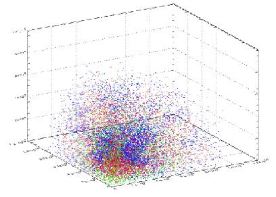
Figure 1: The positions of the Fe-rich (red), unburned (blue) and intermediate (green) tracer particles at 10 s in the c3_3d_256_10s model. Note the large amount of unburned particles in the central regions.

Initially, the tracer particles contain only ¹²C, ¹⁶O, and ²²Ne. In all the models used in the present study for $\sim$ 30 to 40 % of the particles the temperatures are sufficiently high for nucleosynthesis to transform the initial composition all the way up to iron group elements. In the remaining part, on the other hand, no or only incomplete burning occurs, depending on the temperatures and densities. As the nucleosynthesis proceeds up to 10 seconds, the final abundances we use in our nebular calculations are somewhat different from those in the c3_3d_256 model at 1.5 seconds. This is mainly a consequence of the expanding computational grid in the model followed to 10 seconds, which reduces the flame resolution. The mass of carbon in unburned particles is 0.31 M_⊙ and of oxygen 0.35 M_⊙. Including also the partially processed particles, the total mass of carbon and oxygen in the model is 0.34 and 0.42 M_⊙, respectively. The remaining particles have undergone nuclear processing, resulting in intermediate mass elements and iron peak elements. We refer to these as burned particles. The total mass of ⁵⁶Ni is in the c3_3d_256_10s model 0.28 M_⊙. This comparatively low mass may be affected by the finite resolution, as we discuss below. In Fig. 1 we show the positions of the Fe-rich (red), unburned (blue), and intermediate (green) tracer particles in the c3_3d_256_10s model.

2.3 Late time spectral modeling

The modeling of late time spectra is based on the code described in detail in Kozma & Fransson (1998a). The code was originally used to model Type II supernovae and has been applied to SN 1987A (Kozma & Fransson 1998a; Kozma & Fransson 1998b). Since then the code has been improved in a number of ways, and has also been extended to apply to Type Ia supernovae (Sollerman et al. 2004). We here therefore summarize the main features and changes of the model.

The energy input to the ejecta at these late epochs is due to decays of radioactive elements formed in the explosion. In our calculations we include decays of ⁵⁶Ni to ⁵⁶Co, and ⁵⁶Fe, as well as decays of ⁵⁷Ni and ⁴⁴Ti. We calculate the amount of gamma-ray and positron energy deposited into heating, ionization, and excitation, by solving the Boltzmann equation, as formulated by Spencer & Fano (1954). The relative fractions going into these channels depend on the composition and degree of ionization. In our model the gamma-ray and positron deposition is therefore calculated for each tracer particle separately. Our treatment of the nonthermal deposition is described in detail in Kozma & Fransson (1992).

The temperature, ionization and level populations in each tracer particle are calculated in steady state for a specific time by solving the statistical equations, together with the energy balance. We find that steady state is a good approximation up to  500 days. At later times departures from steady state become increasingly important.

The following ions are included : H I-II, He I-III, C I-III, N I-II, O I-III, Ne I-V, Na I-II, Mg I-III, Si I-III, S I-V, Ar I-V, Ca I-III, Fe I-V, Co I-V, Ni I-II. Among these the following are treated as multilevel atoms, with the number of levels within brackets: H I (20), He I (16), O I (13), Mg I (10), Si I (21), Ca II (6), Fe I (121), Fe II (191), Fe III (112), Fe IV (45), Ni I (14), Ni II (18), Co II (108), Co III (87). To calculate the cooling and line emission from the remaining ions, the level populations are calculated in steady state, using two-, five-, or six-level atoms.

Details and references for most of the atomic data used are given in Kozma & Fransson (1998a). In addition to the atomic data given in this paper, the code has been updated specifically to model Type Ia’s (Sollerman et al. 2004). In particular, higher ionization stages of especially the iron group elements have been included. The following charge transfer reactions important for the modeling of Type Ia’s have been added : Fe I + Fe II $\rightarrow$ Fe II + Fe I, Fe I + Fe III $\rightarrow$ Fe II + Fe II, and Fe I + Fe IV $\rightarrow$ Fe II + Fe III. Rate coefficients for these three reactions are from Krstic, Stancil, & Schultz (1997), as given by Liu et al. (1998).

We have improved the modeling of iron by updating the total recombination rates and including rates to individual levels for Fe I (Nahar, Bautista, Pradhan 1997), Fe II (Nahar 1997), Fe III (Nahar 1996).

Both Co II and Co III are included as multilevel atoms. For Co II, with 108 levels, A-values are from Kurucz (1988) and Quinet (1998), and the energies are from Pickering et al. (1998). For Co III, with 87 levels, all data are from Kurucz (1988). Recombination rates to Co II and Co III are unknown. To estimate recombination rates for these ions, we use the same values as for Fe II and Fe III. We set the total recombination rates to Co II and Co III equal to the total recombination rates to Fe II and Fe III, and assume that the distribution to individual levels are similar to the individual levels in Fe II and Fe III.

Also collision strengths for the Co II and Co III transitions are unknown. As a rough approximation we set the collision strengths equal to $\Omega=0.1$ for forbidden transitions, and for the allowed transitions we use Van Regemorter’s formula (van Regemorter 1962). As we show below, the contribution of Co II-III is negligible at the epochs of interest, and the lack of atomic data for these ions is therefore for this application not serious.

In all calculations presented in this paper we assume photoionization to be unimportant. As was argued in Kozma & Fransson (1998b), the reason for this is that the high energy photons responsible for the photoionization are absorbed and scattered by lines in the ejecta. Because the number of resonance transitions at these energies are extremely large multiple resonance scattering, followed by branching into the optical, will efficiently reduce the UV-field, responsible for the photoionization. In the optical range we do take fluoresence by the Ca II H and K lines explicitly into account in our calculation of the spectra. This is done by assuming that all emission within $6000\rm\leavevmode\nobreak\ km\leavevmode\nobreak\ s^{-1}$, on the blue side of the H and K lines, to be absorbed and re-emitted in the Ca II IR-triplet and the $\lambda\lambda\leavevmode\nobreak\ 7291,7324$ lines. This is the dominant mechanism for the formation of these lines (Kozma & Fransson 1998b). Other permitted lines are included, using the Sobolev approximation to treat the scattering. We do, however, not include fluoresence and scattering from line to line. Branch et al. (2005) compare spectra modeled by the synthetic spectrum code Synow, which include multiple scattering, but not any calculation of the level populations, to observations of SN 1994D at nebular phases. From this they suggest that the effects of resonance scattering are seen at $\sim$300 days in Ca II H, K and IR-triplet, and Na I. This is in agreement with the fact that these lines, as well as several Fe II lines, are optically thick also in our calculations.

3 Results

In this section we discuss the late-time spectra based on the c3_3d_256_10s model between 300 and 500 days. The reason for concentrating on these late epochs is that the optical depths in the optical and IR ranges are then small enough not to severely affect the observed spectrum. This is usually referred to as the nebular phase. Observed spectra of high signal-to-noise (S/N) only exist up to $\sim$ 350 days, and our comparison will therefore concentrate on this epoch. From this we can then put constraints on the explosion models, such as the final amount of unburned material and density structure.

We will also briefly discuss the modeling based on the b30_3d_768, b5_3d_256, and c3_3d_256 models. However, for these three models the hydrodynamics and nucleosynthesis have only been calculated for the first 1.2 – 1.5 seconds after explosion. The ejecta have for these models not yet reached homologous expansion, and the densities in these models are significantly higher than in the c3_3d_256_10s model. As we will show, the physical conditions in the ejecta, and therefore the spectrum, are sensitive to the density structure. Therefore, it is not possible to draw any firm conclusions from late time modeling based on the 1.2s and 1.5s models. They might, however, indicate the effects of different numerical resolution and initial burning conditions on the late time spectra.

Because of the importance of the density on the physical properties and the emission, we have plotted the distribution of the number densities at 300 days for the Fe-rich, intermediate mass elements, and unburned tracer particles in model c3_3d_256_10s in Fig. 2. From this we see that there is a wide distribution in densities of the Fe-rich particles from $\sim$ $3\times 10^{4}$ to $3\times 10^{6}$, with a peak at $\sim 2\times 10^{6}$ cm^-3. The densities of the unburned particles are considerably higher, with a peak around $\sim 9\times 10^{6}$ cm^-3, while the particles with intermediate mass elements are also intermediate in densities. This is a natural consequence of the energy input due to the nuclear burning, which expands mainly the regions where burning takes place.

3.1 Spectrum

In our models we calculate the ionization, temperature and level populations, and from these the emissivity from each of the 19683 tracer particles for a given position (velocity), density, and composition. From this we then construct a spectrum. The line transfer is done in the Sobolev approximation.

As all tracer particles in these explosion models are located within one octant, the properties of each tracer particle have to be mirrored in the coordinate planes in order to model the full ejecta. This simplified way of treating the geometry introduces an artificial symmetry in the line profiles. If we, for example, view the ejecta along the positive z-axis, each of the particles in the model contributes to the emission at two distinct wavelengths. For each particle in the calculated octant, four particles, at $z_{particle}>0$, contribute to the blue wing of a line, and the other four particles, at $z_{particle}<0$, contribute to the red wing of the line. This gives rise to double-peaked line profiles, which is clearly an artifact of the assumption of symmetry with respect to the coordinate planes. This effect may be reduced by, for example, viewing the ejecta from a different angle. We have tried this and, although the artificial symmetry was reduced, it was still present.

To remove the effects of the assumed geometry we have recalculated the spectra, assuming spherical symmetry for the emission. We divide the ejecta into 50 radial zones, and sum the emission from all tracer particles within each radial interval. The line profiles and spectra are then calculated from this spherically symmetric case. Note that this is only done after we have calculated the emission from each particle. The inhomogeneities of the model in terms of density and composition, as well as the radial distribution, are therefore preserved. All the spectra presented in the figures have been calculated in this way. In the future we hope to discuss the detailed line profiles, based on a full $4\pi$ model (Röpke & Hillebrandt 2005b).

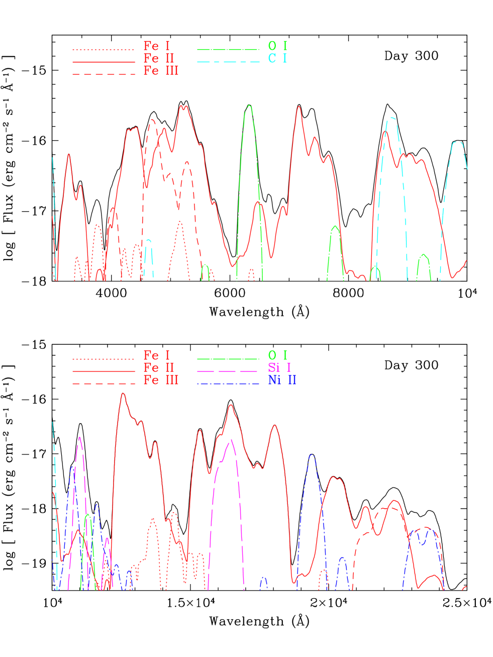
Figure 4: The dominating contributions to the model spectra from c3_3d_256_10s at 300 days. Here we show the contributions due to Fe I, Fe II, Fe III, O I, C I, Si I, and Ni II.

In Fig. 3 we show spectra for the two late epochs, 300 and 500 days past explosion, for the c3_3d_256_10s model. The spectrum at 300 days is analyzed in more detail in Fig. 4, where we show the contributions from the lines of Fe I, Fe II, Fe III, Ni II, Si I, O I, and C I.

The main difference between the spectra at the two epochs is the decrease in ionization from day 300 to day 500, as can be seen in the abundances of the iron ions. At day 500 the emission from Fe I has increased, and the emission from Fe II and III has decreased somewhat compared to the emission at 300 days. At both epochs, however, the dominant ion is Fe II.

The most interesting results of these calculations are the very strong lines from carbon and oxygen. For both epochs [C I] $\lambda\lambda\leavevmode\nobreak\ \leavevmode\nobreak\ 9824,9850$ and [O I] $\lambda\lambda\leavevmode\nobreak\ \leavevmode\nobreak\ 6300,6364$ are dominating the spectrum. At 300 days also C II] $\leavevmode\nobreak\ \lambda\leavevmode\nobreak\ \leavevmode\nobreak\ 2326$, C I $\lambda\lambda\leavevmode\nobreak\ \leavevmode\nobreak\ 2966,2968$ and [C I] $\leavevmode\nobreak\ \lambda\leavevmode\nobreak\ \leavevmode\nobreak\ 8727$ are strong, but they decrease in strength at day 500. With regard to the UV lines, it should be noted that the spectrum below $\sim 3500$ Å is very uncertain due to the effects of multiple scattering.

In the lower panel of Fig. 3 we show the IR spectrum between 1 and 2.5 $\mu$m. At these wavelengths there are no strong oxygen or carbon lines. The spectrum is dominated by Fe II, but also shows strong Si I and Ni II lines. The strongest lines are [Fe II] $1.257\mu$, $1.644\mu$ and [Si I] $1.099\mu$. The only intermediate mass element giving rise to a significant emission feature in the models is silicon. As can be seen in Fig. 3, the [Si I] $1.099\mu$ line is strong in the 300 day spectrum, while it has almost disappeared at 500 days. Cobalt does not contribute significantly to the spectra at 300 and 500 days, and the strength of the cobalt lines decreases with time. At 300 days only $\sim 7\%$ of the radioactive cobalt remains. Uncertainties in especially the cobalt collisional excitation and recombination data are therefore of minor importance. The strongest cobalt line in the models is [Co II] $1.019\mu$.

While most line features in both the optical and IR are severely blended, the IR lines are the ones least affected. For studies of line profiles these are therefore the most suitable. In particular the Ni II line from stable ⁵⁸Ni at $1.940\mu$ is from this point of view especially interesting.

In Fig. 5 we compare a model spectrum at 350 days to observations of SN 1998bu on day 398, SN 2000cx on day 378, and SN 2001el on day 336 after explosion. We have renormalized the flux of the three spectra to 350 days, using a decline rate of 0.0138 mags per day in the V band (Sollerman et al. 2004). We have also scaled the observed spectra to a common distance of 10 Mpc.

The spectrum of SN 1998bu, taken from Spyromilio et al. (2004), was obtained at 398 days after explosion. This is one of the best S/N spectra available at this epoch, and one of the few covering the region above 8000 Å. A problem is, however, that the spectrum is contaminated by a light echo (Cappellaro et al. 2001), which especially in the blue gives a substantial contribution to the flux. We have removed this as discussed in Spyromilio et al. (2004). For the reddening of SN 1998bu we adopt $E_{\rm B-V}=0.30$ and a distance of 11 Mpc (Suntzeff et al. 1999). SN 1998bu has a normal luminosity and decline rate.

SN 2000cx was observed using VLT/FORS 360 days past maximum light. These observations were performed with the 300V grism, an order-sorting filter GG375 and a $1\hbox{$.\!\!^{\prime\prime}$}3$ wide slit. The data were reduced in a standard way, including flux-calibration using spectrophotmetric standard stars, as outlined by Sollerman et al. (2004). For the smoothed spectrum of SN 2000cx shown in Fig. 5 we use a reddening $E_{\rm B-V}=0.08$ (Schlegel et al. 1998) and a distance of 33 Mpc (Candia et al. 2003). SN 2000cx was a rather peculiar SN Ia around maximum light, peculiarities including an unusual light-curve and an unusual color evolution (Li et al. 2001). However, as shown in Sollerman et al. (2004), at later phases the light curve for this supernova actually behaved quite normally. In Fig. 5 we also compare the late spectrum from SN 2000cx to the two other SN Ia and we find that, at these epochs, the three spectra are quite similar.

The observations of SN 2001el were obtained with the same instrumental set-up as for SN 2000cx at an epoch of 318 days past maximum. For the reddening we adopt $E_{\rm B-V}=0.25$ and a distance of 17.9 Mpc (Krisciunas et al. 2003). SN 2001el was a rather normal SN Ia as far as its luminosity and decline rate are concerned (Krisciunas et al. 2003), but it was the first “normal” SN Ia that showed strong intrinsic polarization and a high velocity detached Ca II IR triplet, interpreted as a clumpy shell (Kasen et al. 2003).

The first thing to note from the comparison of the model with the observed spectra is the general similarity of most of the strong features in the spectrum. In particular, this applies to the Fe II-III features, which are all seen, albeit with somewhat different relative fluxes (see below). The absolute level of the model spectrum is lower than the observed spectra, which is explained by the low ⁵⁶Ni mass in the c3_3d_256_10s model. Considering the limitations of the explosion models, we find the general agreement of models and observations very promising. With this background we now discuss the shortcomings of this model.

Comparing the synthetic spectrum with the observed, it is obvious that the dominant lines in the modeled spectrum, [O I] $\lambda\lambda\leavevmode\nobreak\ \leavevmode\nobreak\ 6300,6364$ and [C I] $\leavevmode\nobreak\ \lambda\leavevmode\nobreak\ \leavevmode\nobreak\ 8727$, are not present in the observations. This is particularly obvious for the [O I] line, where the peak is close to a ’valley’ between two emission features in the observed spectra. The [C I] region is only covered by the SN 1998bu and SN 2000cx spectra. There is in the SN 1998bu spectrum indeed a feature close to the [C I] line, but a closer inspection shows that this is centered at $\sim 8600$ Å, rather than at 8727 Å. The origin of this is therefore most likely Fe II $\leavevmode\nobreak\ \lambda\leavevmode\nobreak\ 8621$, rather than [C I]. The strong [C I] and [O I] lines are the most serious discrepancies of the models, and show that these explosion models have too large masses of these elements in the central regions of the explosion model. We discuss this further in section 4.

A less serious discrepancy is that the c3_3d_256_10s model is not able to satisfactorily reproduce the characteristic three-bump feature between 4500 Å  and 5500 Å. In particular, the observed strong bump at $\sim$ 4700 Å, which is mainly due to Fe III (Fig. 4), is too weak in the model, as can be seen in Fig. 5. This indicates that the model has a too low degree of ionization.

Another slight discrepancy is the feature seen in the observations between 5700 and 6200 Å, but which is absent in the model. This region is in the model dominated by Fe II emission. In addition Si I, Fe I, Fe IV, Co II, and Ni II have transitions at these wavelengths.

In Fig. 6 we compare the modeled IR spectrum at 350 days to observations of SN 1998bu at 344 days from Spyromilio et al. (2004). We find that the model in this wavelength region is able to reproduce most of the features seen in the observations. In particular, the relative strengths of the different Fe II lines agree very nicely with the observations. There is an indication that the [Si I] $1.099\mu$ line is also present. Unfortunately, the observed spectrum only covers half of the line.

The densities in the other three explosion models, which were only calculated up to 1.2 – 1.5 seconds, are significantly higher than for the 10 second model, if scaled to the same epoch. If run to the homologous stage they would, however, most likely end up with a lower density. In particular, the b30_3d_768 model has the highest kinetic energy and may therefore end up as the lowest density model. Nevertheless, these models demonstrate that higher densities result in lower temperatures and lower degrees of ionization. Therefore, for these models the Fe III bump is completely absent.

In the near-IR, the low degree of ionization in these models result in a strong [Fe I] $1.443\mu$ line, which is very weak in the c3_3d_256_10s model. The same is true for the [Si I] $1.099\mu$ line. The fluxes of the O I and C I lines are in these models considerably stronger. This demonstrates the importance of the density structure of the explosion model to the late time spectra. The fact that these models were not calculated to the homologous stage therefore makes any conclusions on these models very uncertain.

To analyze the differences between the observations and model, and because the spectrum reflects the temperature and ionization of the ejecta, we now discuss in more detail how these quantities vary in the models.

3.2 Temperatures

Because of the large range in density and composition of the ejecta, the temperature and ionization will be highly inhomogeneous, depending on the composition, density, and to a certain degree the geometrical position of the tracer particle. This is one of the most important differences between 1D and 3D models.

At 300 days (500 days) the temperatures in the unburned C/O/Ne particles, vary from $\sim$2600 K to $\sim$8500 K (600 to 6000 K), with a characteristic temperature of $\sim$ 5000 K (3000 K). The highest temperatures are found at the largest radii. The reason is that the particles closest to the center, having the highest density, also undergo the fastest cooling (Axelrod 1980). Away from the center the densities decrease, and the temperatures increase.

To further illustrate the highly inhomogeneous nature of the ejecta conditions, we show in Fig. 7 the temperatures of the Fe-rich mass elements at 300 and 500 days, where we have plotted the density and temperature for each of the Fe-rich mass elements. These particles have densities in the range $\sim 3\times 10^{4}$ cm^-3 to $\sim 3\times 10^{6}$ cm^-3 at 300 days (Fig. 2). At 300 days most of the mass elements are found in two temperature regions (along the two boundaries seen in Fig. 7), at $\sim$ 2000 K, and $4000-5000$ K, respectively.

For a given density the variation in temperature, as seen in Fig. 7, is due to different ⁵⁶Ni-abundances in the mass elements. The temperatures of the tracer particles show two boundaries in Fig. 7, where most of the particles are found. These contain the most ⁵⁶Ni-poor (lowest temperatures) and most ⁵⁶Ni-rich (highest temperatures) mass elements, respectively. For a given ⁵⁶Ni fraction, the temperature increases with decreasing densities. The particles at the low-temperature boundary are composed of stable iron (mainly ⁵⁴Fe) with a mass fraction of $\sim 0.7$, and stable nickel (mainly ⁵⁸Ni) with a mass fraction of $\sim 0.3$. In these particles only $\sim 5\times 10^{-4}$ of the mass is radioactive ⁵⁶Ni. At the high-temperature boundary, on the other hand, the mass fraction of ⁵⁶Ni is $\sim 0.9$.

The nucleosynthesis taking place within a tracer particle is determined mainly by the peak temperature and density of the particle. If the temperature is sufficiently high, T$\!\!\!\phantom{\geq}\smash{\buildrel\over{\lower 2.67502pt\hbox{$\buildrel\lower 2.14001pt\hbox{$\displaystyle>$}\over{\sim}$}}}\,\,6\times 10^{9}$ K (Travaglio et al. 2004), nuclear statistical equilibrium (NSE) is reached, resulting in a composition dominated by iron-peak elements. The final composition of a particle reaching NSE depends on both on the temperature and density and also on the neutron excess ($\eta$), which is detemined by the amount of electron capture taking place. The higher the neutron excess the more neutron rich isotopes such as ⁵⁸Ni and ⁵⁴Fe form.

At 500 days the temperatures have decreased significantly, as seen in Fig. 7. The temperatures are now peaked at $\sim$ 500 K and $\sim$ 3000 K. For the ⁵⁶Ni-rich particles the density and temperature still correlate, so that the temperatures in the mass elements with lower densities are higher than in the mass elements of higher densities.

For the ⁵⁶Ni-poor particles on the other hand, the temperatures of the particles are more or less constant, independent of density. The reason is that at these low temperatures cooling by far-IR Fe II fine structure lines is becoming important. For the high density, low temperature regions, the ionization is lower (see the right panels in Fig. 7), resulting in a higher abundance of Fe I than of Fe II, and a less efficient cooling. Therefore, for these particles the cooling is determined both by the ratio of Fe I/Fe II and density.

The spread in temperatures for the Fe-rich particles in the b30_3d_768, b5_3d_256, and the c3_3d_256 models are smaller than for the c3_3d_256_10s model. This depends mainly on the differences in densities. The higher the density is, the smaller the spread in temperature will be.

Also for particles not burned all the way to NSE, rich in intermediate mass elements, we find that particles with similar compositions gather along certain boundaries. The temperatures for some of these particles are even higher than for the Fe-rich particles rich in ⁵⁶Ni, due to the less efficient cooling in these particles.

3.3 Ionization

In the right panels of Fig. 7 we show the electron fraction as function of density within each Fe-rich mass element at 300 and 500 days for the c3_3d_256_10s model. The electron fraction, x_e, is here defined as the ratio of the number density of free electrons, n_e, to the total number density of neutral atoms and ions, n, i.e. x_e = n_e/n. At 500 days the electron fraction varies from $\sim$ 0.4 to $\!\!\!\phantom{\geq}\smash{\buildrel\over{\lower 2.67502pt\hbox{$\buildrel\lower 2.14001pt\hbox{$\displaystyle>$}\over{\sim}$}}}\,\,$ 3, depending on density. The lower boundary of the electron fractions at 300 days is a factor of $\sim 1.5$ higher. The same boundaries as seen for the temperature are present for the electron fraction in Fig. 7. This means that the upper boundaries in the plots include the most ⁵⁶Ni-rich particles, while the mass elements along the lower boundary contains the least ⁵⁶Ni. As is clearly seen in these figures, a decrease in density results in an increase in electron fraction (for a given ⁵⁶Ni mass) due to reduced recombination rates.

As expected, the degree of ionization decreases as the energy input decreases. At both epochs Fe II is the dominant ion. However, at 500 days the Fe I abundance is $\!\!\!\phantom{\geq}\smash{\buildrel\over{\lower 2.67502pt\hbox{$\buildrel\lower 2.14001pt\hbox{$\displaystyle>$}\over{\sim}$}}}\,\,\ 0.1$, in the high density regions. Conversely, Fe III becomes increasingly important as energy input increases.

Similar to the temperature, the spread in electron fraction for the Fe-rich particles in the b30_3d_768, b5_3d_256, and the c3_3d_256 models are smaller than for the c3_3d_256_10s model. The higher densities in these models result in a lower degree of ionization.

For all models we have assumed that the positrons deposit their energy locally in the mass elements containing the newly synthesized nickel. If we instead assume non-local deposition of the positrons (Milne et al. 1999, 2001), the Fe III abundance would decrease, making the ionization problem even worse. On the other hand, the degree of ionization in the unburned regions would increase somewhat, reducing the strength of the O I and C I lines. This effect is, however, probably small.

4 Discussion

Models of early Type Ia supernova spectra, based on 3D hydrodynamical models, have been developed by Thomas et al. (2002), and Thomas (2003). They have used a modified version of the spectrum code SYNOW to include effects of non-spherical symmetric geometries. In particular, Thomas et al. have studied the effects of non-spherical inhomogeneities on the line profiles. This has in contrast to this paper mainly been in the context of early stages, and at high velocities. In Thomas et al. (2004) the high velocity Ca II features seen in SN 2000cx near maximum light are modeled, based on 3D ejecta models. They find that 3D models are required to explain the Ca II features, and they also estimate the mass of the high velocity ejecta.

Our conclusions with regard to unburned carbon and oxygen in the ejecta are complementary to previous studies using early epoch spectra. Observations in the near infrared region (Marion et al. 2003) of twelve supernovae near maximum light, show no sign of unburned carbon at velocities above $\sim 3000\rm\leavevmode\nobreak\ km\leavevmode\nobreak\ s^{-1}$. Based on these observations they put a limit to the amount of unburned matter to $\!\!\!\phantom{\leq}\smash{\buildrel\over{\lower 2.67502pt\hbox{$\buildrel\lower 2.14001pt\hbox{$\displaystyle<$}\over{\sim}$}}}\,\,$ 10% of the progenitor mass.

By comparing observed spectra of SN 2002bo to 1D synthetic spectra at different times, both around maximum light and in the nebular phase, Stehle et al. (2004) derive the abundance distribution of the supernova ejecta. They find a ⁵⁶Ni mass of 0.52 M_⊙ and evidence for intermediate mass elements at high velocities. They find no sign of carbon lines at any velocities, and inferred an upper limit of the total mass of carbon to $1.6\times 10^{-3}$ M_⊙. The corresponding mass for oxygen was 0.11 M_⊙ where it is most dominant at high velocities, and no oxygen was observed below $6000\rm\leavevmode\nobreak\ km\leavevmode\nobreak\ s^{-1}$.

Further, in order to examine the mixing of unburned material to low velocities, as seen in 3D deflagration models, Baron et al. (2003) modified the composition of the 1D, deflagration model W7 (Nomoto et al. 1984; Thielemann et al. 1986) by introducing unburned material into the central regions. They modeled the spectra from 3000 – 8000 Å at 15-25 days past maximum, and concluded that it was, from their models, not possible to rule out the presence of unburned material at low velocities. As a consequence of this, they pointed out the importance of modeling of late time nebular spectra, based on actual 3D hydrodynamical models, in order to resolve these questions. This is demonstrated by our calculations.

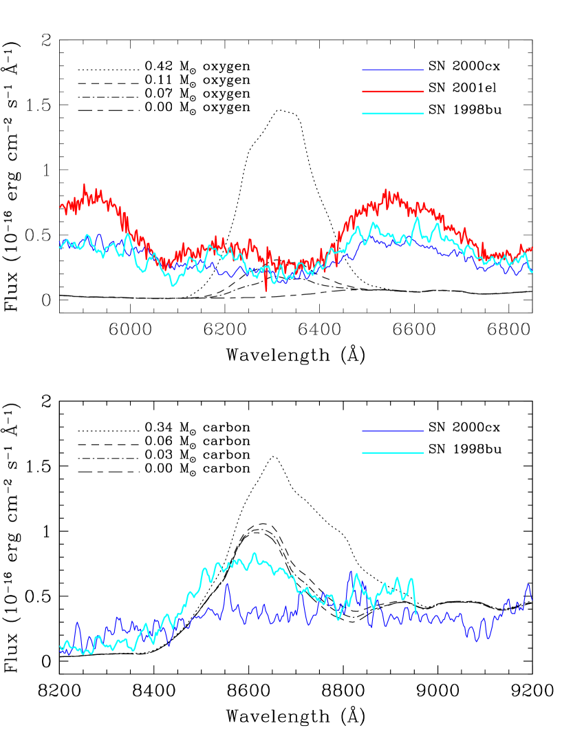
Figure 8: The region around the [O I] $\lambda\lambda\leavevmode\nobreak\ \leavevmode\nobreak\ 6300,6364$ and [C I] $\leavevmode\nobreak\ \lambda\leavevmode\nobreak\ \leavevmode\nobreak\ 8727$ lines based on the c3_3d_256_10s model at 350 days together with observed spectra for SN 2000cx, SN 2001el and SN 1998bu. The original model, containing 0.42 M_⊙ of oxygen and 0.34 M_⊙ of carbon (dotted curves), is compared to models where the masses of oxygen and carbon have been artificially reduced. The dot-dashed curve includes only the partially burned regions, with $\sim 0.03$ M_⊙ carbon and $\sim 0.07$ M_⊙ oxygen, while the dashed curve also has additional 0.03 M_⊙ carbon and 0.04 M_⊙ oxygen from unburned material. The remaining feature in the oxygen and carbon free model at $\sim 8600$ Å  is due to Fe II.

The synthetic nebular spectra presented in this paper show strong carbon and oxygen lines in contradiction to our observations. This fact demonstrates that the amount of unburned material in the center of these explosion models is too large. In order to estimate an upper limit to the mass of unburned matter in the central region allowed from the nebular spectra, we have recalculated the spectra from the c3_3d_256_10s model with varying amounts of unburned matter. The results are shown in Fig. 8, where we show the spectra in the wavelength regions containing the [O I] $\lambda\lambda\leavevmode\nobreak\ \leavevmode\nobreak\ 6300,6364$ and [C I] $\leavevmode\nobreak\ \lambda\leavevmode\nobreak\ 8727$ lines, together with observations of SN 1998bu, SN 2000cx, and SN 2001el. The absolute flux calibration of the spectra of SNe 1998bu and 2000cx is performed by comparison to contemporary broad band photometry. For SN 2001el we use a late time magnitude based on the assumption that this supernova has the same time-evolution ($\Delta$ m${}^{\rm 350}_{\rm V}$) as the well observed SN 1996X. We integrate the spectra under the V band filter function and scale it to match the extrapolated late V band magnitude. Finally, the spectra are corrected for Galactic extinction, transferred to a common distance and scaled to a common epoch.

The dotted curve in Fig. 8 shows the original model. The model contains in total 0.42 M_⊙ of oxygen and 0.34 M_⊙ of carbon, residing both in the unburned particles and in the partially burned particles. Note that the observed spectra are calibrated on an absolute scale. We can therefore directly compare the fluxes in the O I and C I lines with the observations, and not only relative to the ’continuum’.

As an extreme we have artificially removed all carbon and oxygen emission in one model, shown as the lowest short-long dashed line in Fig. 8. We also show two models where we have varied the number of unburned particles. In the first we removed all unburned particles, including only the carbon and oxygen residing in the partially burned particles (0.07 M_⊙ of oxygen and 0.03 M_⊙ of carbon). In the second we reduced the number of unburned particles by a factor of 10, resulting in oxygen and carbon masses of 0.11 M_⊙ and 0.06 M_⊙, respectively. From this figure it is seen that the original model is in clear disagreement with the observations for both the C I and O I lines. The model with only the carbon and oxygen in the partially burned particles is just compatible with the observations. As an upper limit to the unburned mass we estimate this to be close to the 0.03 M_⊙ of carbon and 0.04 M_⊙ of oxygen in the dashed line model in Fig. 8. This is in addition to the carbon and oxygen in the partially burned gas. We do stress that these limits only apply to the low velocity gas in the core.

Although we do not find any signs of oxygen in our observations there are early claims in the literature of detection of [O I] $\lambda\lambda\leavevmode\nobreak\ \leavevmode\nobreak\ 6300,6364$ in SN 1937C (Minkowski, 1939). This has, however, not been confirmed by modern observations.

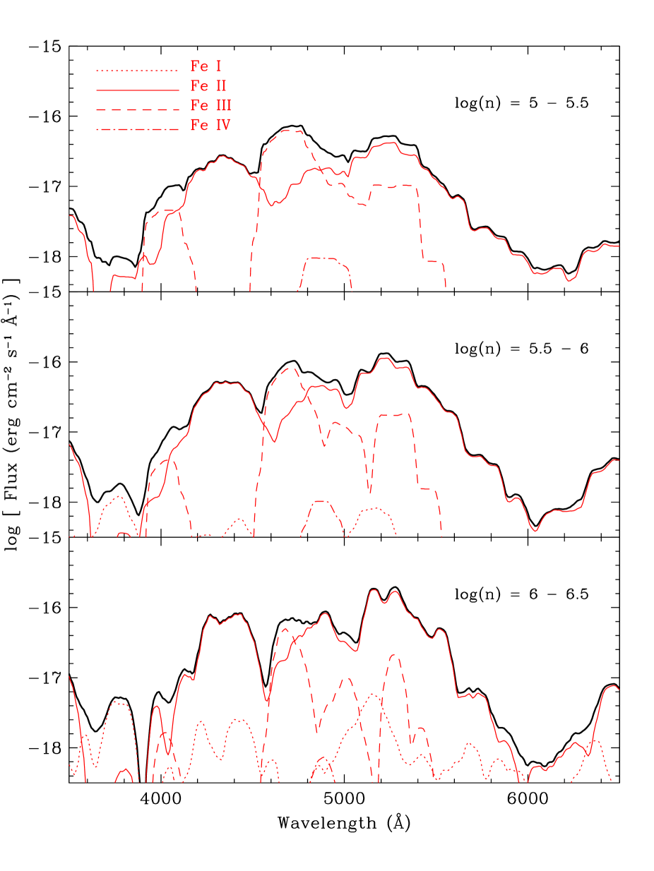
Figure 9: Spectra based on the c3_3d_256_10s model at 300 days. The upper panel shows the spectrum from the Fe-rich particles in the density range $10^{5}-3\times 10^{5}$ cm^-3, the middle spectrum from those in the range $3\times 10^{5}-10^{6}$ cm^-3 and the lower panel the spectrum from those in the range $10^{6}-3\times 10^{6}$ cm^-3. The thick, solid line gives the total flux from these density ranges.

In the wavelength range 4500 – 5500 Å the observations show three characteristic bumps (Fig. 5). These can all be seen in the model, and are explained as a mixture of Fe II and Fe III emission. The relative strengths of the Fe II and Fe III features are sensitive to the densities in the emitting gas. In Fig. 9 we show the contributions from the different ionization stages of iron to this wavelength region for particles of different density ranges. In the upper panel we show the contribution from the Fe-rich tracer particles in the range $(1-3)\times 10^{5}$ cm^-3, and in the two lower panels for the density ranges $(3-10)\times 10^{5}$ cm^-3 and $(1-3)\times 10^{6}$ cm^-3. The contributions to the total flux in this wavelength region from the above density ranges are 17 %, 34 % and 49 %, respectively.

Fig. 9 clearly shows the effects of varying the density. Especially the strength of the Fe III feature around 4600 – 4800 Å is sensitive to the density of the emitting gas. An increase in density reduces the degree of ionization, due to increased recombination rates, and consequently the Fe II abundance increases relative to Fe III. In the c3_3d_256_10s model both the Fe II peaks at $\sim$ 4300 Å and at $\sim$ 5200 Å , as well as the Fe III peak, are clearly seen in Fig. 5. Compared to the observed spectra, the relative fluxes of the two Fe II peaks are well reproduced. The ratio of the flux in the Fe II and Fe III peaks is, however, a factor of $\sim 2-3$ too large compared to the observations. A decrease in the density compared to the c3_3d_256_10s model is therefore indicated from these observations. Also the too strong Fe II complex at 7000 – 8000 Å, and the blend of Fe II and C I at 8500 – 9500 Å  indicate a too low ionization. In addition, the large dip in the model spectrum at $\sim$ 6000 Å would be reduced by a lower density.

In the other three non-homologous models the densities are even higher, and Fe II is totally dominating the spectrum in this wavelength region. From this we see the importance of following the hydrodynamical calculations until homologous expansion is reached.

In addition to decreasing the densities, an alternative way to increase the ionization is to increase the amount of ⁵⁶Ni formed in the explosion. The amount of ⁵⁶Ni in the c3_3d_256_10s model is only 0.28 M_⊙. The reason for this low value (which is not typical for pure deflagration models) was discussed in Sec. 2.1. In Table 1 the masses of ⁵⁶Ni are given for all the models on which the present paper is based. In the model with the highest resolution (model b30_3d_768) also the largest mass of ⁵⁶Ni is formed, i.e. 0.42 M_⊙. These values are still at the low end of what is derived from observations. Contardo et al. (2000) estimate ⁵⁶Ni-masses from observed UBVRI light curves for a number of type Ia supernovae, and find M(⁵⁶Ni) = 0.40 – 1.1 M_⊙, except for SN 1991bg with M(⁵⁶Ni) = 0.11 M_⊙. For comparison, the popular W7 model has M(⁵⁶Ni) = 0.60 M_⊙. A higher ⁵⁶Ni abundance increases the ionization, and thus would improve the agreement with the observed spectra shown in Fig. 5.

To test this hypothesis we have made one-dimensional spectrum calculations based on the W7 model, which will be discussed in more detail in Kozma & Fransson (2005). We find that at 300 days this model reproduces the observations quite well. In particular, the [Fe III] features are now better reproduced. At 300 days the densities in the Fe-rich zones in the W7 model vary from $1.2\times 10^{5}$ cm^-3 to $1.5\times 10^{6}$ cm^-3. This range corresponds to the upper two spectra in Fig. 9. From this we conclude that the reason why the W7 model reproduces the observed spectra better than the c3_3d_256_10s model is the combination of a lower mean density and a higher ⁵⁶Ni mass.

If we compare the synthetic spectra based on the non-homologous c3_3d_256 and b30_3d_768 models at 300 and 500 days (not shown here), we find that both models show too strong O I and C I lines. The ¹²C and ¹⁶O masses for the different models are given in Table 1. While there is a considerable difference in these masses depending on the resolution and initiation of the burning, this is not enough to solve the problem with the strong O I and C I features. This could be due to the fact that model b30_3d_768 was not evolved far enough in time. But it could also reflect a deeper problem of the models.

There are several assumptions and uncertainties in the 3D hydro calculations that might affect the still existing differences between the computed late time spectra and our observations. First of all, low-resolution models such as the c3_3d_256_10s model have been computed with the aim to analyze differences in the model predictions resulting from different physical parameters, for instance the C-to-O ratio (Röpke & Hillebrandt 2004), the metallicity, and the ignition density. They are not meant to give realistic models of the explosion. Models with higher resolution (such as model b30_3d_768) are more realistic, and for given initial conditions they seem to be almost “converged” as far as global properties are concerned, i.e. the Ni-mass and the explosion energy. But these models have not yet been evolved far enough to make safe predictions for the density, the temperature, and the element distribution in velocity space. However, we can predict from model b30_3d_768 that in models with higher numerical resolution the amount of unburned material at low velocities will be less and more ⁵⁶Ni will be formed.

Additional uncertainties result from the (unknown) ignition conditions, the still rather ad-hoc sub-grid scale model for the burning velocity (Schmidt et al. 2005), the poorly known physics of thermonuclear burning in the distributed regime at low densities (Röpke & Hillebrandt 2005a), or the need to perform full-star computations in order to avoid artificial symmetries (Röpke & Hillebrandt 2005b). Whether or not all these necessary modifications of the models will reduce the amount of unburned carbon and oxygen to the low values indicated by the observed nebular spectra is an open question, and will be addressed in future papers.

Another way to avoid the low velocity carbon and oxygen, as well as increasing the ⁵⁶Ni-mass, could be to invoke a delayed detonation (Khokhlov 1991; Yamaoka et al. 1992; Niemeyer & Woosley 1997). Light curve modeling by Höflich & Khokhlov (1996), based on 1D simulations, has shown that delayed detonations give good fits to the light curves and early spectra, provided the transition density from the deflagration to the detonation phase is properly adjusted, introducing a new free parameter. Recently Gamezo et al. (2004a, 2004b) found in a 3D model that a transition from deflagration to detonation can remove efficiently low velocity carbon and oxygen. In addition, the mass of ⁵⁶Ni increased considerably.

Plewa et al. (2004) present a gravitationally confined detonation mechanism in which a single rising deflagration bubble triggers a detonation near the stellar surface. These models are thought to result in mildely asymmetric explosions, and with energetics and chemical composition similar to those of the delayed detonation models.

It is, however, in our view premature to draw any strong conclusions of a preferred explosion mechanism in either direction. In particular, it is not at all clear what kind of physics might cause a transition to a detonation. On the contrary, all investigations carried out so far seem to rule out the mechanisms responsible for deflagration-to-detonation transitions in laboratory combustion for SNe Ia (Niemeyer 1999; Lisewski et al. 2000; Röpke et al. 2004a, 2004b; Bell et al. 2004). Moreover, it is unclear even whether or not a detonation ignited in one pocket of unburned C-O fuel can incinerate the rest of the already fast expanding star. Because the detonation front in a SN Ia is weak and propagates with sonic velocity pressure waves may not be able to penetrate through regions consisting of burned material. It is quite possible that numerical diffusion has caused the almost complete burning found in the simulation of Gamezo et al. (2004a, 2004b) (Niemeyer, Livne, private communication).

5 Summary

Our main aim in this paper is to show the potential of testing multidimensional explosion models by detailed modeling of the emission later than $\sim$ 100 days after the explosion. To do this we have calculated late time spectra based on 3D hydrodynamical and nucleosynthesis simulations. We have mainly studied one model which has been calculated to the homologous stage, c3_3d_256_10s, at two different epochs, 300 and 500 days, but also investigated three other less evolved models, to get an idea of how the still limited numerical resolution of today’s 3D models and the initiation of burning might affect the conclusions.

Our results can be summarized in the following points:

• The observed features in both the optical and IR spectra, dominated by Fe II-III emission, are qualitatively well reproduced, given the minimum of free parameters in the explosion models.
  

• The models, however, as they stand predict strong carbon and oxygen lines, in particular [C I] $\leavevmode\nobreak\ \lambda\leavevmode\nobreak\ \leavevmode\nobreak\ 8727$, [C I] $\lambda\lambda\leavevmode\nobreak\ \leavevmode\nobreak\ 9824,9850$ and [O I] $\lambda\lambda\leavevmode\nobreak\ \leavevmode\nobreak\ 6300,6364$, at both epochs. The strong [O I] in the model predictions is clearly in conflict with the observations. As far as [C I] is concerned the conclusions are based only on a few spectra. Unfortunately there exist only a few published SNe Ia late spectra which extend to the red beyond 8000 Å. Nonetheless, from the comparison between the models and observations we think we can set an upper limit of the unburned mass inside of $\sim 10^{4}\leavevmode\nobreak\ \rm\leavevmode\nobreak\ km\leavevmode\nobreak\ s^{-1}$ of $\sim$ 0.07 M_⊙ for the published cases. We emphasize that this only applies to material lower than this velocity. At higher velocities late epoch spectra are less sensitive because of the low gamma-ray deposition rate there.
  

• In the models the temperature and ionization in the different mass elements vary strongly, depending mainly on the composition and density of the mass elements. From 300 days to 500 days the temperatures decrease significantly. At 500 days a fraction of the Fe-rich mass elements starts to undergo the IR-catastrophe, and their temperatures have dropped to $\sim 500$ K. At the same epoch there are regions with temperatures $\!\!\!\phantom{\geq}\smash{\buildrel\over{\lower 2.67502pt\hbox{$\buildrel\lower 2.14001pt\hbox{$\displaystyle>$}\over{\sim}$}}}\,\,5000$ K. This illustrates the need of detailed modeling based on 3D explosions, and shows that 1D models for the spectra are a poor approximation for pure deflagration models.
  

• The ionization in the models used in this study is somewhat too low in comparison to the supernovae for which late spectra exist. This can be seen from the Fe II-III features in the wavelength interval 4500 – 5500 Å. By increasing the mass of ⁵⁶Ni and/or reducing the densities, we would get a higher ionization and a better agreement with observations. Model b30_3d_768, if evolved into homologous expansion, would give us lower densities as requested, indicating the need for such elaborate (and expensive) models. Again, the Fe II-III features in the late nebular spectra provide excellent measures to test the explosion models based on the observations of individual supernovae.
  

To conclude, we have demonstrated that modeling of late spectra can put strong constraints on the hydrodynamics and nucleosynthesis in the explosion. In the future we intend to explore more realistic explosion models, as well as a more accurate scheme for radiative transfer in the optical range. The calculations presented here should in this context be seen as a first step.

Acknowledgements. We are grateful to Ken Nomoto for helpful discussions, to Sultana Nahar for supplying atomic data in advance of publication, and to David Branch for valuable comments and suggestions. Financial support for this work was provided to the Stockholm group by the Swedish National Space Board and Swedish Research Council. This work was supported in part by the European Research Training Network ”The Physics of type Ia Supernova Explosions” under contract HPRN-CT-2002-00303.

Model	Mode of ignition	Grid size	Time	M(56Ni)	M(unburned O)	M(unburned C)	Kinetic energy
			(s)	(M⊙)	(M⊙)	(M⊙)	(ergs)
b30_3d_768	30 bubbles	$768^{3}$	1.2	0.42	0.26	0.28	$6.7\times 10^{50}$
b5_3d_256	5 bubbles	$256^{3}$	1.5	0.33	0.29	0.24	$5.1\times 10^{50}$
c3_3d_256	central	$256^{3}$	1.5	0.31	0.34	0.35	$4.4\times 10^{50}$
c3_3d_256_10s	central	$256^{3}$	10	0.28	0.35	0.31	$\sim 4.4\times 10^{50}$

Table 1: The explosion models studied in this paper from Travaglio et al. (2004), and from Röpke (2005). The time in this table is the time for which the hydrodynamics and nucleosynthesis has been calculated.

Figure 2: The distribution of number densities for the tracer particles in the c3_3d_256_10s model at 300 days.

Figure 3: Model spectra at 300 days (thick lines) and 500 days (thin lines) for the c3_3d_256_10s model. The distance is assumed to be 10 Mpc.

Figure 5: Model spectrum at 350 days, for the c3_3d_256_10s model compared to observations of SN 1998bu from day 398, SN 2000cx from day 378, and of SN 2001el from 336 days after explosion. For clarity the observed spectra have been shifted relative to each other, the SN 1998bu spectrum by $-$4 dex, the SN 2000cx spectrum by $-$7 dex, and the SN 2001el spectrum by $-$10 dex. The observed spectra have been smoothed, dereddened, normalized to 350 days, and rescaled to a common distance of 10 Mpc as discussed in section 3.1.

Figure 6: Model IR spectrum at 350 days, for the c3_3d_256_10s model compared to observations of SN 1998bu from day 344 (Spyromilio et al. 2004). For clarity the observed spectrum has been shifted by $-$4 dex. The observations have been cleaned and heavily smoothed, using a Savitzky-Golay polynomial smoothing filter with a width of 50 wavelengthbins, corresponding to $\sim 4500\rm\leavevmode\nobreak\ km\leavevmode\nobreak\ s^{-1}$.

Figure 7: The crosses mark density and temperature (left hand panels) and density and electron fraction (right hand panels) for each of the Fe-rich mass elements the c3_3d_256_10s model at 300 (upper panel) and 500 days (lower panel).

References

- (1) Axelrod, T. S. 1980, Ph.D. thesis, Univ. California, Santa Cruz
- (2) Baron, E., Lentz, E. J., & Hauschildt, P. H. 2003, ApJ, 588, L29
- Bell et al. (2004) Bell, J. B., Day M. S., Rendleman, C. A., Woosley, S. E., & Zingale M. 2004, ApJ, 608, 883
- Branch et al. (2005) Branch, D., Baron, E., Hall, N., Melakayil, M., & Parrent, J. 2005, PASP in press, astro-ph/0503165
- Candia et al. (2003) Candia, P., Krisciunas, K., Suntzeff, N. B., et al. 2003, PASP, 115, 277
- Cappellaro et al. (2001) Cappellaro, E., et al. 2001, ApJ, 549, L215
- (7) Contardo, G., Leibundgut, B., & Vacca, W.D. 2000, A&A, 359, 876
- (8) Gamezo, V. N., Khokhlov, A. M., Oran, E. S., Ctchelkanova, A. Y., & Rosenberg, R. O. 2003, Science, 299, 77
- Gamezo, Khokhlov, & Oran (2004) Gamezo, V. N., Khokhlov, A. M., & Oran, E. S. 2004a, Physical Review Letters, 92, 21
- Gamezo, Khokhlov, & Oran (2004) Gamezo, V. N., Khokhlov, A. M., & Oran, E. S. 2004b, submitted to ApJ, astro-ph/0409598
- Garcia-Senz and Bravo (2005) Garcia-Senz, D., & Bravo, E. 2005, A&A 430, 585
- (12) Garcia-Senz, D., & Woosley, S. E. 1995, ApJ 454, 895
- Hoeflich & Khokhlov (1996) Höflich, P. & Khokhlov, A. 1996, ApJ, 457, 500
- Höflich & Stein (2002) Höflich, P. & Stein, J. 2002, ApJ, 568, 779
- (15) Iwamoto, K., Brachwitz, F., Nomoto, K. I., et al. 1999, ApJS, 125, 439
- Khokhlov (1991) Khokhlov, A. M. 1991, A&A, 245, 114
- (17) Kasen, D., Nugent, P., Wang, L., Howell, D. A., Wheeler, J. C., Höflich, P., Baade, D., Baron, E., & Hauschildt, P. H. 2003, ApJ 593, 788
- (18) Kozma, C. & Fransson, C. 1992, ApJ, 390, 602
- (19) Kozma, C. & Fransson, C. 1998a, ApJ, 496, 946
- (20) Kozma, C. & Fransson, C. 1998b, ApJ, 497, 431
- Kozma & Fransson (2005) Kozma, C. & Fransson, C. 2005, in preparation
- (22) Krisciunas, K., Suntzeff, N. B., Candida, P., et al. 2003, AJ, 125, 166
- (23) Kurucz, R. L. 1988, Trans. IAU, XXB, ed. M. McNally, Dordrecht: Kluwer, p. 168.
- (24) Langanke, K., & Martinez-Pinedo, G. 2000, Nucl. Phys. A, 673, 481
- (25) Li, W., Filippenko, A. V., Gates, E., et al. 2001, PASP, 113, 1178
- Lisewski, Hillebrandt, & Woosley (2000) Lisewski, A. M., Hillebrandt, W., & Woosley, S. E. 2000, ApJ, 538, 831
- (27) Liu, W., Jeffery, D. J., & Schultz D. R. 1998, ApJ, 494, 812
- (28) Marion, G. H, Höflich, P., Vacca, W. D., & Wheeler, J. C. 2003, ApJ, 591, 316
- (29) Martinez-Pinedo, G., Langanke, K., & Dean, D. J. 2000, ApJS, 126, 493
- (30) Milne, P. A., The, L.-S., Leising, M. D. 1999, ApJS, 124, 503
- (31) Milne, P. A., The, L.-S., Leising, M. D. 2001, ApJ, 559, 1019
- (32) Minkowski, R. 1939, ApJ, 89, 156
- (33) Nahar, S. N. 1996, Phys. Rev. A, 53, 2417
- (34) Nahar, S. N. 1997, Phys. Rev. A, 55, 1980
- (35) Nahar, S. N., Bautista, M. A., & Pradhan, A. K. 1997, ApJ, 479, 497
- Niemeyer (1999) Niemeyer, J. C. 1999, ApJ, 523, L57
- (37) Niemeyer, J. C., & Woosley, S. E. 1997, ApJ, 475, 740
- (38) Nomoto, K., Thielemann, F.-K., & Yokoi, K. 1984, ApJ, 286, 644
- (39) Pickering, J. C., Raassen, A. J. J., Uylings, P. H. M., & Johansson, S. 1998, APJS, 117, 261
- (40) Quinet, P. 1998, A&AS, 129, 147
- (41) Reinecke, M., Hillebrandt, W., & Niemeyer, J.C. 2002a, A&A, 386, 936
- (42) Reinecke, M., Hillebrandt, W., & Niemeyer, J.C. 2002b, A&A, 391, 1167
- (43) Plewa, T., Calder, A. C., & Lamb, D. Q. 2004, ApJ, 612, 37
- (44) Röpke, F. K. 2005, A&A, 432, 969
- (45) Röpke, F. K., & Hillebrandt, W. 2004, A&A, 420, L1
- (46) Röpke, F. K., Hillebrandt, W., & Niemeyer, J. C. 2004a, A&A, 420, 411
- (47) Röpke, F. K., Hillebrandt, W., & Niemeyer, J. C. 2004b, A&A, 421, 783
- (48) Röpke, F. K, & Hillebrandt, W. 2005a, A&A, 429, L29
- (49) Röpke, F. K, & Hillebrandt, W. 2005b, A&A, 431, 635
- (50) Röpke, F. K, & Hillebrandt, W. 2005c, in preparation
- (51) Schlegel, D. J., Finkbeiner, D. P., & Davis, M. 1998, ApJ, 500, 525
- (52) Schmidt, W., Hillebrandt, W., & Niemeyer, J. C. 2005, in preparation
- (53) Sollerman. J., Lindahl J., Kozma, C., et al. 2004, A&A, 428, 555
- (54) Spencer, L. V. & Fano, U. 1954, Phys.Rev, 93, 1172
- Spyromilio et al. (2004) Spyromilio, J., Gilmozzi, R., Sollerman, J., Leibundgut, B., Fransson, C., & Cuby, J.-G., 2004, A&A, 426 547
- (56) Stehle, M., Mazzali, P. A., Benetti, S., & Hillebrandt, W., 2004, astro-ph/0409342
- (57) Suntzeff, N. B., Phillips, M. M., Covarrubias, R., Navarrete, M., Pérez, J. J., Guerra, A., Acevedo, M. T., Doyle, L. R., Harrison, T., Kane, S., Long, K. S., Maza, J., Miller, S., Piatti, A. E., Clariá, J. J., Ahumada, A. V., Pritzl, B., Winkler, P. F., 1999, AJ, 117, 1175
- (58) Thielemann, F.-K., Nomoto, K., & Yokoi, K. 1986 A&A, 158, 17
- (59) Thielemann, F.-K., Nomoto, K., & Hashimoto, M. 1996, ApJ, 460, 408
- (60) Thomas, R. C. 2003, to appear in proc. ’3-D Signatures in Stellar Explosions’, Austin, Texas, astro-ph/0310619
- (61) Thomas, R. C., Branch D., Baron, E., Nomoto, K., Li, W., & Filippenko, A. V. 2004, ApJ, 601, 1019
- (62) Thomas, R. C., Kasen, D., Branch, D., & Baron, E. 2002, ApJ, 567, 1037
- (63) Travaglio, C., Hillebrandt, W., Reinecke, M., & Thielemann, F.-K. 2004, A&A, 425, 1029
- (64) van Regemorter, H. 1962, ApJ, 136, 906
- (65) Woosley, S. E., Wunsch, S., & Kuhlen, M. 2004, ApJ, 607, 921
- (66) Yamaoka, H., Nomoto, K., Shigeyama, T., & Thielemann, F. 1992, ApJ, 393, L55