Testing homogeneity on large scales in the Sloan Digital Sky Survey Data Release One

Abstract

The assumption that the universe is homogeneous and isotropic on large scales is one of the fundamental postulates of cosmology. We have tested the large scale homogeneity of the galaxy distribution in the Sloan Digital Sky Survey Data Release One (SDSS-DR1) using volume limited subsamples extracted from the two equatorial strips which are nearly two dimensional (2D). The galaxy distribution was projected on the equatorial plane and we carried out a 2D multi-fractal analysis by counting the number of galaxies inside circles of different radii $r$ in the range $5\,h^{-1}{\rm Mpc}$ to $150\,h^{-1}{\rm Mpc}$ centred on galaxies. Different moments of the count-in-cells were analysed to identify a range of length-scales ($60-70\,h^{-1}{\rm Mpc}$ to $150h^{-1}{\rm Mpc}$ ) where the moments show a power law scaling behaviour and to determine the scaling exponent which gives the spectrum of generalised dimension $D_{q}$. If the galaxy distribution is homogeneous, $D_{q}$ does not vary with $q$ and is equal to the Euclidean dimension which in our case is 2. We find that $D_{q}$ varies in the range $1.7$ to $2.2$. We also constructed mock data from random, homogeneous point distributions and from $\Lambda{\rm CDM}$ N-body simulations with bias $b=1,1.6$ and $2$, and analysed these in exactly the same way. The values of $D_{q}$ in the random distribution and the unbiased simulations show much smaller variations and these are not consistent with the actual data. The biased simulations, however, show larger variations in $D_{q}$ and these are consistent with both the random and the actual data. Interpreting the actual data as a realisation of a biased $\Lambda{\rm CDM}$ universe, we conclude that the galaxy distribution is homogeneous on scales larger than $60-70\,h^{-1}{\rm Mpc}$.

1 Introduction

The primary aim and objective of all galaxy redshift surveys is to determine the large scale structures in the universe. Though the galaxy distribution exhibits a large variety of structures starting from groups and clusters, extending to superclusters and an interconnected network of filaments which appears to extend across the whole universe, we expect the galaxy distribution to be homogeneous on large scales. The assumption that the universe is homogeneous and isotropic on large scales is known as the Cosmological Principle and this is one of the fundamental pillars of cosmology. In addition to determining the large scale structures, galaxy redshift surveys can also be used to verify that the galaxy distribution does indeed become homogeneous on large scales and thereby validate the Cosmological Principal. Further, these can be used to investigate the scales at which this transition to homogeneity takes place. In this paper we test whether the galaxy distribution in the SDSS-DR1 (Abazajian et al. 2003) is actually homogeneous on large scales.

A large variety of methods have been developed and used to quantify the galaxy distribution in redshift surveys, prominent among these being the two-point correlation function $\xi(r)$ (Peebles 1980) and its Fourier transform the power spectrum $P(k)$. There now exist very precise estimates of $\xi(r)$ (eg. SDSS, Zehavi et al. 2002; 2dFGRS, Hawkins et al. 2003) and the power spectrum $P(k)$ (eg. 2dFGRS, Percival et al. 2001; SDSS Tegmark et al. 2004b) determined from different large redshift surveys. On small scales the two point correlation function is found to be well described by the form

$$\xi(r)=(\frac{r}{r_{0}})^{\gamma}$$ (1)

where $\gamma=1.75\pm 0.03$ and $r_{0}=6.1\pm 0.2\,h^{-1}{\rm Mpc}$ for the SDSS (Zehavi et al. 2002) and $\gamma=1.67\pm 0.03$ and $r_{0}=5.05\pm 0.26\,h^{-1}{\rm Mpc}$ for the 2dFGRS (Hawkins et al. 2003). The power law behaviour of $\xi(r)$ suggests a scale invariant clustering pattern which would violate homogeneity if this power-law behaviour were to extend to arbitrarily large length-scales. Reassuringly, the power law form for $\xi(r)$ does not hold on large scales and it breaks down at $r>16h^{-1}{\rm Mpc}$ for SDSS and at $r>20h^{-1}{\rm Mpc}$ for 2dFGRS. The fact that the values of $\xi(r)$ fall sufficiently with increasing $r$ is consistent with the galaxy distribution being homogeneous on large scales. A point to note is that though the $\xi(r)$ determined from redshift surveys is consistent with the universe being homogeneous at large scales it does not actually test this. This is because the way in which $\xi(r)$ is defined and determined from observations refers to the mean number density of galaxies and therefore it presupposes that the galaxy distribution is homogeneous on large scales. Further, the mean density which we compute is only that on the scale of the survey. It will be equal to the mean density in the universe only if the transition to homogeneity occurs well within the survey region. To verify the large scale homogeneity of the galaxy distribution it is necessary to consider a statistical test which does not presuppose the premise which is being tested. Here we consider one such test, the “multi-fractal dimension” and apply it to the SDSS-DR1.

A fractal is a geometric object such that each part of it is a reduced version of the whole i.e. it has the same appearance on all scales. Fractals have been invoked to describe many physical phenomena which exhibit self-similarity. A multi-fractal is an extension of the concept of a fractal. It incorporates the possibility that the particle distribution in different density environments may exhibit a different scaling or self-similar behaviour. The fact that the galaxy clustering is scale-invariant over a range of length-scales led Pietronero (1987) to propose that the galaxies had a fractal distribution. The later analysis of Coleman & Pietronero (1992) seemed to bear out such a proposition whereas Borgani (1995) claimed that the fractal description was valid only on small scales and the galaxy distribution was consistent with homogeneity on large scales. A purely fractal distribution would not be homogeneous on any length-scale and this would violate the Cosmological Principle. Further, the mean density would decrease if it were to be evaluated for progressively larger volumes and this would manifest itself as an increase in the correlation length $r_{0}$ (eq. 1) with the size of the sample. However, this simple prediction of the fractal interpretation is not supported by data, instead $r_{0}$ remains constant for volume limited samples of CfA2 redshift survey with increasing depth (Martínez, López-Martí, & Pons-Bordería, 2001).

The analysis of the ESO slice project (Guzzo, 1997) confirms large scale homogeneity whereas the analysis of volume limited samples of SSRS2 (Cappi et al., 1998) is consistent with both the scenarios of fractality and homogeneity. A similar analysis (Hatton, 1999) carried out on APM-Stromlo survey exhibits a fractal behaviour with a fractal dimension of $2.1\pm 0.1$ on scales up to $40\,h^{-1}{\rm Mpc}$. Coming to the fractal analysis of the LCRS, Amendola & Palladino (1999) find a fractal behaviour on scales less than $\sim$ $30h^{-1}\,{\rm Mpc}$ but are inconclusive about the transition to homogeneity. A multi-fractal analysis by Bharadwaj, Gupta & Seshadri (1999) shows that the LCRS exhibits homogeneity on the scales $80$ to $200\,h^{-1}\,{\rm Mpc}$. The analysis of Kurokawa, Morikawa & Mouri (2001) shows this to occur at a length-scale of $\sim 30\,h^{-1}\,{\rm Mpc}$, whereas Best (2000) fails to find a transition to homogeneity even on the largest scale analysed. The fractal analysis of the PSCz (Pan & Coles, 2000) shows a transition to homogeneity on scales of $30\,h^{-1}{\rm Mpc}$. Recently Baryshev & Bukhmastova (2004) have performed a fractal analysis of SDSS EDR and find that a fractal distribution continues to length-scales of $200\,h^{-1}{\rm Mpc}$ whereas (2004) analyse the SDSS LRG to find a convergence to homogeneity at a scale of around $70\,h^{-1}{\rm Mpc}$.

In this paper we use the multi-fractal analysis to study the scaling properties of the galaxy distribution in the SDSS-DR1 and test if it is consistent with homogeneity on large scales. The SDSS is the largest galaxy survey available at present. For the current analysis we have used volume limited subsamples extracted from the two equatorial strips of the SDSS-DR1. This reduces the number of galaxies but offers several advantages. The variation in the number density in these samples are independent of the details of the luminosity function and is caused by the clustering only. The larger area and depth of these samples provide us the scope to investigate the scale of homogeneity in greater detail.

The $\Lambda{\rm CDM}$ model with $\Omega_{m0}=0.3$, $\Omega_{\Lambda 0}=0.7$, $h=0.7$ and a featureless, adiabatic, scale invariant primordial power spectrum is currently believed to be the minimal model which is consistent with most cosmological data (Efstathiou et al. 2001; Percival et al. 2002; Tegmark et al. 2004a). Estimates of the two point correlation function $\xi(r)$ (LCRS, Tucker et al. 1997; SDSS, Zehavi et al. 2002; 2dFGRS, Hawkins et al. 2003) and the power spectrum $P(k)$ (LCRS, Lin et al. 1996; 2dFGRS, Percival et al. 2001; SDSS, Tegmark et al. 2004b) are all consistent with this model. In this paper we use N-body simulations to determine the length-scale where the transition to homogeneity occurs in the $\Lambda{\rm CDM}$ model and test if the actual data is consistent with this.

There are various other probes which test the cosmological principle. The fact that the Cosmic Microwave Background Radiation (CMBR) is nearly isotropic $(\Delta T/T\sim 10^{-5})$ can be used to infer that our space-time is locally very well described by the Friedmann-Robertson-Walker metric (Ehlers, Green & Sachs 1968). Further, the CMBR anisotropy at large angular scales $(\sim 10^{o})$ constrains the rms density fluctuations to $\delta\rho/\rho\sim 10^{-4}$ on length-scales of $1000\,h^{-1}{\rm Mpc}$ (e.g. Wu, Lahav & Rees 1999). The analysis of deep radio surveys (e.g. FIRST, Baleises et al. 1998) suggests the distribution to be nearly isotropic on large scales. By comparing the predicted multipoles of the X-ray Background to those observed by HEAO1 (Scharf et al. 2000) the fluctuations in amplitude are found to be consistent with the homogeneous universe (Lahav 2002). The absence of big voids in the distribution of Lyman-$\alpha$ absorbers is inconsistent with a fractal model (Nusser & Lahav 2000).

A brief outline of the paper follows. In Section 2 we describe the data and the method of analysis, and Section 3 contains results and conclusions.

2 Data and method of analysis

2.1 SDSS and the N-body data

SDSS is the largest redshift survey at present and our analysis is based on the publicly available SDSS-DR1 data (Abazajian et al. 2003). Our analysis is limited to the two equatorial strips which are centred along the celestial equator ($\delta=0^{\circ}$), one in the Northern Galactic Cap (NGP) spanning $91^{\circ}$ in r.a. and the other Southern Galactic Cap (SGP) spanning $65^{\circ}$ in r.a., their thickness varying within $\mid\delta\mid\leq 2.5^{\circ}$ in dec. We constructed volume limited subsamples extending from $z=0.08$ to $0.2$ in redshift (i.e. $235\,h^{-1}{\rm Mpc}$ to $571\,h^{-1}{\rm Mpc}$ comoving in the radial direction) by restricting the absolute magnitude range to $-22.6\leq M_{r}\leq-21.6$. The resulting subsamples are two thin wedges of varying thickness aligned with the equatorial plane. Our analysis is restricted to slices of uniform thickness $\pm 4.1\,h^{-1}{\rm Mpc}$ along the equatorial plane extracted out of the wedge shaped regions. These slices are nearly 2D with the radial extent and the extent along r.a. being much larger than the thickness. We have projected the galaxy distribution on the equatorial plane and analysed the resulting 2D distribution (Figure 1). The SDSS-DR1 subsamples that we analyse here contains a total of 3032 galaxies and the subsamples are exactly same as those analysed in Pandey & Bharadwaj (2004).

Figure 1: This shows the two dimensional galaxy distribution in in the NGP and SGP subsamples that have been analysed here.

We have used a Particle-Mesh (PM) N-body code to simulate the dark matter distribution at the mean redshift $z=0.14$ of our subsample. A comoving volume of $[645h^{-1}{\rm Mpc}]^{3}$ is simulated using $256^{3}$ particles on a $512^{3}$ mesh with grid spacing $1.26h^{-1}{\rm Mpc}$. The set of values $(\Omega_{m0},\Omega_{\Lambda 0},h)=(0.3,0.7,0.7)$ were used for the cosmological parameters, and we used a $\Lambda{\rm CDM}$ power spectrum characterised by a spectral index $n_{s}=1$ at large-scales and with a value $\Gamma=0.2$ for the shape parameter.The power spectrum was normalised to $\sigma_{8}=0.84$ (WMAP, Spergel et al. 2003) . Theoretical considerations and simulations suggest that galaxies may be biased tracer of the underlying dark matter distribution (e.g., Kaiser 1984; Mo & White 1996; Dekel & Lahav 1999; Taruya & Suto 2001 and Yoshikawa et al. 2001). A “sharp cutoff” biasing scheme (Cole et al. 1998) was used to generate particle distributions. This is a local biasing scheme where the probability of a particle being selected as a galaxy is a function of local density only. In this scheme the final dark-matter distribution generated by the N-body simulation was first smoothed with a Gaussian of width $5h^{-1}{\rm Mpc}$. Only the particles which lie in regions where the density contrast exceeds a critical value were selected as galaxy. The values of the critical density contrast were chosen so as to produce particle distributions with a low bias $b=1.2$ and a high bias $b=1.6$. An observer is placed at a suitable location inside the N-body simulation cube and we use the peculiar velocities to determine the particle positions in redshift space. Exactly the same number of particles distributed over the same volume as the actual data was extracted from the simulations to produce simulated NGP and SGP slices. The simulated slices were analysed in exactly the same way as the actual data.

2.2 Methods of Analysis

A fractal point distribution is usually characterised in terms of its fractal dimension. There are different ways to calculate this, and the correlation dimension is one of the methods which is of particular relevance to the analysis of galaxy distributions. The formal definition of the correlation dimension involves a limit which is meaningful only when the number of particles is infinite and hence this cannot be applied to galaxy surveys with a limited number of galaxies. To overcome this we adopt a “working definition” which can be applied to a finite distribution of $N$ galaxies. It should be noted that our galaxy distribution is effectively two dimensional, and we have largely restricted our discussion to this situation.

Labelling the galaxies from $1$ to $N$, and using ${\bf x}_{i}$ and ${\bf x}_{j}$ to denote the comoving coordinates of the $i$ th and the $j$ th galaxies respectively, the number of galaxies within a circle of comoving radius $r$ centred on the $i$ th galaxy is

$$n_{i}(r)=\sum_{j=1}^{N}\Theta(r-\mid{\bf x}_{i}-{\bf x}_{j}\mid)$$ (2)

where $\Theta(x)$ is the Heaviside function defined such that $\Theta(x)=0$ for $x<0$ and $\Theta(x)=1$ for $x\geq 0$. Averaging $n_{i}(r)$ by choosing $M$ different galaxies as centres and dividing by the total number of galaxies gives us

$$C_{2}(r)=\frac{1}{MN}\sum_{i=1}^{M}n_{i}(r)$$ (3)

which may be interpreted as the probability of finding a galaxy within a circle of radius $r$ centred on another galaxy. If $C_{2}(r)$ exhibits a power law scaling relation $C_{2}(r)\propto r^{D_{2}}$, the exponent $D_{2}$ is defined to be the correlation dimension. Typically, a power law scaling relation will hold only over a limited range of length-scales $r_{1}\leq r\leq r_{2}$, and it may so happen that the galaxy distribution has different correlation dimensions over different ranges of length-scales.

It is clear that $C_{2}(r)$ is closely related to the volume integral of the two point correlation function $\xi(r)$. In a situation where this has a power law behaviour $\xi(r)=(\frac{r}{r_{0}})^{\gamma}$, the correlation dimension is $D_{2}=2-\gamma$ on scales $r<r_{0}$. Further, we expect $D_{2}=2$ on large scales where the galaxy distribution is expected to be homogeneous and isotropic.

In the usual analysis the two point correlation does not fully characterise all the statistical properties of the galaxy distribution, and it is necessary to also consider the higher order correlations eg. the three point and higher correlations. Similarly, the full statistical quantification of a fractal distribution also requires a hierarchy of scaling indices. The multi-fractal analysis used here does exactly this. It provides a continuous spectrum of generalised dimension $D_{q}$, the Minkowski-Bouligand dimension, which is defined for a range of $q$.

The definition of the generalised dimension $D_{q}$ closely follows the definition of the correlation dimension $D_{2}$, the only difference being that we use the $(q-1)$th moment of $n_{i}(r)$. The quantity $C_{2}(r)$ is now generalised to

$$C_{q}(r)=\frac{1}{MN}\sum_{i=1}^{M}[n_{i}(<r)]^{q-1}$$ (4)

which is used to define the Minkowski-Bouligand dimension

$$D_{q}=\frac{1}{q-1}\frac{d\log{C_{q}(r)}}{d\log{r}}$$ (5)

Typically $C_{q}(r)$ will not exhibit the same scaling behaviour over the entire range of length-scales, and it is possible that the spectrum of generalised dimension will be different in different ranges of length-scales. The correlation dimension corresponds to the generalised dimension at $q=2$, whereas $D_{1}$ corresponds to the box counting dimension. The other integer values of $q$ are related to the scaling of higher order correlation functions. A mono-fractal is characterised by a single scaling exponent ie. $D_{q}$ is a constant independent of $q$, whereas the full spectrum of generalised dimensions is needed to characterise a multi-fractal. The positive values of $q$ give more weightage to the regions with high number density whereas the negative values of $q$ give more weightage to the underdense regions. Thus we may interpret $D_{q}$ for $q>0$ as characterising the scaling behaviour of the galaxy distribution in the high density regions like clusters whereas $q<0$ characterises the scaling inside voids. In the situation where the galaxy distribution is homogeneous and isotropic on large scales, we expect $D_{q}=2$ independent of the value of $q$.

There are a variety of different algorithms which can be used to calculate the generalised dimension, the Nearest Neighbour Interaction(Badii & Politi 1984) and the Minimal Spanning Tree (Sutherland & Efstathiou 1991) being some of them. We have used the correlation integral method which we present below.

The two subsamples, NGP and SGP contain 1936 and 1096 galaxies respectively and they were analysed separately. For each galaxy in the subsample we considered a circle of radius $r$ centred on the galaxy and counted the number of other galaxies within the circle to determine $n_{i}(r)$ (eq. 2). The radius $r$ was increased starting from $5\,h^{-1}\,{\rm Mpc}$ to the largest value where the circle lies entirely within the subsample boundaries. The values of $n_{i}(r)$ determined using different galaxies as centres were then averaged to determine $C_{q}(r)$ (eq. 5). It should be noted that the number of centres falls with increasing $r$, and for the NGP there are $\sim 800$ centres for $r=80h^{-1}\,{\rm Mpc}$ with the value falling to $\sim 100$ for a radius of $r=150h^{-1}\,{\rm Mpc}$. The large scale behaviour of $C_{q}(r)$ was analysed to determine the range of length-scales where it exhibits a scaling behaviour and to identify the scaling exponent $D_{q}$ as a function of $q$.

In addition to the actual data, we have also constructed and analysed random distributions of points. The random data contains exactly the same number points as there are galaxies in the actual data distributed over exactly the same region as the actual NGP and SGP slices. The random data are homogeneous and isotropic by construction, and the results of the multi-fractal analysis of this data gives definite predictions for the results expected if the galaxy distribution were homogeneous and isotropic. The random data and the simulated slices extracted from the N-body simulations were all analysed in exactly the same way as the actual data. We have used 18 independent realisations of the random and simulated slices to estimate the mean and the $1-\sigma$ error-bars of the spectrum of generalised dimensions $D_{q}$.

3 Results and Discussions

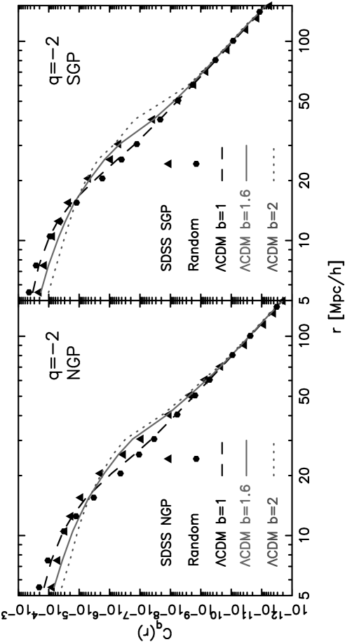
Figure 2: This shows $C_{q}(r)$ at $q=-2$ for the actual data, the random data and the simulated slices.

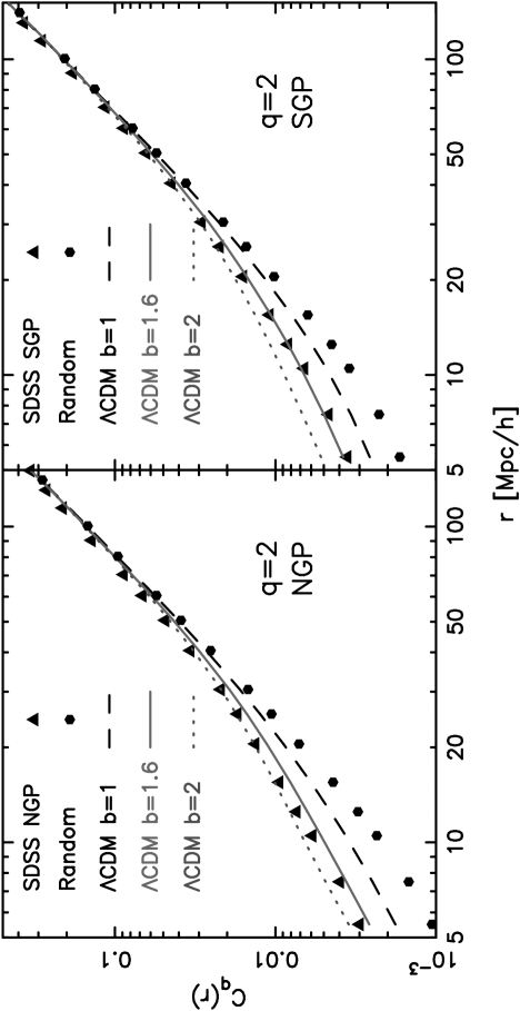
Figure 3: This shows $C_{q}(r)$ at $q=2$ for the actual data, the random data and the simulated slices.

Figures 2 and 3 show $C_{q}(r)$ at $q=-2$ and $2$, respectively, for the actual data, for one realisation of the random slices and for one realisation of the simulated slices for each value of the bias. The behaviour of $C_{q}(r)$ at other values of $q$ is similar to the ones shown here. Our analysis is restricted to $-4\leq q\leq 4$. We find that $C_{q}(r)$ does not exhibit a scaling behaviour at small scales $(5\,h^{-1}\,{\rm Mpc}\leq r\leq 40\,h^{-1}\,{\rm Mpc})$. Further, the small-scale behaviour of $C_{q}(r)$ in the actual data is different from that of the random slices and is roughly consistent with the simulated slices for $b=1.6$. We find that $C_{q}(r)$ shows a scaling behaviour on length-scales of from somewhere around $60-70\,h^{-1}\,{\rm Mpc}$ to $150\,h^{-1}\,{\rm Mpc}$. Although the actual data, the random and simulated slices all appear to converge over this range of length-scales indicating that they are all roughly consistent with homogeneity, there are small differences in the slopes. We have used a least-square fit to determine the scaling exponent or generalised dimension $D_{q}$ shown in Figure 4.

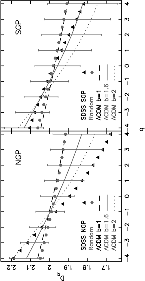
Figure 4: This shows the spectrum of generalised dimensions $D_{q}$ as a function of $q$ for the actual data, the random data and the simulated slices on length scales of from $60-70\,h^{-1}\,{\rm Mpc}$ to $150\,h^{-1}\,{\rm Mpc}$. The error bars shown are for $\Lambda{\rm CDM}$ model with bias=1.6.

Ideally we would expect $D_{q}=2$ for a two dimensional homogeneous and isotropic distribution. We find that for the actual data $D_{q}$ varies in the range $1.7$ to $2.2$ in the NGP and $1.8$ to $2.1$ in the SGP on large-scales. In both the slices the value of $D_{q}$ decreases with increasing $q$, and it crosses $D_{q}=2$ somewhere around $q=-1$. The variation of $D_{q}$ with $q$ shows a similar behaviour in the random slices, but the range of variation is much smaller $(1.9\leq D_{q}\leq 2.1)$. Comparing the actual data with the random data we find that the actual data lies outside the $1-\sigma$ error-bars of the random data (not shown here) for most of the range of $q$ except around $q=-1$ where $D_{q}=2$ for both the actual and random data. Accepting this at face value would imply that the actual data is not homogeneous at large scales.

Considering the simulated data, we find that the variation in $D_{q}$ depends on the value of the bias $b$. For the unbiased simulations $D_{q}$ shows very small variations $(1.9\leq D_{q}\leq 2.1)$ and the results are very close to those of the random data. We find that increasing the bias causes the variations in $D_{q}$ to increase. In all cases $D_{q}$ decreases with increasing $q$ and it crosses $D_{q}=2$ around $q=-1$. Increasing the bias has another effect in that it results in larger $1-\sigma$ error-bars.

Comparing the simulated data with the random data and the actual data we find that the unbiased simulations are consistent with the random data but not the actual data. The actual data lies outside the $1-\sigma$ error-bars of the unbiased $\Lambda{\rm CDM}$ model. This implies that the unbiased $\Lambda{\rm CDM}$ model has a transition to homogeneity at $60-70\,h^{-1}\,{\rm Mpc}$. The spectrum of generalised dimensions as determined from the unbiased simulations on length-scales $60-70\,h^{-1}\,{\rm Mpc}$ to $150\,h^{-1}\,{\rm Mpc}$ is different from that of the actual data ie. the unbiased $\Lambda{\rm CDM}$ model fails to reproduce the large scale properties of the galaxy distribution in our volume limited subsamples of the SDSS-DR1.

The simulations with bias $b=1.6$ and $b=2$ have larger $1-\sigma$ error-bars and these are consistent with both the random and the actual data. Interpreting the actual data as being a realisation of a biased $\Lambda{\rm CDM}$ universe, we conclude that it has a transition to homogeneity at $60-70\,h^{-1}\,{\rm Mpc}$ and the galaxy distribution is homogeneous on scales larger than this.

The galaxy subsample analysed here contains the most luminous galaxies in the SDSS-DR1. Various investigations have shown the bias to increase with luminosity (Norberg et al. 2001; Zehavi et al. 2002) and the subsample analysed here is expected to be biased with respect to the underlying dark matter distribution. Seljak et al. (2004) have used the halo model in conjunction with weak lensing to determine the bias for a number of subsamples with different absolute magnitude ranges. The brightest sample which they have analysed has galaxies with absolute magnitudes in the range $-23\leq M_{r}\leq-22$ for which they find a bias $b=1.94\pm 0.2$. Our results are consistent with these findings.

A point to note is that the $1-\sigma$ error-bars of the spectrum of generalised dimension $D_{q}$ increases with the bias. This can be understood in terms of the fact that $C_{q}(r)$ is related to volume integrals of the correlation functions which receives contribution from all length-scales. The fluctuations in $C_{q}(r)$ can also be related to volume integrals of the correlation functions. Increasing the bias increases the correlations on small scales $(\leq 40-50\,h^{-1}{\rm Mpc})$ which contributes to the fluctuations in $C_{q}(r)$ at large scales and causes the fluctuations in $D_{q}$ to increase.

The galaxies in nearly all redshift surveys appear to be distributed along filaments. These filaments appear to be interconnected and they form a complicated network often referred to as the “cosmic web”. These filaments are possibly the largest coherent structures in galaxy redshift surveys. Recent analysis of volume limited subsamples of the LCRS (Bharadwaj, Bhavsar & Sheth, 2004) and the same SDSS-DR1 subsamples analysed here (Pandey & Bharadwaj, 2004) shows the filaments to be statistically significant features of the galaxy distribution on length-scales $\leq 70-80\,h^{-1}{\rm Mpc}$ and not beyond. Larger filaments present in the galaxy distribution are not statistically significant and are the result of chance alignments. Our finding that the galaxy distribution is homogeneous on scales larger than $60-70\,h^{-1}{\rm Mpc}$ is consistent with the size of the largest statistically significant coherent structures namely the filaments.

References

- Abazajian et al. (2003) Abazajian K. et al., 2003, A J, 126, 2081
- Amendola & Palladino (1999) Amendola L., Palladino E., 1999, ApJ Letters, 514, L1
- Badii & Politi (1984) Badii R., Politi A., 1984, Physical Review Letters, 52, 1661
- Baleises et al. (1998) Baleisis A., Lahav O., Loan A.J., Wall J.V., 1998, MNRAS, 297,545
- Best (2000) Best J. S., 2000, ApJ, 541, 519
- Bharadwaj, Gupta & Seshadri (1999) Bharadwaj S., Gupta A. K., Seshadri T. R., 1999, A&A, 351, 405
- Bharadwaj, Bhavsar & Sheth (2004) Bharadwaj S., Bhavsar S. P., Sheth J. V., 2004, ApJ, 606, 25
- Baryshev & Bukhmastova (2004) Baryshev Y. V., Bukhmastova Y. L., 2004, Astronomy Letters, 30, 444
- Borgani (1995) Borgani S., 1995, Phys Reps, 251, 1
- Cappi et al. (1998) Cappi A., Benoist C., da Costa L. N., Maurogordato S., 1998, A&A, 335, 779
- Cole et al. (1998) Cole S., Hatton S., Weinberg D.H., Frenk C.S., 1998, MNRAS, 300, 945
- Coleman & Pietronero (1992) Coleman P. H., Pietronero L., 1992, Phys Reps, 213, 311
- Dekel & Lahav (1999) Dekel A., Lahav O., 1999, ApJ, 520, 24
- Efstathiou et al. (2001) Efstathiou G. et al., 2002, MNRAS, 330, L29
- Ehlers, Green & Sachs (1968) Ehlers J., Green P., Sachs R.K., 1968, J Math Phys, 9, 1344
- Guzzo (1997) Guzzo L., 1997, New Astronomy, 2, 517
- Hawkins et al. (2003) Hawkins E. et al., 2003, MNRAS,346,78
- Hatton (1999) Hatton S., 1999, MNRAS, 310, 1128
- (19) Hogg D. W., Eistenstein D. J., Blanton M. R., Bahcall N. A., Brinkmann J., Gunn J. E., Schneider D. P., 2004, Submitted to ApJ,(astro-ph/0411197)
- Kaiser (1984) Kaiser N., 1984, ApJ Letters, 284, L9
- Kurokawa, Morikawa & Mouri (2001) Kurokawa T., Morikawa M., Mouri H., 2001, A&A, 370, 358
- Lahav (2002) Lahav O., 2002, Classical and Quantum Gravity, 19, 3517
- Lin et al. (1996) Lin H., Kirshner R. P., Shectman S. A., Landy S. D., Oemler A., Tucker D. L., Schechter P. L., 1996, ApJ, 471, 617
- Martínez, López-Martí, & Pons-Bordería (2001) Martínez V. J., López-Martí B., Pons-Bordería M., 2001, ApJ Letters, 554, L5
- Mo & White (1996) Mo H.J., White S.D.M., 1996, MNRAS, 282, 347
- Nusser & Lahav (2000) Nusser A., Lahav O., 2000, MNRAS, 313, L39
- Norberg et al. (2001) Norberg P. et al., 2001, MNRAS, 328, 64
- Pandey & Bharadwaj (2004) Pandey B., Bharadwaj S., 2005, MNRAS, 357, 1068
- Pan & Coles (2000) Pan J., Coles P., 2000, MNRAS, 318, L51
- Peebles (1980) Peebles P.J.E., 1980, The Large-Scale Structures of the Universe, Princeton University Press, Princeton, NJ
- Percival et al. (2001) Percival W. J. et al., 2001, MNRAS, 327, 1297
- Percival et al. (2002) Percival W. J. et al., 2002, MNRAS, 337, 1068
- Pietronero (1987) Pietronero L., 1987, Physica A, 144, 257
- Scharf et al. (2000) Scharf C. A., Jahoda K., Treyer M., Lahav O., Boldt E., Piran T., 2000, ApJ, 544, 49
- Spergel et al. (2003) Spergel D. N. et al., 2003, ApJ, 148, 175
- Sutherland & Efstathiou (1991) Sutherland W., Efstathiou G., 1991, MNRAS, 248, 159
- Taruya & Suto (2001) Taruya A., Suto Y., 2001,ApJ, 542, 559
- Tegmark et al. (2004a) Tegmark M. et al., 2004, PRD, 69, 103501
- Tegmark et al. (2004b) Tegmark M. et al., 2004, ApJ, 606, 702
- Tucker et al. (1997) Tucker D. L. et al., 1997, MNRAS, 285, 5
- Seljak et al. (2004) Seljak U. et al., 2005, PRD, 71, 043511
- Wu, Lahav & Rees (1999) Wu K., Lahav O., Rees M., 1999, Nature, 397, 225
- Yoshikawa et al. (2001) Yoshikawa K., Taruya A., Jing Y.P., Suto Y., 2001, ApJ, 558, 520
- Zehavi et al. (2002) Zehavi I. et al., 2002, ApJ,571,172