Radio-Detection Signature of High Energy Cosmic Rays by the CODALEMA Experiment

Abstract

Taking advantage of recent technical progress which has overcome some of the difficulties encountered in the 1960’s in the radio detection of extensive air showers induced by ultra high energy cosmic rays (UHECR), a new experimental apparatus (CODALEMA) has been built and operated. We will present the characteristics of this device and the analysis techniques that have been developed for observing electrical transients associated with cosmic rays. We find a collection of events for which both time and arrival direction coincidences between particle and radio signals are observed. The counting rate corresponds to shower energies $\geq 5\times 10^{16}$ eV. The performance level which has been reached considerably enlarges the perspectives for studying UHECR events using radio detection.

1 Introduction

For almost 70 years, physicists and astronomers have studied cosmic rays and gained a good knowledge of the flux as a function of energy up to $10^{19}$ eV. However, in this energy range, the problem of the origin and the nature of ultra-high energy cosmic rays (UHECR) is unsolved and stands as one of the most challenging questions in astroparticle physics. In order to collect the elusive events above $10^{19}$ eV (which present an integrated flux of less than 1 event per km² per steradian and per year) giant detectors are needed and are presently being designed and built. Today, for studying the highest energy extensive air showers (EAS), a leading role is played by the Pierre Auger Observatory [1] which uses a hybrid detection system combining particles and fluorescence which inherently have very different duty cycles. An alternative method was suggested long ago by Askar’yan [2] consisting in the observation of radio emission associated with the development of the shower. This method is based on the coherent character of the radio emission and deserves, in our opinion, serious reinvestigation due to many potential advantages as compared to other methods. Besides expected lower cost and sensitivity to the longitudinal shower development, it primarily offers larger volume sensitivity and duty cycles which can result in higher statistics, thus offering better possibilities to discriminate between postulated scenarios of UHECR nature and origin [3].

Experimental investigations carried out in the 1960’s proved the existence of RF signals initiated by EAS (for a comprehensive review see [4]). The evidence was obtained with systems consisting either of a radio telescope or an antenna, sometimes a few antennas, triggered by particle detectors. The bulk of the data was obtained in narrow frequency bands (about 1 MHz), centered around various frequencies in the 30–100 MHz range. The difficulties encountered were numerous. Among other things, insufficient electronics performance and problems due to atmospheric effects led to poor reproducibility of results, and this area of research was abandoned in favour of direct particle [5] and fluorescence [6] detection from the ground.

But in recent years, the idea has once again come to the forefront and new experiments have been undertaken to detect radio pulses and measure their characteristics. In one case, motivated by the perspective of large-scale cosmic ray experiments, data were taken with a single antenna put into coincidence with the CASA-MIA detector [7]. In another case, in the perspective of the next generation of low-frequency radio telescopes [8, 9], an array of antennas was deployed to run in coincidence with the KASCADE air-shower detector [10].

In this paper, we report on studies conducted with a radio air shower detector using a multi-antenna array [11, 12, 13] set up at the Nançay radioastronomy observatory. From the earlier radio detection experiments, several criteria were retained to provide optimal conditions for the detection of transients: choice of a radio-quiet area, a well-understood radio frequency (RF) electromagnetic environment, the use of several antennas in coincidence and broadband frequency measurements. After a discussion, in section 2, of the characteristics predicted for the electric pulses generated by EAS, section 3 will describe the CODALEMA (COsmic ray Detection Array with Logarithmic ElectroMagnetic Antennas) experiment together with the trigger definition in stand-alone mode. Observation of transient signals are discussed in section 4 and the analysis techniques are outlined in 5 along with their limitations. Particle detectors have been set up to provide a trigger on cosmic ray events. After a description of the analysis carried out in this mode of operation, section 6 shows that some of the observed transients originate from EAS. Conclusions and perspectives are given in the last section.

2 Signal properties

An extensive air shower contains a huge number of electrons and positrons (several billion at maximum for $10^{20}$ eV). At first glance, the stochastic nature of such moving charge distributions should produce incoherent fields. This is the case for the Čerenkov radiation visible in the optical domain. It turns out, however, that several physical effects systematically break the symmetry between the electron and positron distributions inside the shower, leading to a coherent field contribution in the RF domain. This is the case for the so-called Askar’yan emission [2] for which Compton scattering and in-flight positron annihilation create an excess of electrons in the shower front. In a recent experiment [14] in which a GeV photon beam was sent into a sand target several meters long, this coherent emission was observed and its properties were found to be consistent with the predictions. Based on this phenomenon, radio detection of cosmic ray induced showers in dense media is currently under investigation [15, 16]. The Askar’yan effect should also exist for EAS, though it is likely to be dominated by the coherent emission associated with another charge separation mechanism, charge deflection in the Earth’s magnetic field [4, 17, 18].

2.1 Electric field characteristics

In order to determine the feasibility of measuring electric fields from high energy air showers, it is first necessary to have some estimates for the maximal amplitude and the time scale(s) of the associated signal as well as their lateral distribution at ground level.

2.1.1 Around $10^{20}$ eV

For a set of widely spaced antennas, most events will be at large impact parameters. In this range, the time scale is primarily set by the time development of the shower albeit with a certain amount of Doppler contraction. Time differences between signals from different individual charges at a given shower age are generally small on the above time scale. Consequently, a good assumption is provided with a point-like charge approximation. The interest of such a model is that electric field behavior is easy to obtain with standard textbook formulas [4, 19].

The easiest field contribution to evaluate is that due to charge excess [2]. In principle, the excess is a function of particle energy, but this effect can be ignored in a first estimate. Thus, $q(t)=-\varepsilon N(t)e$, with $N(t)$ the number of electrons at a given time and $\varepsilon$, the fractional excess. At an observation point $A$ and at time $t$, the electric field for a moving point-like charge is given by

$$\mathbf{E}(t,A) = \frac{1}{4\pi\epsilon}\sum_{t^{\prime}}(1-v^{2}/c^{2})q\frac{\mathbf{R}-R\mathbf{v}/c}{|R-\mathbf{R}\cdot\mathbf{v}/c|^{3}}$$ (1)

$$+\frac{1}{4\pi\epsilon c}\sum_{t^{\prime}}\dot{q}\frac{\mathbf{R}-R\mathbf{v}/c}{(R-\mathbf{R}\cdot\mathbf{v}/c)|R-\mathbf{R}\cdot\mathbf{v}/c|}$$

where $\mathbf{R}=\overrightarrow{QA}$ is the vector between the charge position at time $t^{\prime}=t-R/c$ and the observation point and $\mathbf{v}$ is the charge velocity.

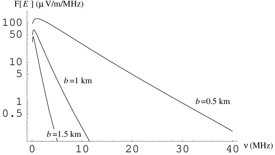
Figure 1: Top panel: electric field as a function of time for various impact parameters at sea level for a $10^{20}$ eV vertical shower with $\varepsilon=10\%$ and $Xmax=1700$ m. Bottom panel: corresponding magnitude coefficient distributions obtained from the Fourier transforms.

In the upper part of Fig. 1, the horizontal component of the electric field is plotted as a function of time for a $10^{20}$ eV vertical shower ($\varepsilon=10\%$, $Xmax=1700$ m) with impact parameters $b=0.5$, 1 km and 1.5 km . At $b=1$ km the field reaches 230 $\mu$V$/$m. Such sizable values can be obtained only for huge cosmic ray energies. This points also to the fact that long distance detection is only possible for extremely high energies. The lower part of Fig. 1 presents the associated Fourier spectra indicating that very broadband antennas must be used in order to maintain sufficient sensitivity in the MHz range. The coherence, which is essential in order to reach such high values, is lost at high frequency where the structure of the shower becomes resolved. These limitations are moderated somewhat in the case of inclined shower configurations [20] and by the fact that for most shower orientations the dominant field contribution is likely to come from charge deflection in the Earth’s magnetic field [4, 17, 18].

An inspection of Eq. (1) shows that the electric field waveform gives an image of the longitudinal development of the shower. In this respect, the information obtained by the radio technique is comparable to that of fluorescence detectors, though this radio image is distorted by the Doppler effect and by the ultra-relativistic nature of the emitting charges.

2.1.2 Around $10^{17}$ eV

Because the rate of $10^{20}$ eV cosmic rays is very small, an experiment would need a setup covering a large surface in order to collect enough statistics. Consequently it has been decided to work at much lower energy. Because the energy radiated through coherent emission is expected to be proportional to the square of the number of charges within the shower (i.e. proportional to the square of the energy of the primary), signals from $10^{17}$ eV air showers will be appreciably smaller than at $10^{20}$ eV. At large distance from the shower core, this effect will be strengthened. Therefore, the contribution to the rate from EAS will be dominated by those whose cores fall within (or close to) the area delimited by the antennas and with a small number of antennas, interesting events are likely to be those that are detected by the majority, if not all, of them. Taking into account the inter-antenna distance of our setup (see 3), an estimate of the electric field must be made for impact parameters in the 100 meter range. In this domain of impact parameters, no simple expression for the electric field can be given. Recent modelizations exist regarding this question [18, 22], but here we will use estimates as provided in Refs. [4] and [7].

The pulse waveform can be written

$$f(t)=\theta(t)Ae^{2}\left(\frac{t}{2\tau_{1}}\right)^{2}\left(e^{-t/\tau_{1}}-(\tau_{1}/\tau_{2})^{3}e^{-t/\tau_{2}}\right),$$ (2)

where $\theta(t)=1$ for $t>0$ and $0$ for $t<0$. This expression is derived from various general considerations concerning the shower’s electric field. In particular, the second exponential represents a negative-amplitude component such that the signal has no DC component. Its duration is, at least for a vertical shower, much longer than the positive-amplitude component ($\tau_{2}\gg\tau_{1}$) and is, therefore, of minor importance for the present discussion. For $\tau_{2}\gg\tau_{1}$ the relevant parameters are thus $\tau_{1}$ which fixes the time scale of the positive-amplitude part (the maximum is reached at time $t=2\tau_{1}$) and $A$ the maximum amplitude.

For a $10^{17}$ eV vertical shower at small impact parameters, Allan [4] estimates the pulse duration to be of the order of 10 ns and the electric field amplitude $A\sim 150$ $\mu$V$/$m. The pulse waveform from Eq. (2) with $\tau_{1}=2$ ns, $A=1$ and $\tau_{2}=10\times\tau_{1}$, and the corresponding modulus of the Fourier transform are shown in Fig. 2.

2.2 Filtering and triggering

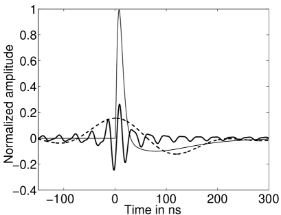
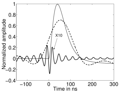
Figure 3: Raw pulses (thin line) and their band-pass filtered counterparts for bandwidths of 30–60 MHz (thick full line) and 1–5 MHz (dashed line).

From the experimental point of view, the electrical signal will be distorted when passing through the detector chain consisting of elements such as antennas, cables and preamplifiers. Insertion losses and filtering effects will decrease the signal amplitude and strongly modify the initial waveform. The effect of band-pass filtering is shown in Fig. 3 for a short duration pulse such as that of Fig. 2 as well as a much longer one.

Whatever the duration of the pulse may be, the high frequency component (30–60 MHz) is correlated with the rise time of the signal and is suitable for trigger purposes. In addition, depending on its duration, analysis of the low frequency part of the signal (1–5 MHz) can lead to a direct estimate of the signal amplitude.

The capability to detect the radio signal strongly depends on the choice of the frequency band. Nevertheless, the simultaneous presence of the time-limited oscillating signals in two widely separated frequency bands enables us to distinguish broadcast emissions, which are quasi-monochromatic, from broadband signals such as the ones expected from EAS.

3 The experimental set-up

One of the originalities of CODALEMA lies in the fact that the system can be self-triggered using a dedicated antenna, as opposed to the other experiments mentioned above where particle detectors provide the triggering. However, for such an experiment, it is then necessary to become acquainted with the characteristics of the transient RF sky, which, in addition, is almost completely unexplored for time scales ranging from nanoseconds to microseconds. The decision was made to tackle the problem with a small number of antennas arranged in a “self-triggered all-radio” system, intrinsically suited to measuring the RF transient rate. We expected this task to be facilitated by the progress accomplished in electronics and data processing since the 1960’s. In the meantime however, the sky has generally become much noisier than at the time of the pioneering work. Thus the only condition imposed for recording data is the arrival of a suitable RF transient on a trigger antenna, provided that the dead time due to the data recording (i.e. the trigger rate), stays at an acceptable level. Under these conditions, the duty cycle stays close to 100% and the setup should be well suited for registering possible incoming EAS signals.

An alternative strategy would have been to design a system where antenna signals are sampled when a particle trigger occurs. In fact this method, which has its own physical limitations, is now being used [21] and will be described in 6. However, for such designs the sky transient background is inaccessible because the overall observation time remains very small: as an example the time window ($50~{}\mu$s) which is used in [7] in association with the low particle-trigger rate, leads to an integrated observation time of only a small fraction of a second (50 ms), for a typical day-long run.

3.1 General layout

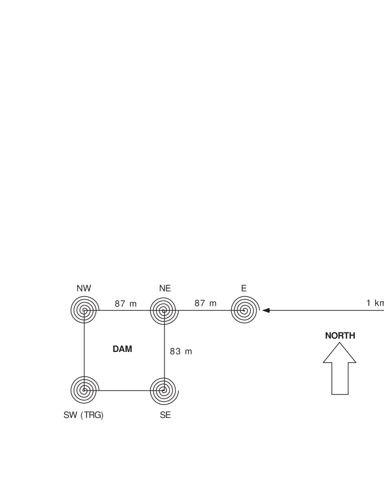
Figure 4: The CODALEMA setup, first phase.

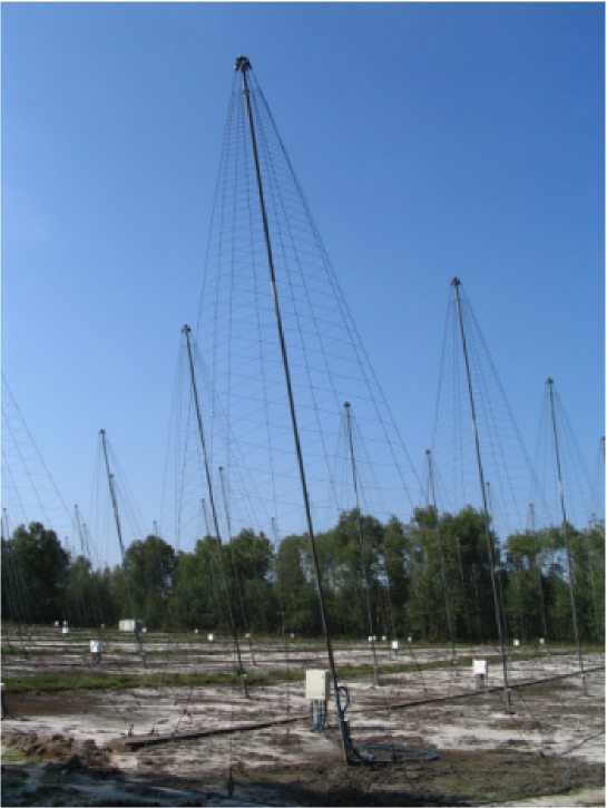
Figure 5: Photograph of the logarithmic antennas of the Nançay DeCAmetric Array. The CODALEMA experiment uses some of these antennas.

Running from March 2003, the CODALEMA experiment in its first phase used 6 of the 144 log-periodic antennas of the DecAMetric array (DAM)(see figure 5), an instrument dedicated to the observation of the sun and Jupiter based at the Nançay Radio Observatory [23]. Having 1–100 MHz frequency bands, these antennas are well adapted to our sensitivity and frequency requirements. The antenna locations are shown in Fig. 4.

Four of the antennas, namely NE, SE, SW and NW, are located at the corners of the DAM array. This layout was chosen in order to have distances between detectors as large as 120 m and to minimize the cable lengths. Two additional antennas, namely E and Distant, were setup to the east of the DAM at respectively 87 m and 0.8 km providing longer inter-antenna distances. From the information on the electric field strength far from the central array, it is possible to identify and eliminate broadcast signals and strong interference phenomena (storms, etc.), expected to irradiate widely-separated antennas with more or less uniform power.

RF signal amplification(1–200 MHz, gain 35 dB) is performed using commonly available low-noise electronic devices which have a negligible impact on the overall noise of the electronic chain. The five grouped antennas are linked via 150 m coaxial cables (RG214U) to LeCroy digital oscilloscopes (8 bit ADC, 500 MHz frequency sampling, 10 ${\mu}$s recording time). The Distant antenna requires a different signal transmission technique, an optical fiber link approximately 1 km long which introduces significant attenuation (a factor of 10), a 5.5 ${\mu}$s delay as well as a low frequency cutoff at 10 MHz from the analog/optical transceiver. Special attention is paid to the shielding both of the electronics itself and the acquisition room in order to minimize interference coming from data-taking activities.

3.2 Trigger definition

A trigger with minimum bias was chosen in order to select potentially interesting events. It is sensitive to the unusual frequency contributions which come from transient signals. The amplitudes of these contributions are compared to the normal sky background level, whose frequency content has been precisely measured on site with one of the antennas using the complete acquisition chain. The power spectral density from this measurement is shown in Fig. 6. Above 90 MHz, peaks associated with FM radio signals are clearly observed. Between 20 MHz and 90 MHz, a rather quiet band is found reaching $10^{-3}$ V/MHz. Below 20 MHz, numerous transmitter spectral lines result, with our spectral resolution, in a quasi continuous contribution far above the minimum. Nevertheless, a quieter band ($\simeq 2.10^{-3}$ V/MHz) can be found between 1 MHz and 5 MHz as shown in the inset of Fig. 6. Evaluations of the noise characteristics have also been done in several other places showing that the spectral profile depends strongly on the experimental location. For example, the CASA-MIA collaboration in the Utah desert observed interference at 55 MHz from a TV transmitter over 100 km away. However, concerning the Pierre Auger Observatory site [24] (Malarg e, Argentina), we recently monitored the R.F. sky there and found that in the frequency windows of interest it is as clean as the Nançay site. Thus the main constraints come from the proximity of human activities, and a significant advantage of places such as Nançay and the Auger site is to present very quiet environments.

As explained in section 2, the frequency distribution of the expected transients shows a wide band contribution. A signal reaching the setup will add its frequency contributions to the noise frequency distribution. Due to the structure of the noise spectrum, the resulting effect will be more easily seen in the two quiet bands discussed above, with the better signal to noise ratio obtained for the 20–90 MHz range. Moreover, for timing considerations, it is also important to find a quantity which will determine the arrival time of the signal. Based on the information presented in Fig. 3, the maximum absolute value of the oscillating high frequency filtered signal, which is strongly correlated to the leading edge of the signal, was chosen. In addition, because the associated error is then related to the pseudo period of the oscillations, the higher the filtering frequency, the lower the uncertainty is. Taking into account these considerations, it was thus decided to use only part of the 20–90 MHz range, namely 33–65 MHz, for the trigger antenna. The quiet 1–5 MHz band may then be used to quantify the low frequency contribution of any wide band signal.

To generate the trigger, the signal of the antenna chosen for this purpose is sent through an analog band-pass filter (33–65 MHz) to its corresponding oscilloscope channel. An internal leading-edge discriminator condition applied to this channel sets the amplitude threshold used to initiate data recording. For each trigger sequence, the data from all the antennas are stored on disk for off-line analysis.

3.3 Field sensitivity

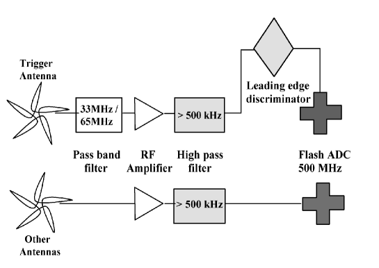
Figure 7: CODALEMA electronics chain.

The electronics setup used is shown in Fig. 7. Following RF amplification, all the signals go through a high-pass filter ($\geq$ 500 kHz) to remove the contribution of an AM transmitter (164 kHz) located 22 km south of Nançay. The signal is digitized using a 8-bit ADC at a sampling frequency of 500 MHz with a 10 ${\mu}$s recording time. Broadband waveforms are recorded for all the antennas but the trigger, for which the 33–65 MHz band-pass filter is present as indicated above. For the other antennas, two different broadband configurations have been used during the experiment. The antenna sensitivity rapidly decreases above 100 MHz, thus for analysis purposes, the “full band” configuration has been restricted to 1–100 MHz and has been used to search for low frequency counterparts of the transients. The “restricted band” configuration (analog filtering between 24 and 82 MHz) presents a better signal-to-noise ratio and has been devoted to the search of weak transients. Table 1 indicates the sensitivity reached by the apparatus for the different configurations.

This trigger sensitivity has to be compared with the expected value for a $10^{17}$ eV vertical shower with a small impact parameter. The values chosen for $A$ and $\tau_{1}$ are respectively 150 $\mu$V$/$m and 2 ns (see section 2.1.2). At this energy, in the frequency band $\nu_{0}\pm\Delta\nu/2=50\pm 15$ MHz, the expected field should give a peak amplitude

$$E_{\mathrm{pk}}=2|S(\nu_{0})|\Delta\nu=55\ \mu\mathrm{V/m}$$

where $S(\nu_{0})$ is the Fourier transform at frequency $\nu_{0}$ (see Fig. 2).

This gives a voltage amplitude on the terminal resistance $R=50~{}\Omega$  [7, 25]

$$V_{\mathrm{pk}}=E_{\mathrm{pk}}\frac{c}{2\nu_{0}}\sqrt{\frac{RG}{\pi Z_{0}}}=2\ \mathrm{mV}$$

where $Z_{0}=377~{}\Omega$ and $G$ is the overall gain from the antenna to the terminal resistance including the antenna gain ($7$ dB), the amplifier gain ($35$ dB) and the attenuation of the line ($-7$ dB). These values clearly show that the electronic sensitivities in this frequency band are adapted to the requirements for detecting EAS.

Concerning the trigger, it had been found that the background sky noise at Nançay, referred to as $\sigma_{sky}$ in this paper, has a standard deviation of 0.5 mV within the frequency band of interest. In order to exclude most of the noise, we chose to set the leading edge discriminator threshold to a value greater than $4\,\sigma_{sky}=2$ mV which, as shown above, sets the lower energy limit for detection to around $10^{17}$ eV.

This setup was operated on a regular basis between March 2003 and June 2004. During that time $3.2\times 10^{3}$ hours of running time corresponding to $5.1\times 10^{4}$ triggers were accumulated, mostly devoted to setup and optimization of the device (electronics, trigger antenna position, trigger threshold,… ). However, during the last six months of this period, data were taken for the sole purpose of physics observations. The “Full band” configuration (see table 1) was used for most of the runs with a trigger threshold ranging from 4 to 10 mV. These runs were devoted to the search for strong electric field pulses in the microsecond range coming either from the sun, Jupiter or storms. These data are currently under analysis. In June 2004, runs devoted to searching for radio emission from EAS were carried out (see next section). Filters were installed on all except the trigger antenna in order to increase the sensitivity (“restricted band” configuration) and the trigger threshold was set to 2 mV.

4 Transient signals

4.1 Trigger rates

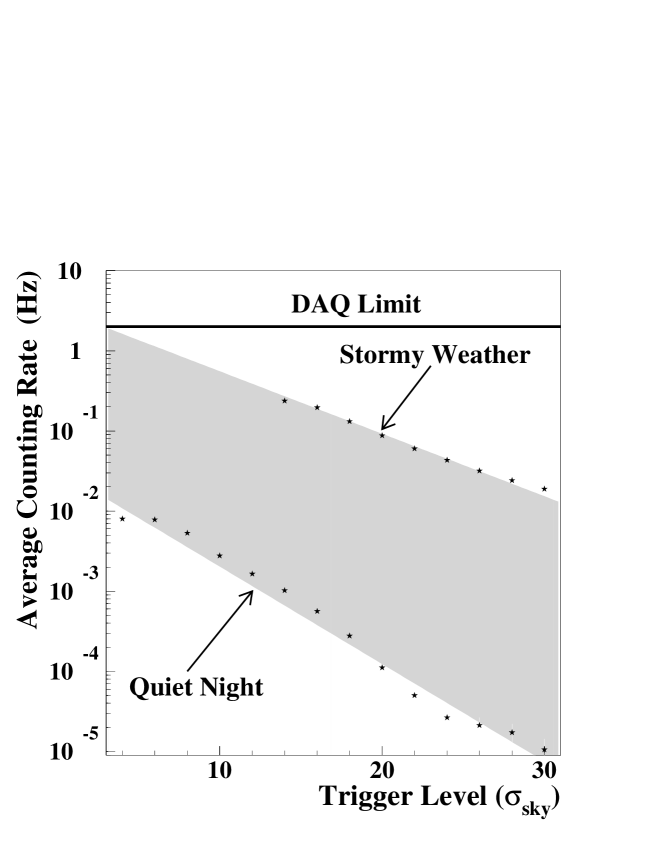
Figure 8: Evolution of the counting rate as a function of the discriminator threshold.

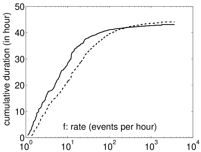
Figure 9: Cumulative running time at a rate smaller than $f$ as a function of the instantaneous rate $f$, for events with several antennas in coincidence (full line) and for all registered events (dashed line)

In Fig. 8 the average counting rate at Nançay is presented as a function of the trigger level, expressed in units of $\sigma_{sky}$. The counting rate evolves greatly with human activities in the vicinity of the station as well as with the weather conditions. The shaded area corresponds to the measured counting rates. The lower limit was obtained during quiet night runs whereas the upper one corresponds to stormy weather. Even then, the acquisition system’s maximum rate of two events per second is rarely reached. During the quietest nights very low counting rates were obtained, making possible the detection of electric fields as low as 50 $\mu$V$/$m. Among the events recorded, only a few correspond to an electromagnetic (EM) wave crossing the apparatus. In order to identify these events, we have compared two event configurations: one using all the recorded events, the second presenting coincidences between the TRG, SE and NW antennas. The procedure used to process the signals from the antennas is presented in section 5. The cumulative running time obtained with this criterion is shown in Fig. 9 as a function of the instantaneous rate $f$ which is defined as $f=\frac{1}{\Delta t}$, where $\Delta t$ is the time between two consecutive events. The figure includes a total of 44 hours of data-taking time at a threshold level of 4 $\sigma_{sky}$.

As can be seen, for both event topologies, the rate was smaller than 10 events per hour for a total of about 30 hours. These values can be compared with the background rates observed in Ref. [7], where the first level selection gives an average of more than one transient every 50 $\mu$s. Though occasional counting rates greater than one or two Hz cannot be excluded with the present setup, Fig. 9 shows that there are large radio-quiet time intervals. The conclusion is therefore that the sky at Nançay during the frequent quiet periods is almost free of electrical transients, even with a low trigger threshold, thus offering excellent conditions for detecting EAS.

4.2 Waveform observation

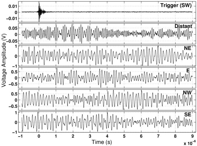
Figure 10: Waveforms from the six antennas for a typical event. The trigger antenna is filtered while the others are wide-band (see text).

In Fig. 10 the signal waveforms are shown for all the antennas for a typical event. The trigger pulse determines the origin of the time scale. Due to the variable time-of-flight of the EM signal (the contribution from cosmic rays corresponding to an isotropic primary flux), the time involved in generating the trigger and the effects of cable length, antenna pulses may precede the trigger signal. Consequently, the oscilloscopes were set up to have a 1 $\mu$s pre-trigger time. The trigger trace shows an oscillating pulse due to the band-pass filter on this antenna as seen in section 2.2. For all the other antennas, the expected signal is hidden by the combined contributions from the radio transmitters.

5 Signal processing

The first stage of the offline analysis is to find evidence for a transient signal in the wide band channels and to determine its associated time. Then the arrival direction of the incident electric field is deduced if a coincidence is observed involving several antennas. Based on shower properties, it is then possible to define criteria for our device to select events from EAS. Finally in view of a future step of the analysis, a possible method to recover the waveform of the original signal is presented.

5.1 Observation of coincidences

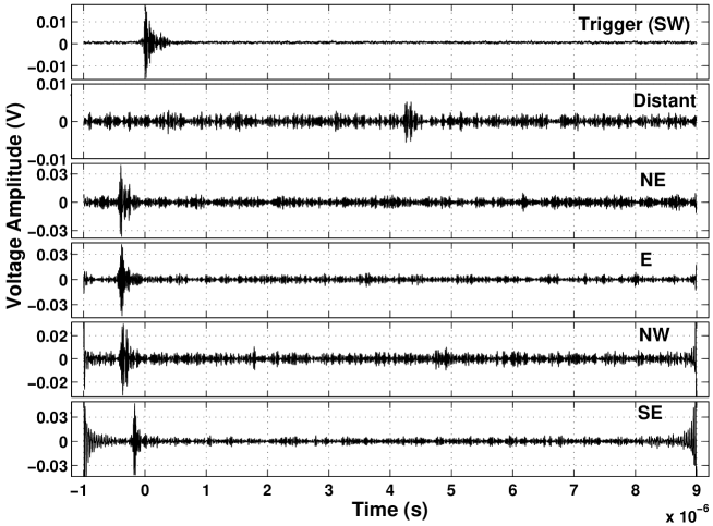
Figure 11: Coincident transients in the 33–65 MHz band obtained using numerical filtering for the event presented in figure 10.

In order to reduce the broadcast contributions, we have filtered the data numerically using the same frequency band as for the trigger (33–65 MHz). Such a procedure is expected to enhance the presence of any existing wide band signals. The effect of this band-pass filtering is shown in Fig. 11 for the same event as in Fig. 10. At each end of the time range, spurious oscillations, coming from the Gibbs phenomenon, are further removed by eliminating the two signal extremities (400 ns). In the remaining time window, all antennas show a short oscillating signal, which is characteristic of the result of band-pass filtering on a transient pulse. The timing differences correspond to the propagation times of the wavefront to the different antennas, and also include electronics and cable delays. The signal detected on the Distant antenna (0.8 km from the others) shows that transients can be observed over large distances with our setup.

The major advantage of wide band data acquisition is the possibility to filter the signal off-line in any desired frequency band. In our case, the low (1–5 MHz) band should be a valuable frequency window (see section 3.2) to provide additional indications of the presence of broadband transients. However the limited performance of the ADCs (8 bits) and the bandwidth of the amplifiers used in this phase of the experiment have not yet permitted us to perform such analysis. Currently, new 12 bit ADCs are being installed, and after this upgrade it should be possible to investigate this technique.

5.2 Procedure for transient identification

In order to determine whether a transient pulse is present from a particular antenna, we follow the filtering procedure just described. A threshold is then set such that the signal voltage is required to exceed the average noise, estimated on an event-by-event basis. This approach takes into account differences due to antenna location as well as variations in radio conditions resulting from atmospheric perturbations and human activities.

As already mentioned, filtering the pulse generates an oscillating pattern. In order to treat the positive and negative parts on an equal footing, we use an antenna pulse power variable $P_{i}=v_{i}^{2}$ where $i$ is a time index with steps of 2 ns ($i=1$–5000) and $v_{i}$ is the band-pass filtered pulse voltage at time $i$. The procedure is as follows:

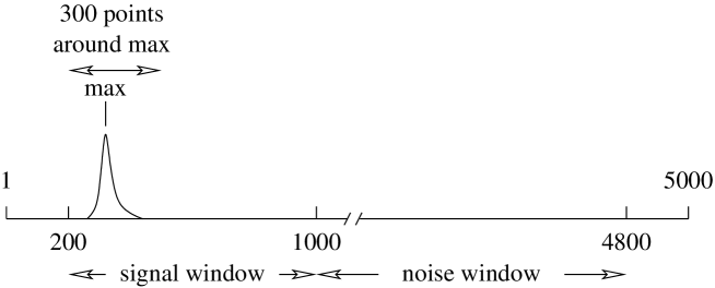
Figure 12: Time windows used for the determination of signal and noise. The power average is calculated using the interval $[i_{\mathrm{max}}-150:i_{\mathrm{max}}+150]$. When the maximum is close to the edge of the signal window, we use either the $[200:500]$ or the $[700:1000]$ interval.

• the time range is divided into a signal window ($i=200$–1000) and a noise window ($i=1000$–4800) (see Fig. 12);

• in the noise window, the noise average $\mu_{n}=\langle P\rangle_{\mathrm{noise}}$ and the standard deviation $\sigma_{n}=\sqrt{\langle(P-\mu_{n})^{2}\rangle_{\mathrm{noise}}}$ are calculated;

• a pulse transient is flagged when the power average $\mu_{s}=\langle P\rangle_{\mathrm{signal}}$ in a 300-point time range encompassing the $P_{i}$ maximum in the signal window (see Fig. 12) is significantly greater than $\mu_{n}$, namely:

  $$\mu_{s}\geq\mu_{n}+k\frac{\sigma_{n}}{\sqrt{N_{s}}},$$

  where $N_{s}$ is the number of points in the time window. The number $k$ has been adjusted empirically and $k=10$ has been found to provide unambiguous rejection of signals that are not pulse-like.

5.3 Time tagging and triangulation

The electromagnetic propagation time from one antenna to another 100 m away is at most 330 ns (for a horizontal wave). This sets the scale for the delays between two neighboring antennas in the network (excluding the Distant antenna). Due to signal shrinking by Doppler contraction, the pulse rise-time is expected to be small on this time scale. The choice of a particular point on the waveform, e.g. maximum or 10% of the maximum, is therefore not a critical issue in obtaining a reference time. Taking advantage of the correlation that exists between the leading edge of the pulse and the maximum of the oscillation envelope of the filtered signal (see Fig. 3), the pulse arrival time is taken to be the point at which $P=v^{2}$ is maximum in the filtered band. The time determination uncertainty due to the filtering is given by half the pseudo-period of the filtered signal and is thus smaller than 20 ns.

The arrival times from the various antennas can then be used to determine the incident direction of the electromagnetic wave. With the hypothesis of a far source (at $10^{17}$ eV, vertical showers have their maxima at an altitude of several km), a plane-wave approximation is appropriate. The plane’s orientation is determined by a fitting procedure and requires at least three coincident antennas, since the following relation exists between arrival times $t_{j}$, and antenna positions $(x_{j},y_{j},z_{j})$:

$$ct_{j}=\alpha x_{j}+\beta y_{j}+\gamma z_{j}+ct_{0},$$

where $(\alpha,\beta,\gamma)$ is the unit vector giving the EM field incidence direction and $t_{0}$ the (unknown) time at which the wavefront plane crosses the origin of the $(x,y,z)$ frame. Since, for the flat Nançay site, the antennas are considered to lie in a horizontal plane, we take $z_{j}=0$, and $\gamma$ cannot be determined directly. The other parameters $\alpha,\beta$ and $t_{0}$ are calculated using a least square fit to minimize the quadratic error

$$\epsilon^{2}=\frac{1}{n_{\mathrm{trig}}}\sum_{j}f_{j}\times(ct_{j}-\alpha x_{j}-\beta y_{j}-ct_{0})^{2}$$

where $f_{j}$ is 1 or 0 depending on whether a transient is flagged or not on antenna $j$, and $n_{\mathrm{trig}}=\sum f_{j}$. When $n_{\mathrm{trig}}\geq 4$ the value of $\epsilon$ gives the residual error. When coincidences occur that involve at least four antennas it is possible to fit to a spherical wavefront instead of to a plane. However, for a point source located at a distance $R$, much larger than the antenna separation $\Delta$, the correction is of the order of $\Delta^{2}/R$. This is larger than 10 m for $\Delta\sim 100$ m only if $R\leq 1$ km so we consider the plane fit to be quite sufficient for the air showers of interest.

The zenith ($\theta$) and azimuthal ($\varphi$) angles are determined by inverting the relations

$$\alpha=\sin\theta\cos\varphi,\quad\beta=\sin\theta\sin\varphi.$$

5.4 Event reconstruction

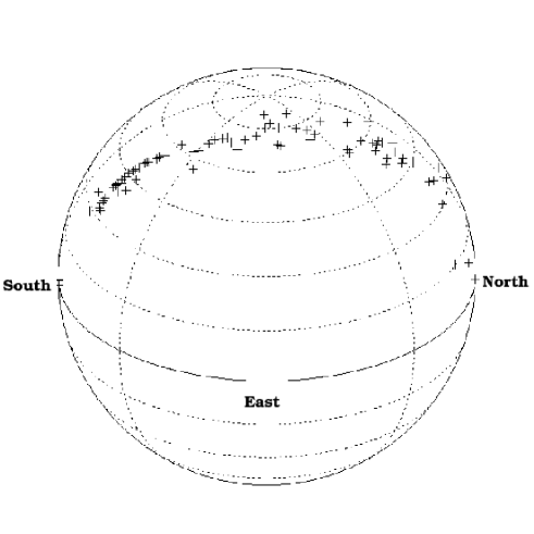
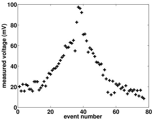
Figure 13: Up: Location in the sky of the mobile source. Down: Maximum voltage recorded on one of the antennas during this series of triggers.

The capability of the device to reconstruct signal directions is illustrated below using a somewhat atypical data set recorded by CODALEMA consisting of nearly a hundred successive triggers that occurred within a 2 minute period. This high trigger rate would suggest that those events are from interference of human or atmospheric origin. In Fig. 13 the wavefront direction for each event is plotted on a sky map. The sequence of points form a trajectory which would correspond to that of a single emitting source moving from north to south above the detector array.

The maximum measured voltage on one of the antennas for this event sequence is plotted to the right in Fig. 13. As expected for a single source moving on a more or less linear trajectory above the detector, the maximum measured voltage increases as the source approaches, then decreases when it moves away. The interpretation of these observations is that the source is an aircraft or possibly a satellite passing over Nançay.

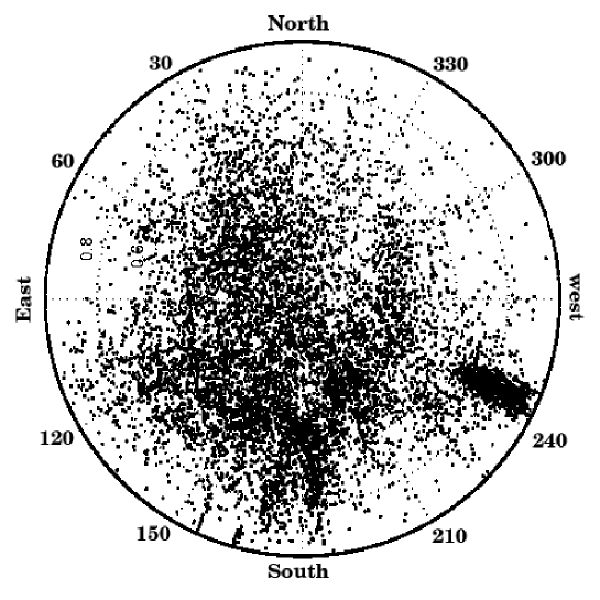
Figure 14: Projection on the ground plane of the directions of $11\times 10^{3}$ reconstructed events among the $50\times 10^{3}$ recorded by CODALEMA between March 2003 and June 2004. An accumulation of events close to the horizon is visible from the West-South-West dues to human activities in the vicinity of the station.

Fig. 14 shows the directional distribution of the 11000 reconstructed events resulting from a year of data taking.

A substantial number of events had a below-horizon direction and are not plotted in the figure. With the help of a spherical fit, most of these were found to originate from electrical devices located at various points on the Nançay observatory site. For the reconstructed events in the plot, their distribution indicates that the detector array has higher sensitivity for signals coming from the south. This is not surprising since the antennas are inclined to the south (tilting of $25^{\circ}$) to facilitate observations of the sun and Jupiter.

5.5 Event selection

Due to the steep falloff of the cosmic ray flux with energy, most of signals that produce a trigger should correspond to 10¹⁷ eV EAS (see section 2.1.2). Based on the properties of these showers, any such events must fulfill several conditions. At this energy, showers with small impact parameters, i.e. whose axis is close to or inside the square formed by the four DAM antennas, are expected to provide the largest signal amplitudes. As a consequence, the presence of tagged signals on the four antennas constitutes the first experimental criterion (referred to as “square”) required to select events from EAS. In addition, the distant antenna would only be tagged by very energetic and very unlikely events or by interference caused by kilometer-scale RF perturbations. Consequently, the absence of tagged signals from this antenna gives the second criterion (referred to as “not distant”) that must be fulfilled. Finally, since at small impact parameters the electric field is maximum for vertical showers, we require as an additional condition (referred as “$\theta\leq 45^{\circ}$”), that the zenith angle be less than $45^{\circ}$. This last criterion also helps us to remove interference that tends to come from the ground level or low elevations.

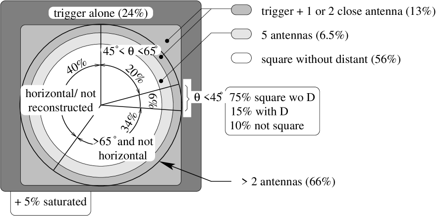
Figure 15: Sketch of the selection cuts used to find the EAS candidates and the corresponding distributions of the event topologies.

The best performance was reached using the restricted band (24–82 MHz) with a low trigger threshold (2 mV). The necessary conditions for satisfactory operation were satisfied only during a few nights (see section 3.3). A careful study of these runs was undertaken and the events were classified using several criteria. The resulting distributions are presented in Fig. 15. It turns out that only 3% of the 3.$10^{3}$ events meet the combined criterion “square & not Distant & $\theta\leq 45^{\circ}$”.

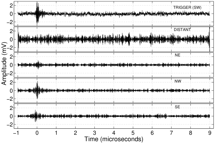
Figure 16: Air shower candidate signals after filtering in the 33–65 MHz band for the event fulfilling all our criteria. The reconstructed direction is $\theta=41^{\circ}$ and $\phi=161^{\circ}$.

The next step in the selection process was to remove any event containing something “suspicious” such as multiple transient pulses within the 10 $\mu$s data record, long duration transient signals ($>1~{}\mu$s) or pulses coming from almost the same location in the sky occurring each day around the same time. This was done on an event-by-event basis. Finally after this very severe scrutiny of candidates, only one event from this data subset appears as a possible EAS candidate (see Fig. 16). This result would seem to be compatible with the cosmic ray flux for energies $\geq 10^{17}$ eV which is $0.2/$km${}^{2}/$hour$/$sr; taking the solid angle corresponding to $\theta\leq 45^{\circ}$ and a surface of collection in the range $0.01-0.1$ km² leads to counting rates from one per 10 days up to one per day. Only further data taking under our best sensitivity conditions together with coincident information from particle detectors will provide us with a better understanding of the acceptance of our device and lead to the appropriate criteria for EAS identification with a self-triggering radio setup.

5.6 Waveform restoration

Waveform information cannot be recovered from the frequency-filtered data, but knowledge of the waveform is mandatory for a complete physical analysis which could contribute to the characterization of the primary cosmic ray. The present section is devoted to discussing possible processing tools able to recover the pulse shape from the raw data.

A typical signal and the radio noise spectrum are shown in Fig. 10 and Fig. 6 respectively. In principle, after transient detection, signal recovery could be achieved by eliminating the various transmitter lines from the frequency spectrum. A simple way to do this is to make a direct subtraction of a noise spectrum derived from the “noise window” from the equivalent “noise+signal” spectrum obtained from the “signal window” (see section 5.2). It was found that this gives poor results due to the strong variability of AM transmitter amplitudes in the 6–25 MHz frequency range. Only signals in the FM band show amplitude stability during the 10 $\mu$s time window. A second difficulty with the strong AM frequency components inherent to the time-bounded nature of data is the leakage phenomenon [26] illustrated in Fig. 17. It can be considerably reduced by performing amplitude limiting on the strongest components above an appropriate threshold [7]. This threshold value is not constant, because reception conditions can vary from one event to another. Taking advantage of the great stability of FM transmitter amplitudes in the 10 $\mu$s record, the amplitude limiting threshold was set at a quarter of the peak value in the FM band. This simple shrinkage method gives excellent results for reducing the leakage phenomenon.

However, though a strong transient could possibly be made visible with this technique, its shape is always modified by AM and FM transmitter residuals. In order to clean the signal, a subsequent processing step is necessary. One possibility is to extract the waveform characteristics from the measured frequency spectrum assuming a simple analytical expression for the pulse shape.

As noted in section 2, the analytical expression of the pulse given by Eq. 2 can be simplified for this purpose. For vertical air showers with small impact parameters, those which give rise to the largest radio signals, $\tau_{2}$ is expected to be much greater than $\tau_{1}$. Furthermore, since the frequency band 24–82 MHz lies above $1/(2\pi\tau_{1})$, the $\tau_{2}$ term gives only a negligible contribution to the Fourier transform in this band and it is neglected. The modulus of the Fourier transform vs frequency $\nu$ then can be written

$$|S(\nu)|=\frac{Ae^{2}\tau_{1}}{2}\frac{1}{(1+4\pi^{2}\nu^{2}\tau_{1}^{2})^{3/2}}$$ (3)

A least squares fit of the spectrum using this expression provides values for $\tau_{1}$ (in ns) and for the amplitude factor A (in volts), thus determining the shape of $S(\nu)$ at all frequencies.

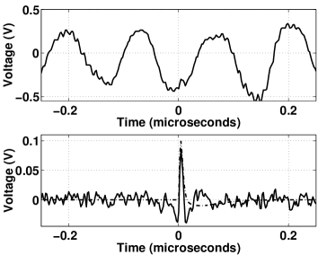
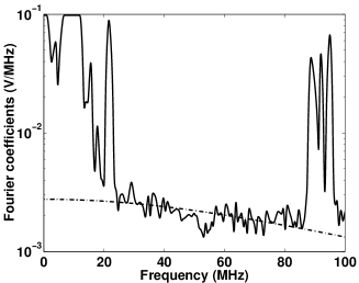
Figure 18: Illustration of signal shape recovery by spectrum fitting. Top left: simulated signal, made up of a typical recorded noise sequence and a pulse added at 0 ns. Bottom left: reconstructed signal in the time domain. The pulse is made visible, though its shape is slightly modified with respect to the simulated one (dash-dotted line). Right: envelope of the Fourier transform modulus (solid line) together with its fit in the 24–82 MHz band (dash-dotted line) after amplitude limiting of the coefficients in the AM transmitter band.

As an example, Fig. 18 illustrates the whole process applied to a simulated signal made up of a typical noise record from one antenna, to which has been added a transient beginning at 0 ns whose shape is given by formula 2. For the full-band configuration the signal is recovered reasonably well for a minimum pulse amplitude of 50 mV and $\tau_{1}\geq 2$ ns. At the moment, the limitation in using this technique experimentally is set principally by our poor ADC resolution. Considering electronic and antenna gains, this sets a lower limit on the peak electric field value of 1.4 mV/m. The method can be used on data from the restricted band for $A\geq$5 mV and $\tau_{1}=2-8$ ns.

This process was applied to the EAS candidate signal of Fig. 16, and gave peak amplitudes A and rise-times $\tau_{1}$ of 16 mV and 4.0 ns, 16 mV and 7.7 ns, and 13 mV and 3.6 ns for the NE, NW and SE antennas respectively. Considering the overall gain factor of the reception chain, the electric field that triggered had a peak value of about 0.4 mV/m.

6 Coincidence measurements

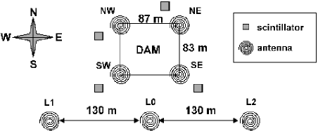
Figure 19: CODALEMA setup for the second phase. The particle detector acts as a trigger with a fourfold coincidence requirement.

In order to investigate possible correlations between measured radio transients and air showers, four stations of particle detectors acting as a trigger have been added. This new setup, including a new antenna configuration, is shown in Fig. 19. It uses seven log-periodic antennas with their electronics (see section 3.3). To get enough sensitivity with our ADCs, all the antenna signals are band pass filtered (24-82 MHz). In this configuration, all the antennas are treated identically.

6.1 Particle detectors

The trigger corresponds to a fourfold coincidence within 600 ns from the particle detectors. These were originally designed as a prototype detector element for the Auger array, consisting of four plastic scintillator modules [27]. Each 2.3 m² module (station) has two layers of acrylic scintillator, read out by a single photomultiplier placed at the center of each sheet. The photomultipliers have copper housings providing electromagnetic shielding. The signals from the upper layers of the four stations are digitized (8-bit ADC, 100 MHz sampling frequency, 10 ${\mu}$s recording time).

A station produces a signal when a coincidence between the two layers is obtained within a 60 ns time interval. This results in a counting rate of around 200 Hz. The rate of the fourfold coincidence of the four stations is about 0.7 events per minute, corresponding almost entirely to air shower events. The four stations are located close to the corners of the DAM array, and in this configuration the particle detectors delimit an active area of roughly $7\times 10^{3}$ m². Using arrival times from the digitized PMT signals, it is possible to determine the direction of the shower by triangulation with a plane fit (same procedure as section 5.3). From the arrival direction distribution, a value of $16\times 10^{3}$ m${}^{2}\times$sr is obtained for the acceptance, which corresponds to an energy threshold of about $1\times 10^{15}$ eV.

6.2 Event analysis

For each fourfold coincidence from the particle detectors, the seven antenna signals are recorded. Due to the relatively low energy threshold of the trigger system, only a small fraction of these air shower events is expected to be accompanied by significant radio signals.

To identify these events, an offline analysis (see section 5) is made. When at least 3 antennas are flagged it becomes possible to apply a triangulation procedure and the event is declared to be a radio candidate if the arrival direction obtained is above the horizon.

The counting rates are the following: 1 event per hour for a single antenna-trigger coincidence, 1 event every 2 hours for a three-fold antennas-trigger coincidence. This indicates that the energy threshold for radio detection is substantially higher than that of the particle array and also that the antennas do not regularly pick up electrical signals related to particle detector activity. Of course, in the 2 $\mu$s window where the search is conducted, a radio transient can occur which is not associated with the air shower. Being uncorrelated, such events should have a uniform arrival time distribution. The next step in the analysis was therefore to study the arrival time distribution of radio signals.

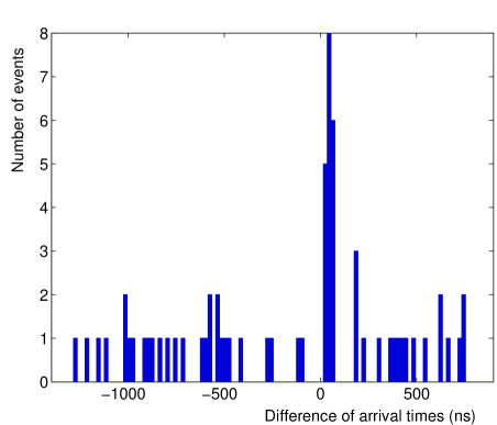
Figure 20: Time delay between the radio plane front and the particle plane front

For radio events that originate from air showers (and possibly from scintillator activity), the radio-particle correlation should manifest itself as a peak in the antenna arrival time distribution, the time reference being furnished by the particle trigger. The width of the raw distribution is primarily determined by the shower arrival direction variation and thus depends on the antenna locations with respect to the particle detectors. For a vertical shower, detectors and antennas will be hit essentially at the same time, neglecting small delays related to the curvature and width of the shower front or small differences between the electromagnetic wave and shower particle propagation times. On the other hand, in the extreme case of a horizontal event coming from the SW direction, the L1 antenna (see Fig. 19) can receive a signal 0.7 $\mu$s before the scintillator located at the NE corner of the DAM array. The time of passage of the radio wavefront through a reference point is compared to the particle front time extracted from the scintillator signals. This time delay distribution is shown in Fig. 20. The data correspond to 59.9 acquisition days and 70 antenna events. A very sharp peak (a few tens of nanoseconds) is obtained showing an unambiguous correlation between certain radio events and the particle triggers. This peak is not exactly centered on zero, the mean value being about 40 ns. The systematic error on these time differences, due to inaccuracies in determining signal times has been estimated to be around 20 ns. The delay between the electric field and particle shower times could be measured with our apparatus, though more thorough studies and higher statistics will be necessary. As expected, there is also a uniform distribution in the 2 $\mu$s window corresponding to accidentals.

A similar arrival time correlation would also have been obtained if the signal on each antenna had been directly induced by a nearby particle detector. However in the present configuration, such an effect can be excluded since three of the seven antennas, which detect signals comparable to those from the other antennas, are not located close to particle detectors. Moreover, it has been verified that no correlation exists between high photomultiplier signal amplitude and the presence of antenna signals.

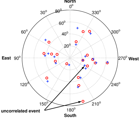
Figure 21: Event arrival directions. The circles indicate directions reconstructed from antenna signals whereas the crosses correspond to directions given by the scintillators. Except for the marked event, each circle is associated with the nearest cross.

Finally, if the time-correlated events correspond to extensive air showers, they must also have correlated arrival directions. Fig. 21 shows, for the 19 events located in the main peak of Fig. 20, the arrival directions reconstructed from both scintillator and antenna data. Except for one event, each antenna direction is associated with the nearest scintillator value. The distribution of the angle between the two reconstructed directions is as expected, i.e., a gaussian centered on zero multiplied by a sine function coming from the solid angle factor. The standard deviation of the corresponding gaussian is about 4 degrees. The one event with a much bigger angular difference is certainly an accidental. The arrival direction given by the antennas is close to the horizon, which is typical of events from radio interference due to human activity. Moreover, the presence of one chance event in the peak is compatible with the observed uniform distribution in the 2 $\mu$s window.

These results strongly support the claim that electric field transients generated by extensive air showers have been measured with CODALEMA, and that the incident direction of the primary cosmic ray can be reconstructed from the arrival times of radio signals.

For the 18 EAS events of Fig. 21 the antenna multiplicity varies from 3 to 7 and the electric field amplitude of the filtered signals goes up to $1.2$ mV$/$m. This signal level corresponds to typical values expected for air shower energies in the $10^{17}$ eV range [4].

In order to obtain a rough estimate for the energy threshold of the present experimental setup, we suppose that the acceptance is the same for the two types of detectors (i.e. $16\times 10^{3}$ m${}^{2}\times$sr). The observed event rate then leads to an approximate energy threshold of $5\times 10^{16}$ eV, using the $\frac{1}{E^{2}}$ power law of the integral cosmic ray flux.

7 Conclusion

The CODALEMA experiment at the Nançay Radio Observatory in central France has shown that this site offers a very good electromagnetic environment for the observation of transient signals with broadband frequency characteristics. Investigation covering a wide frequency span conjugated with numerical filtering and event-by-event noise estimates are the main features which have been implemented in the transient identification procedure.

Convincing evidence has been given for the observation of radio signals associated with extensive air showers by CODALEMA using the coincidence measurements. The originality of this method lies in the possibility of our antenna array to work in a self triggering mode. In particular, we have shown that our antenna array and analysis methods can be used successfully to produce time values and topological information to reconstruct the arrival direction and event waveform. The present results clearly demonstrate the interest of a complete re-investigation of the radio detection method proposed by Aska’ryan in the 1960’s when the performance of the computing and electronics equipment then available was insufficient to identify clearly transient signals from EAS and to discriminate against background.

Improvements in the experimental setup that are in progress include, firstly, additional scintillators to be installed at Nançay to make possible the determination of the shower energy and core position. Two antennas will also be added on each side of the existing W-E line, thereby increasing its length to 600 m providing better sampling of the radio shower signal extension. In a second step, the sensitivity of the array will be increased by the use of 12-bit encoding. This will allow us to record the full 1-100 MHz frequency band and thus to infer shower parameters from the full signal shape. Shower parameters could then be inferred from the signal shape. A dedicated processing tool is being built both for detection and waveform recovery.

In a subsequent upgrade, it is planned to increase the antenna area by the installation of dipole antennas equipped with active front-end electronics. This front-end will use a dedicated ASIC amplifier (gain 35 dB, 1 MHz - 200 MHz bandwidth, $1.3~{}\mathrm{nV/\sqrt{Hz}}$) currently under test. Furthermore, future antennas will be self-triggered and self-time-tagged, coincident events being recognized offline.

The latter point is part of current investigations concerning the feasibility of adding radio detection techniques to an existing surface detector such as the Pierre Auger Observatory. The radio signals should provide complementary information about the longitudinal development of the shower, as well as the ability to lower the energy threshold (depending on the antenna array extension).

Considering that radio detection is expected to offer several specific advantages such as a high duty cycle and a large sensitive volume at moderate cost, this method opens up new prospects for supplementing existing large hybrid detection arrays such as the Pierre Auger Observatory in view of elucidating the enigma surrounding the origin of the highest energy cosmic rays.

Table 1: Electronic sensitivity for the different operating configurations used in the experiment. The last row gives the antenna-related electric field sensitivity.

	Trigger Band	Full Band	Restricted band
	33–65 MHz	1–100 MHz	24–82 MHz
ADC dynamic	$\pm$ 8 mV	$\pm$ 1200 mV	$\pm$80 mV
ADC resolution	0.0625 mV/bit	9.375 mV/bit	0.625 mV/bit
Sensitivity at 50MHz	2 $\mu$V/m/bit	300 $\mu$V/m/bit	20 $\mu$V/m/bit

Figure 2: Pulse waveform (left) and corresponding Fourier transform $|S(\nu)|$ (right) obtained from Eq. (2) using the parameters $\tau_{1}=2$ ns, $A=1$ and $\tau_{2}=20$ ns.

Figure 6: Average Fourier transform $|S(\nu)|$ of the background voltage. The correspondence with the power spectral density in a $50~{}\Omega$ load impedance is shown on the right scale. This spectrum has been obtained by averaging power spectral densities of 900 random events recorded with a sampling frequency of 500 MHz during 10 ${\mu}$s every 10 s. A zoom covering the 0–10 MHz band is presented in the inset.

Figure 17: Mean direct Fourier transform of 900 10 $\mu$s noise snapshots measured at Nançay as a function of the frequency. The inset presents a zoom of the curve for frequencies below 10MHz. The leakage phenomenon is clearly visible in the shape of the spectrum (to be compared with the power spectral density presented in Fig. 6).

References

- [1] Auger Collaboration, Pierre Auger Project Design Report (2nd Edition, Nov. 1996, rev. Mar. 1997) Fermilab, 1997 (available from http://www.auger.org); J.W. Cronin, Rev. Mod. Phys. 71, S165 (1999).
- [2] G.A. Askar’yan, Soviet Physics J.E.T.P., 14 (1962) 441.
- [3] P. Bhattacharjee, G. Sigl, Phys. Rep. 327 (2000) 109.
- [4] H.R. Allan, in: Progress in elementary particle and cosmic ray physics, ed. by J.G. Wilson and S.A. Wouthuysen (North Holland, 1971), p. 169.
- [5] N. Hayashida et al., Phys. Rev. Lett. 73 (1994) 3491. M. Takeda et al., Phys. Rev . Lett. 81 (1998) 1163.
- [6] D.J. Bird et al., Phys. Rev. Lett. 71 (1993) 3401, and Astrophys. J. 441 (1995) 144.
- [7] K. Green, J.L. Rosner, D.A. Suprun, J.F. Wilkerson, Nucl. Instrum. Meth. A498 (2003) 256.
- [8] A. Horneffer, H. Falcke, A. Haungs, K.H. Kampert, G.W. Kant, H. Schieler, proceedings of the 28th International Cosmic Ray Conferences (ICRC 2003), Tsukuba, Japan, 31 Jul - 7 Aug 2003 (to be published); H. Falcke, P. Gorham, Astropart. Phys. 19 (2003) 477.
- [9] http://www.lofar.org
- [10] A. Badea et al., to appear in the proceedings of the 5th Cosmic Ray International Seminar: GZK and Surroundings (CRIS 2004, Catania, Italy, 2004), astro-ph/0409319.
- [11] O.Ravel, R.Dallier, L.Denis, T.Gousset, F.Haddad, P.Lautridou, A.Lecacheux, E.Morteau, C.Rosolen, C.Roy, Proceedings of the 8th Pisa Meeting on Advanced Detectors “Frontier Detectors for Frontier Physics”, Nucl. Instr. Meth. A518 (2004) 213.
- [12] R.Dallier, L.Denis, T.Gousset, F.Haddad, P.Lautridou, A.Lecacheux, E.Morteau, O.Ravel, C.Rosolen, C.Roy, SF2A 2003 Scientific Highlights, ed F. Combes et al. (EDP Sciences, 2003).
- [13] A. Belletoile, D.Ardouin, D. Charrier, R.Dallier, L.Denis, P. Eschstruth, T.Gousset, F.Haddad, J. Lamblin, P.Lautridou, A.Lecacheux, D. Monnier-Ragaigne, A. Rahmani, O.Ravel, SF2A 2004 Scientific Highlights, ed F. Combes et al. (EDP Sciences, 2004), astro-ph/0409039 (2004).
- [14] D. Saltzberg, P. Gorham, D. Walz, C. Field, R. Iverson, A. Odian, G. Resch, P. Schoessow, D. Williams, Phys. Rev. Lett. 86 (2001) 2802.
- [15] J.A. Adams et al., Proceedings of the 4th Tropical Workshop on Particle Physics and Cosmology: Neutrinos, Flavor Physics and Precision Cosmology, Cairns, Queensland, Australia, 9-13 Jun 2003, AIP Conf.Proc.689:3–15,2003.
- [16] P.W. Gorham, K.M. Liewer, C.J. Naudet, Proceedings 26th International Cosmic Ray Conference, Salt Lake City, Utah, 17–25 Aug 1999, vol. 2* 479–482, astro-ph/9906504.
- [17] F.D. Kahn, I. Lerche, Proc. Roy. Soc. A 289 (1966) 206.
- [18] T. Huege, H. Falcke, Astronomy & Astrophysics, 412 (2003) 19; T. Huege, H. Falcke, astro-ph/0409223.
- [19] J.D. Jackson, “Classical Electrodynamics” (Wiley, New York, 1975).
- [20] T. Gousset, O. Ravel, and C. Roy, Astropart. Phys., 22 (2004) 103.
- [21] D. Ardouin, A. Belletoile, D. Charrier, R. Dallier, L. Denis, P. Eschstruth, T. Gousset, F. Haddad, J. Lamblin, P. Lautridou, A. Lecacheux, D. Monnier-Ragaigne, A. Rahmani, O. Ravel, Proceedings of the 19th European Cosmic Ray Symposium, Florence, 2004, astro-ph/0412211.
- [22] D.A. Suprun, P.W. Gorham and J.L. Rosner, Astropart. Phys. 20 (2003) 157.
- [23] http://www.obs-nancay.fr/html_fr/decametr.htm
- [24] J. Lamblin , O. Ravel and C. Medina, internal report SUBATECH 03/2005.
- [25] J.D. Kraus, “Antennas” (McGrawHill, 1988).
- [26] W.H. Press, S.A. J.D. Teukolsky, W.T. Vetterling, B.P. Flannery, “Numerical recipes in C” (Cambridge University Press, 1992).
- [27] M. Boratav, J.W. Cronin, B. Dudelzak, P. Eschstruth, P. Roy, V. Sahakian and Z. Strachman, The AUGER Project: First Results from the Orsay Prototype Station, Proceedings of the 24th ICRC, Rome, 954,(1995).