Chandra HETGS Multi-phase Spectroscopy of the Young Magnetic O Star $\theta^{1}$ Orionis C

Abstract

We report on four Chandra grating observations of the oblique magnetic rotator $\theta^{1}$ Ori C (O5.5 V) covering a wide range of viewing angles with respect to the star’s 1060 G dipole magnetic field. We employ line-width and centroid analyses to study the dynamics of the X-ray emitting plasma in the circumstellar environment, as well as line-ratio diagnostics to constrain the spatial location, and global spectral modeling to constrain the temperature distribution and abundances of the very hot plasma. We investigate these diagnostics as a function of viewing angle and analyze them in conjunction with new MHD simulations of the magnetically channeled wind shock mechanism on $\theta^{1}$ Ori C. This model fits all the data surprisingly well, predicting the temperature, luminosity, and occultation of the X-ray emitting plasma with rotation phase.

1 Introduction

$\theta^{1}$ Ori C, the brightest star in the Trapezium and the primary source of ionization of the Orion Nebula, is the only O star with a measured magnetic field (Donati et al., 2002). This hot star is an unusually strong and hard X-ray source (Yamauchi & Koyama, 1993; Yamauchi et al., 1996; Schulz et al., 2000), with its X-ray flux modulated on the star’s 15-day rotation period (Gagné et al., 1997). Hard, time-variable X-ray emission is not expected from O stars because they do not possess an outer convective envelope to drive a solar-type magnetic dynamo.

Rather, Donati et al. (2002)’s detection of a variable longitudinal magnetic field confirms the basic picture of an oblique magnetic rotator with a dipolar surface field strength, $B\approx 1060$ G. As such, $\theta^{1}$ Ori C, with its relatively strong ($\dot{M}\approx 4\times 10^{-7}$ $\mathrm{M}_{\sun}~{}\mathrm{yr}^{-1}$) radiation-driven wind, may be the prototype of a new class of stellar X-ray source: a young, hot star in which a hybrid magnetic-wind mechanism generates strong and hard, modulated X-ray emission.

Building on the work of Shore & Brown (1990) for Ap/Bp stars, Babel & Montmerle (1997a, b) first described quantitatively the mechanism whereby a radiation-driven wind in the presence of a strong, large-scale dipole magnetic field can be channeled along the magnetic field lines. In this Magnetically Channeled Wind Shock (MCWS) model, flows from the two hemispheres meet at the magnetic equator, potentially at high velocity. This head-on collision between fast wind streams can lead to very high ($T\gg 10^{7}$ K) shock temperatures, much higher than those seen in observations of normal O stars (e.g., $\zeta$ Pup; Hillier et al., 1993). X-ray production in O-type supergiants is attributed to the line-force instability wind shock model (Owocki, Castor, & Rybicki, 1988; Feldmeier, Puls, & Pauldrach, 1997), in which shocks form from interactions between wind streams that are flowing radially away from the star at moderately different speeds.

What makes the MCWS shocks more efficient than instability-driven wind shocks is the velocity contrast experienced in the shocks. The magnetically-channeled wind streams collide with the cool, dense, nearly stationary, post-shock plasma at the magnetic equator. The rapid deceleration of the wind plasma, and the consequent conversion of kinetic energy into heat, causes the strong, hard shocks seen in the MCWS model. This leads to high levels of X-ray emission since a large fraction of the wind kinetic energy is converted into shock heating. In the absence of a strong magnetic field, O-star winds do not produce a fast wind running into stationary plasma; the shocks correspondingly lead to lower shock temperatures and lower luminosity.

This picture of a magnetosphere filled with plasma and corotating with the star, is similar to the picture that has been applied to magnetic Ap/Bp stars (Shore & Brown, 1990; Shore et al., 1990; Smith & Groote, 2001). Indeed Babel & Montmerle’s first paper on the subject was an application to the Ap star IQ Aur (Babel & Montmerle, 1997a). However, a major difference between the model’s application to Ap/Bp stars and to young O stars is that the winds of O stars are significantly stronger, representing a non-negligible fraction of the star’s energy and momentum output. This hybrid magnetic wind model thus is more than a means of explaining the geometry of circumstellar material, but also can potentially explain the intense hard X-ray emission from young, magnetized hot stars (three orders of magnitude greater for $\theta^{1}$ Ori C than for IQ Aur). As has been pointed out in the context of the magnetic Ap/Bp stars, if the dipole field is tilted with respect to the rotation axis, then the rotational modulation of our viewing angle of the magnetic pole and its effect on observed flux levels and line profiles provides a important diagnostic tool. We exploit this fact by making several Chandra observations of $\theta^{1}$ Ori C at different rotational phases, in order to study the dynamics and geometry of the hot, X-ray emitting plasma in the circumstellar environment of this young, magnetized O star and thus to assess the mechanism responsible for generating the unusual levels of X-ray emission in $\theta^{1}$ Ori C.

The time independent nature of the original Babel & Montmerle model leads to a steady-state configuration in which a post-shock “cooling disc” forms at the magnetic equator. In their model, this disk is essentially an infinite mass sink. This has an effect on the assumed X-ray absorption properties of the disk and it also affects the steady state spatial, temperature, and velocity distribution of the hot, X-ray emitting plasma, thus affecting the quantitative predictions of observables in unphysical ways. Babel & Montmerle (1997b) further assume a rigid magnetic geometry within the magnetosphere, thereby imposing a pre-specified trajectory to the wind streams; namely they are forced to flow everywhere along the local dipole field direction. In reality, if the wind kinetic energy is large enough, the magnetic field should be distorted. In the extreme case of a field that is (locally) weak compared to the wind kinetic energy, the initially closed field lines will get ripped open and the flow (and field lines) will be radial, and the focusing of the wind flow toward the equator and the associated shock heating will be minimized. Babel & Montmerle (1997b) recognized these limitations and speculated about the effects of relaxing the strong-field and steady-state assumptions (see also Donati et al., 2002).

To explore these effects, ud-Doula & Owocki (2002) performed magneto-hydrodynamic (MHD) simulations of radiation-driven winds in the presence of a magnetic field. Their results confirmed the basic paradigm of the Babel & Montemerle model wherein a magnetic field channels the wind material towards the magnetic equator where it shocks and cools. If the field is strong enough it can even confine the wind. The overall degree of such a confinement can be determined by a single dimensionless parameter, $\eta_{\star}$, which represents the ratio of the magnetic energy density to the wind kinetic energy density.

$$\eta_{\star}=\frac{B^{2}_{\rm eq}R^{2}_{\star}}{\dot{M}v_{\infty}},$$ (1)

where $B_{\rm eq}$ is the equatorial dipole magnetic intensity at the stellar surface, $R_{\star}$ is the stellar radius, $\dot{M}$ is the mass-loss rate, and $v_{\infty}$ is the terminal wind speed. For $\eta_{\star}\lesssim 1$, the field is relatively weak and the wind dominates over the magnetic field by ripping the field lines into a nearly radial configuration. Nonetheless, the field still manages to divert some material towards the magnetic equator leading to a noticeable density enhancement. Because the magnetic field energy density falls off significantly faster than the wind kinetic energy density, at large radii, the wind always dominates over the field, even for $\eta_{\star}\gg 1$. The MHD simulations reveal some phenomena not predicted by the static Babel & Montmerle model. Above the closed magnetosphere near the magnetic equator where the field lines start to open up, the magnetically channeled wind still has a large latitudinal velocity component, leading to strong shocks.

The simulations show shock-heated wind plasma above and below the magnetic equatorial plane where it cools and then falls along closed magnetic field lines. This cool, dense, post-shock plasma forms an unstable disk. Mass in the disk builds up until it can no longer be supported by magnetic tension, at which time it falls back down onto the photosphere. The star’s rotation and the obliquity of the magnetic axis to the rotation axis lead to periodic occultation of some of the X-ray emitting plasma. All of these phenomena should lead to observable, viewing-angle dependent diagnostics: temperature distribution, Doppler line broadening, line shifts, and absorption.

The initial 2D MHD simulations performed by ud-Doula & Owocki (2002) were isothermal, and the shock strength and associated heating were estimated based on the shock-jump velocities seen in the MHD output. For the analysis of the Chandra HETGS spectra discussed in this paper, however, new simulations were performed that include adiabatic cooling and radiative cooling as well as shock heating in the MHD code’s energy equation. In this way, we make detailed, quantitative predictions of plasma temperature and hence X-ray emission for comparison with the data. Furthermore, the changes in gas pressure associated with the inclusion of heating and cooling has the potential to affect the dynamics and thus the shock physics and geometry of the magnetosphere. We thus present the most physically realistic modeling to date of X-ray production in the context of the MCWS model.

In this paper we present two new observations of $\theta^{1}$ Ori C taken with the HETGS aboard Chandra, which we analyze in conjunction with two GTO observations, previously published by Schulz et al. (2000, 2003). These four observations provide good coverage of the rotational phase and hence sample a broad range of viewing angles with respect to the magnetosphere. We apply several spectral diagnostics, including line-width analysis for plasma dynamics, line-ratio analysis for distance from the photosphere, differential emission measure for the plasma temperature distribution, and overall X-ray spectral variability for the degree of occultation and absorption, to these four data sets. In this way, we characterize the plasma properties and their variation with phase, or viewing angle, allowing us to compare these results to the output of MHD simulations and assess the applicability of the MCWS model to this star.

In §2 we describe the data and our reduction and analysis procedure. In §3 we discuss the properties of $\theta^{1}$ Ori C. §4 we describe the MHD modeling and associated diagnostic synthesis. In §5 we report on the results of spectral diagnostics and their variation with phase. In §6 we discuss the points of agreement and disagreement between the modeling and the data, critically assessing the spatial distribution of the shock-heated plasma and its physical properties in light of the observational constraints and the modeling. We conclude with an assessment of the applicability of hybrid magnetic-wind models to $\theta^{1}$ Ori C in §7.

2 Chandra Observations and Data Analysis

The Chandra X-ray Observatory observed the Trapezium with the High Energy Transmission Grating (HETG) spectrometer twice during Cycle 1 and twice during Cycle 3. The Orion Nebula Cluster was also observed repeatedly during Cycle 4 with the ACIS-I camera with no gratings. Table 1 lists each observation’s Sequence Number, Observation ID (OBSID), UT Start and End Date, exposure time (in kiloseconds), average phase, and average viewing angle (in degrees). The phase was calculated using a period of 15.422 days and a zero-point MJD=48832.5 (Stahl et al., 1996). Assuming a centered oblique magnetic rotator geometry (see Figure 1), the viewing angle $\alpha$ between the line of sight and the magnetic pole is specified by:

$$\cos\alpha=\sin\beta\cos\phi\sin i+\cos\beta\cos i,$$ (2)

where $\beta=42\arcdeg$ is the obliquity (the angle between the rotational and magnetic axes), $i=45\arcdeg$ is the inclination angle, and $\phi$ is the rotational phase of the observation (in degrees). In Fig. 1, the arrows at each viewing angle point to Earth. As the star rotates, the viewing angle varies from $\alpha\approx 3\arcdeg$ (nearly pole-on) at phase $\phi=0.0$ to $\alpha\approx 87\arcdeg$ (nearly edge-on) at phase $\phi=0.5$. The four grating observations were obtained at $\alpha\approx 4\arcdeg,40\arcdeg,80\arcdeg$, and $87\arcdeg$, thus spanning the full range of possible viewing angles. An online animation illustrates our view of the magnetosphere as a function of rotational phase.

The Chandra HETG data were taken with the ACIS-S camera in TE-mode. During OBSID 3 and 4, ACIS CCDs S1-S5 were used; S0 was not active. During OBSID 2567 and 2568, ACIS CCDs S0-S5 were used. The data were reduced using standard threads in CIAO version 2.2.1 using CALDB version 2.26. Events with standard ASCA grades 0, 2, 3, 4, and 6 were retained. The data for CCD S4 were destreaked because of a flaw in the serial readout which causes excess charge to be deposited along some rows. The data extraction resulted in four first-order spectra for each observation: positive and negative first-order spectra for both the medium-energy grating (MEG) and high-energy grating (HEG).

A grating Auxiliary Response File (ARF) was calculated for each grating spectrum. The negative and positive first order spectra were then coadded for each observation using the CIAO program ADD_GRATING_ORDERS. The four sets of MEG and HEG spectra are shown in the top four panels of Figures 2 and 3. The first-order MEG spectra from each of the four observations were then co-added to create the spectrum in the bottom panel of Fig. 2. The co-added HEG spectrum is shown in the bottom panel of Fig. 3. The MEG gratings have lower dispersion than the HEG gratings. However, the MEG is more efficient than the HEG above 3.5 Å. The added spectral resolution of the HEG is useful for resolving line profiles and resolving lines that may be blended in the MEG spectrum. Because the HEG and MEG wavelength solutions were in excellent agreement, the MEG and HEG spectra were fit together to increase signal-to-noise.

The spectra show very strong line and continuum emission below 10 Å indicating a very hot, optically thin plasma. The relatively low line-to-continuum ratio from 9–12 Å suggests sub-solar Fe abundance. Photons with $\lambda>24$ Å are nearly entirely absorbed by neutral hydrogen, helium and metals in the wind of $\theta^{1}$ Ori C, in the neutral lid of the Orion Nebula and in the line-of-sight ISM.

We analyzed the extracted spectra in several different ways. In §5 we discuss the diagnostics that we bring to bear on the determination of the properties of the hot plasma, but first we describe our data analysis procedures. Our first goal was to determine centroid wavelengths, intensities and non-instrumental line widths for the eighty or so brightest emission lines. Our second goal was to determine the basic physical properties of the X-ray emitting plasma.

2.1 Global Spectral Fits

In order to determine the temperatures, emission measures, and abundances of the emitting plasma and the column density of the overlying gas, we fit the HEG/MEG spectra using the ISIS software package. We obtained acceptable fits to the 1.8–23 Å HEG and MEG spectra using a two-temperature variable-abundance APED emission model with photo-electric absorption from neutral ISM gas (Morrison & McCammon, 1983). The free parameters were the column density, the two temperatures, the two normalizations, the redshift, the turbulent velocity, and the abundances of O, Ne, Mg, Si, S, Ar, Ca and Fe.

We note that a number of emission-measure profiles EM(T) can be used to fit the spectra, all giving rise to similar results: a dominant temperature component near 30 MK, and a second temperature peak near 8 MK. We chose the simplest model with the fewest free parameters that adequately fit the data: a two-temperature, variable abundance APEC model in ISIS. We also note that with all the thermal emission models we tried, non-solar abundances were needed to correctly fit the emission lines.

As we shall discuss in §5, we find small, but significant, shifts in the line centroids. The ISIS plasma emission model has one advantage compared to those in SHERPA and XSPEC: it explicitly and consistently accounts for thermal, non-thermal, and instrumental line broadening. The width of a line corrected for instrumental broadening is the Doppler velocity, $v_{D}$, as defined by Rybicki & Lightman (1979):

$$v_{D}=\frac{c}{\lambda_{0}}{\Delta\lambda_{D}}=\frac{c}{\lambda_{0}}\frac{{\rm FWHM}}{\sqrt{\ln 16}}={\left(\frac{2kT}{m}+\xi^{2}\right)}^{\frac{1}{2}},$$ (3)

where $v_{\rm th}=\sqrt{\frac{2kT}{m}}$ is the thermal broadening component and $\xi$ is the rms of the turbulent velocities. $\xi$ is used simply as a standard means of parameterizing the component of the line width caused by non-thermal bulk motion (assumed to be Gaussian). As we discuss further in §5, the non-thermal, non-instrumental width parametrized by $\xi$ is probably the result of bulk motion of shock-heated wind plasma, and not, strictly speaking , physical microturbulence as described by Rybicki & Lightman (1979). Note that $v_{D}$ and $\xi$ thus defined are related to $v_{\rm HWHM}$, often used as a velocity-width parameter when broadening is due to a stellar wind, as $v_{\rm HWHM}=0.83v_{D}$.

The spectral anaylsis showed no obvious changes in abundance with phase. The best-fit abundances and $1\sigma$ uncertainties are shown in the “Global Fit” column of Table 5. These abundances were then fixed for the fits at each rotational phase. Those best-fit parameters and $1\sigma$ uncertainties are shown in Table 6. The most notable result of the global fitting is that most of the plasma is at $T\approx 30$ MK and that the temperatures do not vary significantly with phase. The phase-to-phase spectral variations seen in Figs. 2 and 3 appear to be caused by changes in visible emission measure. One disadvantage of this type of global fitting is that the thermal emission models currently in ISIS, SHERPA and XSPEC do not account for the effects of high density and/or UV radiation. For this, we model the individual line complexes (see §5.2).

2.2 Line Profile Analysis

SHERPA, the CIAO spectral fitting program, was used to fit the 24 strongest line complexes of O, Ne, Mg, Si, S, Ar, Ca, and Fe in the 1.75 to 23 Å range. In the 3–13 Å region, the HEG and MEG spectra were simultaneously fit for each complex. Below 3 Å the MEG spectra have low S/N and only the HEG spectra were used. Above 13 Å the HEG spectra have low S/N and only the MEG spectra were used. Because each line complex typically contains one to eight relatively bright lines, multiple Gaussian components were used to model the brightest lines in a complex (as estimated by their relative intensities at 30 MK in APED). Emission from continua and very faint lines across each complex was modeled simply as an additive constant. We note, e.g., that unresolved doublets were modeled as two Gaussians, with the emissivity of the fainter of the pair tied to the emissivity of the brighter. To further minimize the number of free parameters, the centroid wavelengths and widths of all lines in a complex were tied to that of the brightest line in that complex.

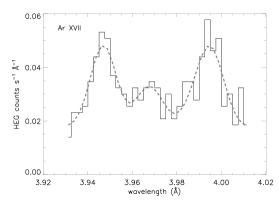
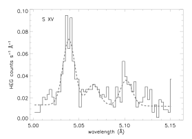
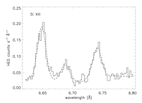
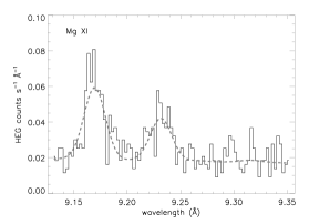
Figure 12: Ar XVII, S XV, Si XIII, and Mg XI He-like line complexes. In each panel, the data (solid histogram) and model (gray dashed line) of the resonance (r), intercombination (i) and forbidden (f) lines are shown. Note that as atomic number increases from $Z=12$ (Mg XI) to $Z=18$ (Ar XVII), the relative strength of the forbidden line to the intercombination line increases. The Si XIII f line is blended with a Mg XII line. The other detected He-like lines were not used for the diagnostic analysis: Ca XIX was too weak and the Fe XXV f and i lines were not resolved.

For example, a typical He-like line complex like Si XIII (see Figure 12c) was modeled with six Gaussians: the Si XIII resonant (singlet), intercombination (doublet), and forbidden (singlet) lines plus the Mg XII resonant doublet. This particular complex had six free parameters: one constant, one line width, one line shift (relative to APED) and three intensities (Si XIII resonance, one Si XIII intercombination, and Si XIII forbidden). In this case, the Mg XII emission was blended with the Si XIII forbidden line. In these cases, blending leads to higher uncertainties in the line parameters. In this example, the Mg XII line was accounted for by tying its flux to the flux of the Si XIII resonance line, scaled by the emissivity ratio of those lines in APED and the Mg/Si ratio from globally fitting the HEG/MEG spectra.

The resulting SHERPA fits are shown in the first nine columns of Table 2. The ion, transition, and rest wavelength $\lambda_{0}$ are from APED. Free parameters have associated $1\sigma$ errors, tied parameters do not. As expected, line and continuum fluxes were approximately 30% higher during OBSID 2567 (viewing angle $\alpha=4\arcdeg$) than during OBSID 2568 ($\alpha=87\arcdeg$), with intermediate fluxes during OBSID 3 and 4.

Because SHERPA does not explicitly account for thermal and non-thermal line broadening, the individual line complexes were fit a second time with ISIS to derive the rms turbulent velocities and abundances. $\xi$ and the relevant abundance parameters for a given line complex were allowed to vary while the emission and absorption parameters (temperatures, normalizations, other abundances, and column density) were frozen. The resulting abundances and $1\sigma$ uncertainties are listed in the “Line Fit” column of Table 5. The Fe abundance was determined from numerous ionization stages in six line complexes. For Fe, $\sigma$ is the standard deviation of these six Fe abundance fits. The individual rms turbulent velocities $\xi$ are listed in the last two columns of Table 2.

Summarizing the results of the spectral fitting, we conclude that some elements (especially Fe) have non-solar abundances, most of the plasma is at a temperature around 30 MK, the lines are resolved but much narrower than the terminal wind velocity, and only the overall emission measure appears to vary significantly with phase.

We note that the zeroth-order ACIS-S point-spread function of $\theta^{1}$ Ori C is substantially broader than nearby point sources and substantially broader than the nominal ACIS PSF. We have taken the best-fit model from ISIS and made MARX simulations of the zeroth-order PSF. The simulations show that the excess broadening in the zeroth-order image is a result of pileup in the ACIS-S CCD. Pixels in the core of the PSF register multiple events occurring within a single 3.2 s readout as a single higher-energy count. In the wings of the PSF, the count rate per pixel is much lower and pileup is reduced. Hence the spatial profile is less peaked than it would be without pileup. Because the count rate per pixel in the first-order lines is much lower than in zeroth order, the lines in the dispersed spectra are not broadened by pileup. We conclude that the measured line velocities are not caused by instrumental effects. Non-intrumental Gaussian line shapes provide adequate fits to the data. Non-Gaussian line shapes, while perhaps present, could only be detected with higher S/N data.

3 Properties of $\theta^{1}$ Ori C

In order to put the results of the spectral fitting and the MHD modeling into a physical context, we must first specify the stellar and wind parameters of $\theta^{1}$ Ori C as well as elaborate on the geometry and distribution of circumstellar matter, as constrained by previous optical and UV measurements. The spectral type of the star is usually taken to be O6 V or O7 V, although its spectral variability was first noted by Conti (1972). Donati et al. (2002) assume a somewhat hot effective temperature, $T_{\rm eff}=45500$ K, which is based on the O5.5 V type used by Howarth & Prinja (1989), which itself is an average of Walborn’s (1981) range of O4-O7. Walborn (1981) showed that lines often used to determine spectral type (He I $\lambda 4471$, He II $\lambda 4542$ and $\lambda 4686$) are highly variable on time scales of about a week, suggesting a period “on the order of a few weeks”. He compared $\theta^{1}$ Ori C’s line-profile variations to those of the magnetic B2 Vp star $\sigma$ Orionis E, even noting then that $\theta^{1}$ Ori C’s X-ray emission, recently discovered with the Einstein Observatory, may be related to its He II $\lambda 4686$ emission.

Based on a series of H$\alpha$ and He II $\lambda 4686$ spectra obtained over many years, Stahl et al. (1993, 1996) and Reiners et al. (2000) have determined that the inclination angle of $\theta^{1}$ Ori C is $i\approx 45\arcdeg$ and the rotational period $P=15.422\pm 0.002$ days. The inclination angle estimate is based on arguments about the symmetry of the light curve and spectral variability as well as plausibility arguments based on the inferred stellar radius. As expected from its long rotation period, $\theta^{1}$ Ori C’s projected rotational velocity is quite low, with Reiners et al. (2000) finding a value of $v\sin i=32\pm 5$ km s^-1 using the O III $\lambda 5592$ line core.

The Zeeman signature measurements of Donati et al. (2002) indicate a strong dipole field, with no strong evidence for higher order field components. The five sets of Stokes parameters indicate a magnetic obliquity $\beta\approx 42\arcdeg$ if $i=45\arcdeg$. These numbers then imply a photospheric polar magnetic field strength of $B_{\mathrm{p}}=1060\pm 90$ G. The obliquity and polar field strength take on modestly different values if the inclination angle is assumed to be as small as $i=25\arcdeg$ or as large as $i=65\arcdeg$.

As a result of these various determinations of stellar properties, we adopt two sets of stellar parameters that likely bracket those of $\theta^{1}$ Ori C. These are listed in Table 3, and are based on the PHOENIX spherical NLTE model atmospheres of Aufdenberg (2001).

The theoretical wind values listed in Table 3 are consistent with the observed values of $\dot{M}=4\times 10^{-7}$ $\mathrm{M}_{\sun}~{}\mathrm{yr}^{-1}$ (Howarth & Prinja, 1989) and $v_{\infty}\approx 2500$ km s^-1 (Stahl et al., 1996). The stellar wind properties, as seen in UV resonance lines, are modulated on the rotation period of the star (Walborn & Nichols, 1994; Reiners et al., 2000), which, when combined with variable H$\alpha$ (Stahl et al., 1996) and the new measurement of the variable magnetic field (Donati et al., 2002), lead to a coherent picture of an oblique magnetic rotator, with circumstellar material channeled along the magnetic equator. This picture is summarized in Fig. 1, which also indicates the viewing angle relative to the magnetic field for our four Chandra observations.

When we see the system in the magnetic equatorial plane, the excess UV wind absorption is greatest. When we see the system magnetic pole on, the UV excess is at its minimum, while the longitudinal magnetic field strength is maximum, as are the X-ray and H$\alpha$ emission (Stahl et al., 1993; Gagné et al., 1997). These results are summarized in Figure 4, where we show fourteen days of data from the 850-ks Chandra Orion Ultra-Deep Project. These data were obtained with the ACIS-I camera with no gratings. Because $\theta^{1}$ Ori C’s count rate far exceeds the readout rate of the ACIS-I CCD, the central pixels of the source suffer from severe pileup. For Fig. 4b, counts were extracted from an annular region in the wings of the PSF where pileup was negligeable As a result, the Chandra light curve does not show the absolute count rate in the ACIS-I instrument. The light curve shows long-term variability induced by rotation and occultation and statistically significant short-term variability that may reflect the dynamic nature of the magnetically channeled wind shocks.

These four different observational results are consistent with this picture provided that the H$\alpha$ emission is produced in the post-shock plasma near the magnetic equatorial plane. Smith & Fullerton (2005) have re-analyzed the 22 high-dispersion IUE spectra of $\theta^{1}$ Ori C and re-interpreted the time-variable UV and optical line profiles in terms of the magnetic geometry of Donati et al. (2002). Smith & Fullerton (2005) find that the C IV and N V lines at phase 0.5 (nearly edge-on) are characterized by high, negative-velocity absorptions and lower, positive-velocity emission, superposed on the baseline P Cygni profile. Similarly, some of the optical Balmer-line and He II emissions appear to be produced by post-shock gas falling back onto to the star. In the following sections, we further constrain and elaborate on this picture by using several different X-ray diagnostics in conjunction with MHD modeling.

We note finally that $\theta^{1}$ Ori C has at least one companion. Weigelt et al. (1999) find a companion at 33 mas via infrared speckle interferometry. Donati et al. (2002) estimate its orbital period to be 8–16 yr and Schertl et al. (2003) estimate its spectral type as B0-A0. This places the companion at 15 AU, too far to significantly interact with the wind or the magnetic field of $\theta^{1}$ Ori C. The amplitude and timescale of the X-ray luminosity variations cannot be caused by colliding-wind emission with the companion, by occultation by the companion, or by the companion itself (Gagné et al., 1997).

4 Magneto-Hydrodynamical Modeling of the Magnetically Channeled Wind of $\theta^{1}$ Ori C

4.1 Basic Formulation

As discussed in the Introduction, we have carried out MHD simulations tailored specifically for the interpretation of the $\theta^{1}$ Ori C X-ray data presented in this paper. Building upon the full MHD models by ud-Doula & Owocki (2002), these simulations are self-consistent in the sense that the magnetic field geometry, which is initially specified as a pure dipole with a polar field strength of 1060 G, is allowed to adjust in response to the dynamical influence of the outflowing wind. As detailed below, a key improvement over the isothermal simulations of ud-Doula & Owocki (2002) is that we now use an explicit energy equation to follow shock heating of material to X-ray emitting temperatures.

The overall wind driving, however, still follows a local CAK/Sobolev approach that suppresses the “line deshadowing instability” for structure on scales near and below the Sobolev length, $l\approx v_{\rm th}r/v\approx 10^{-2}r$, with $r$ the radius and $v$ and $v_{\rm th}$ the flow and thermal speeds (Lucy & Solomon, 1970; MacGregor et al., 1979; Owocki & Rybicki, 1984, 1985). For non-magnetic winds, 1-D simulations using a non-local, non-Sobolev formulation for the line-force (Owocki, Castor, & Rybicki, 1988; Owocki & Puls, 1999; Runacres & Owocki, 2002) show this instability can lead to embedded weak shock structures that might reproduce the soft X-ray emission (Feldmeier, 1995; Feldmeier, Puls, & Pauldrach, 1997) observed in hot stars like $\zeta$ Pup (Waldron & Cassinelli, 2001; Kramer, Cohen, & Owocki, 2003). However, it seems unlikely that such small-scale, weak-shock structures can explain the much harder X-rays oberved from $\theta^{1}$ Ori C. Given, moreover, the much greater computational expense of the non-local line-force computation, especially for the 2D models computed here (Dessart & Owocki, 2003, 2005), we retain the much simpler, CAK/Sobolev form for the line-driving. In the absence of a magnetic field, such an approach just relaxes to the standard, steady-state, spherically symmetric CAK solution. As such, the extensive flow structure, and associated hard X-ray emission, obtained in the MHD models here are a direct consequence of the wind channeling by the assumed magnetic dipole originating from the stellar surface.

Since the circa 15-day rotation period of $\theta^{1}$ Ori C is much longer than the characteristic wind flow time of a fraction of a day, we expect that associated centrifugal and coriolis terms should have limited effect on either the wind dynamics or magnetic field topology. Thus, for simplicity, and to retain the computational efficiency of axisymmetry, the numerical simulations here formally assume no rotation. However, in comparing the resulting X-ray emission to observations, we do account for the rotational modulation arising from the change in observer viewing angle with rotational phase, using the estimated inclination angle $i\approx 45\arcdeg$ between the rotation axis and the observer’s line of sight, and obliquity $\beta\approx 42\arcdeg$.

4.2 Energy Balance with Shock Heating and Radiative Cooling

In order to derive quantitative predictions for the X-ray emission from the strong wind shocks that arise from the magnetic confinement, the simulations here extend the isothermal models of ud-Doula & Owocki (2002) to include now a detailed treatment of the wind energy balance, accounting for both shock heating and radiative cooling. Specifically, the total time derivative ($D/Dt$) of wind internal energy density $e$ (related to the gas pressure $p$ by $e=p/(\gamma-1)=(3/2)p$ for a ratio of specific heats $\gamma=5/3$ appropriate for a monatomic gas) is computed from

$$\rho\,\frac{D(e/\rho)}{Dt}=-\rho\nabla\cdot p+H-C\,,$$ (4)

where $\rho$ is the mass density, and $H$ and $C$ represent volumetric heating and cooling terms. In steady hot-star winds, the flow is kept nearly isothermal at roughly the stellar effective temperature (few $\times 10^{4}$ K) through the near balance between heating by photoionization from the underlying star and cooling by radiative emission (mostly in lines, see, e.g., Drew, 1989). In such steady outflows, both the heating and cooling terms are intrinsically much larger than the adiabatic cooling from the work expansion, as given by the first term on the right-hand-side of the energy equation.

But in variable, structured winds with compressive shocks, this first term can now lead to strong compressive heating, with some material now reaching much higher, X-ray emitting temperatures. Through numerical time integrations of the energy equation, our MHD simulations account directly for this compressive heating near shocks, imposing also a floor value at the photospheric effective temperature to account for the effect of photoionization heating on the relatively cool, expanding regions. In the simulations, the temperature of the far wind is $T=45700$ K, slightly warmer than the O5.5 photosphere (see Table 3).

The shock-heated material is cooled by the radiative loss term, which is taken to follow the standard form for an optically thin plasma,

$$C\,=\,n_{\rm e}\,n_{\rm H}~{}\mathcal{L}(T)\,,$$ (5)

where $n_{\rm e}$ and $n_{\rm H}$ are the numbers densities for electrons and hydrogen atoms, and $T$ is the electron temperature.

A proper radiative cooling calculation must include many different ionic species with all the possible lines (Raymond, Cox & Smith, 1976; MacDonald & Bailey, 1981), with the exact form of the cooling function $\mathcal{L}(T)$ depending on the composition of heavy elements. Detailed calculations for the typical case of solar abundances show that, at low temperatures, the cooling function $\mathcal{L}(T)$ increases approximately monotonically with temperature, reaching a maximum, $\mathcal{L}\approx 3\times 10^{-22}$ erg cm³ s^-1, at $T\approx 2\times 10^{5}$ K (Raymond, Cox & Smith, 1976), where the cooling is dominated by collisional excitation of abundant lithium-like atoms. Above $T\approx 2\times 10^{5}$ K, $\mathcal{L}(T)$ decreases with temperature, except for some prominent bumps at approximately 2 and 8 MK. Above $T\approx 3\times 10^{7}$ K, thermal brehmsstrahlung radiation dominates and the cooling function turns over again, increasing with temperature. In our simulations, we follow the tabulated form of the MacDonald & Bailey (1981) cooling curve based on this solar-abundance recipe.

4.3 Simulations Results for Temperature and Emission Measure

One of the key results of ud-Doula & Owocki (2002) is that the overall degree to which the wind is influenced by the magnetic field depends largely on a single parameter, the magnetic confinement parameter, $\eta_{\star}$, defined by equation 1. For our MHD simulations here of the magnetic wind confinement in $\theta^{1}$ Ori C, we use $\eta_{\star}=7.5$, based on an assumed stellar radius $R_{\star}\approx 9R_{\sun}$ (see Table 3), $B_{\rm eq}=\frac{1}{2}B_{\mathrm{p}}\approx 530$ G (Donati et al., 2002). The simulation produces an average mass-loss rate ${\dot{M}}\approx 4\times 10^{-7}M_{\odot}$ yr^-1 (Howarth & Prinja, 1989), and terminal wind speed $v_{\infty}\approx 1400$ km s^-1. Thus, we anticipate that, at least qualitatively, the simulation results for $\theta^{1}$ Ori C should be similar to the strong magnetic confinement case ($\eta_{\star}=10$) shown in Fig. 9 of ud-Doula & Owocki (2002), allowing however for differences from the inclusion now of a full energy equation instead of the previous assumption of a strictly isothermal outflow.

We note that $\theta^{1}$ Ori C’s observed terminal wind speed derived from IUE high-resolution spectra (Howarth & Prinja, 1989; Prinja et al., 1990; Walborn & Nichols, 1994) varies significantly, with $v_{\infty}\approx 510$ km s^-1 at rotational phase 0.1, when the wind absorption is weak (see top panel of Fig. 4). $\theta^{1}$ Ori C’s wind speed and mass-loss rate are lower than those of other mid-O stars and lower than expected from model atmosphere calculations (see Table 3). In the interpretation of Smith & Fullerton (2005) and Donati et al. (2002), most of the wind is channeled to the magnetic equatorial region. Thus, ${\dot{M}}$ and $v_{\infty}$ are low near X-ray maximum (phase 0.0) when the star is viewed magnetic pole-on. It is also worth noting that Prinja et al. (1990) measure a narrow absortion-line component velocity $v_{\rm NAC}\approx 350$ km s^-1 at phase 0.1, comparable to the Doppler velocity of the X-ray lines discussed in §5. In contrast, Stahl et al. (1996) measure a maximum edge velocity $v_{\rm edge}\approx 2500$ km s^-1. The net result is that the confinement parameter for $\theta^{1}$ Ori C is in the approximate range $5\leq\eta_{\star}\leq 20$. The low terminal wind speed, $v_{\infty}\approx 510$ km s^-1, measured by Prinja et al. (1990) is lower than the escape velocity of $\theta^{1}$ Ori C, $v_{\rm esc}\approx 1000$ km s^-1. Our $\eta_{\star}\approx 7.5$ model produces a $1470$ km s^-1 wind above the magnetic pole.

Starting from an intial time $t=0$ when the dipole magnetic field is suddenly introduced into a smooth, steady, spherically symmetric, CAK wind, our MHD simulation follows the evolution through a total time interval, $t=500$ ks, that is many characteristic wind flow times, $R_{\star}/v_{\infty}\approx 5$ ks. Figure 5 is a snapshot of the spatial distribution of log emission measure per unit volume (upper panel) and log temperature (lower panel) at a time, $t=375$ ks, when material is falling back onto the photosphere along magnetic field lines (solid lines).

After introduction of the field, the wind stretches open the field lines in the outer region. In the inner reqion, the wind is channeled toward the magnetic equator by the closed field lines. Within these closed loops, the flow from opposite hemisphere collides to make strong, X-ray emitting shocks. At early times, the shocks are nearly symmetric about the magnetic equatorial plane, like those predicted in the semi-analytic, fixed-field models of Babel & Montmerle (1997b). 2D movies of $\theta^{1}$ Ori C show the evolution of density, temperature, and wind speed from the initially dipolar configuration.

Fig. 5 shows, however, that the self-consistent, dynamical structure is actually much more complex. This is because once shocked material cools, its support against gravity by the magnetic tension along the convex field lines is inherently unstable, leading to a complex pattern of fall back along the loop lines down to the star. As this infalling material collides with the outflowing wind driven from the base of a given loop line, it forms a spatially complex, time-variable structure, thereby modifying the location and strength of the X-ray emitting shocks. When averaged over time, however, the X-ray emission appears to be symmetric and smooth.

It should be emphasized here that the implied time variability of shock structure and associated X-ray emission in this simulation is made somewhat artificial by the assumed 2-D, axisymmetric nature of the model. From a more realistic 3-D model (even without rotation), we expect the complex infall structure would generally become incoherent between individual loop lines at different azimuths (i.e. at different magnetic longitudes). As such, the azimuthally averaged, X-ray emission in a realistic 3-D model is likely to be quite similar to the time-averaged value in the present model. A reliable determination of the expected residual level of observed X-ray variability in such wind confinement models must await future 3-D simulations that account for the key physical processes setting the lateral coherence scale between loops at different azimuth. But based on the fine scale of magnetic structure in resolved systems like the solar corona, it seems likely that this lateral coherence scale may be quite small, implying then only a low level of residual variability in spatially integrated X-ray spectra.

Overall, we thus see that introduction of the initial dipole magnetic field results in a number of transient discontinuities that quickly die away. The wind in the polar region stretches the magnetic field into a nearly radial configuration and remains quasi-steady and smooth for the rest of the simultion. However, near the equatorial plane where the longitudinal component of the magnetic field, $B_{\theta}$, is large, the wind structure is quite complex and variable. In the closed field region within an Alfvén radius, $R\approx 2R_{\star}$, the field is nearly perpendicular to the magnetic equatorial plane and strong enough to contain the wind. The material from higher latitudes is thus magnetically channeled towards the equator and can reach velocities $v_{\theta}\approx 1000$ km s^-1.

Such high speeds lead to strong equatorial shocks, with post-shock gas temperatures of tens of millions of degree within an extended cooling layer. The resulting cool, compressed material is then too dense to be supported by radiative driving, and so falls back onto the surface in a complex “snake”-like pattern (see Fig. 5). The equatorial material further away from the surface gains the radial component of momentum from the channeled wind, eventually stretching the field lines radially. Eventually, the fields reconnect, allowing this material to break out. This dynamical situation provides two natural mechanisms for emptying the magnetosphere: gravitational infall onto the stellar surface and break-out at large radii.

A key result here is that the bulk of the shock-heated plasma in the magnetosphere is moving slowly, implying very little broadening in the resulting X-ray emission lines. Most of the X-rays are produced in a relatively small region around $R\approx 2R_{\star}$ where the density of hot gas is high. Although the infalling and outflowing components are moving faster, much of the infalling material is too cool to emit X-rays, while the outflowing plasma’s density is too low to produce very much X-ray emission.

To quantify these temperature and velocity characteristics, we post-processed the results of these MHD simulations to produce an emission measure per unit volume at each 2D grid point. Then, accounting for viewing geometry and occultation by the stellar photosphere, emission line profiles and broad-band X-ray spectra were generated for a number of viewing angles. In this procedure we account for the effects of geometry and occultation on line shapes and fluxes, but we neglect attenuation by the stellar wind and the dense equatorial outflows. While there is empirical evidence of some excess absorption in the magnetic equatorial plane (see §5.3), the effect is much smaller than would be expected from a dense equatorial cooling disk, as in the Babel & Montmerle (1997b) model. Our MHD simulations indicate that an X-ray absorbing cooling disk never has a chance to form because of infall onto the photosphere, and outflow along the magnetic equatorial plane.

Figure 6 plots the volume emission-measure distribution per $\log T=0.1$ bin for the snapshot in Fig. 5. The MHD simulation is used to compute the emission-measure per unit volume per logarithmic temperature bin, then integrated over 3D space assuming azimuthal symmetry about the magnetic dipole axis.

The resulting synthesized X-ray emission lines are quite narrow, $\xi\leq 250$ km s^-1, with symmetric profiles that are only slightly blueshifted, $-100\leq v_{\rm r}\leq 0$ km s^-1. They are thus quite distinct from profiles expected from a wind outflow (Kramer et al., 2003). The regions of highest emission measure are located close to the star, $R\approx 2R_{\star}$; the total volume emission measure (visible at rotational phase 0.0) exceeds $10^{56}$ cm^-3; the eclipse fraction is 20–30%; and the temperature distribution peaks at 20–30 MK, depending on the simulation snapshot. The resulting narrow line profiles and hard X-ray spectra are in marked contrast with observed X-ray properties of supergiant O stars like $\zeta$ Pup (Kahn et al., 2001; Owocki & Cohen, 2001; Ignace, 2001; Ignace & Gayley, 2002; Kramer, Cohen, & Owocki, 2003). But they match quite well the Chandra spectra of $\theta^{1}$ Ori C reported in this paper and of a handful of young OB stars like $\tau$ Scorpii (Cohen et al., 2003) and the other components of $\theta$ Ori (Schulz et al., 2003).

5 X-ray Spectral Diagnostics

In the context of the picture of $\theta^{1}$ Ori C that we have painted in the last two sections — that of a young hot star with a strong wind and a tilted dipole field that controls a substantial amount of circumstellar matter — we will now discuss the X-ray spectral diagnostics that can further elucidate the physical conditions of the circumstellar matter and constrain the physics of the magnetically channeled wind. The reduction and analysis of the four Chandra grating observations have been described in §2, and here we will discuss the diagnostics associated with (1) the line widths and centroids, which contain information about plasma dynamics, (2) the line ratios in the helium-like ions, which are sensitive to the distance of the X-ray emitting plasma from the stellar photosphere, and (3) the the abundance, emission-measure, temperature, and radial-velocity variations with viewing angle, which provide additional information about the plasma’s geometry.

5.1 Emission Line Widths and Centroids

The Doppler broadening of X-ray emission lines provides direct information about the dynamics of the hot plasma that is ubiquitous on early-type stars. For these stars, with fast, dense radiation-driven winds, X-ray line widths and profiles have been used to test the general idea that X-rays arise in shock-heated portions of the outflowing stellar winds, as opposed to magnetically confined coronal loops, as is the case in cool stars. Single O supergiants thus far observed with Chandra and XMM Newton generally show X-ray emission lines that are broadened to an extent consistent with the known wind velocities (Waldron & Cassinelli, 2001; Kahn et al., 2001; Cassinelli et al., 2001), namely $v_{\rm HWHM}\approx 1000$ km s^-1, which is roughly half of $v_{\infty}$, as would be expected for an accelerating wind. Very early B stars, though they also have fast stellar winds, show much less Doppler broadening (Cohen et al., 2003). Some very late O stars, such as $\delta$ Ori (Miller et al., 2002), and unusual Be stars such as $\gamma$ Cas (Smith et al., 2004), show an intermediate amount of X-ray line broadening. It should be noted that although short-lived bulk plasma flows are seen during individual flare events on the Sun, cool stars do not show highly Doppler broadened X-ray emission lines in Chandra or XMM Newton grating spectra. It should also be noted that with high enough signal-to-noise, Chandra HETGS data can be used to measure Doppler broadening of less than 200 km s^-1 (Cohen et al., 2003).

In addition to a simple analysis of X-ray emission line widths, analysis of the actual profile shapes of Doppler-broadened lines can provide information about the dynamics and spatial distribution of the X-ray emitting plasma and the nature of the continuum absorption in the cold wind component (MacFarlane et al., 1991; Ignace, 2001; Owocki & Cohen, 2001; Cohen, Kramer, & Owocki, 2002; Feldmeier, Oskinova, & Hamann, 2003; Kramer et al., 2003). These ideas have been used to fit wind-shock X-ray models to the Chandra HETGS spectrum of the O4 supergiant $\zeta$ Pup (Kramer, Cohen, & Owocki, 2003). This work, and qualitative analyses of observations of other O stars, indicates that wind attenuation of X-rays is significantly less important than had been assumed in O stars, but that generally, the wind-shock framework for understanding X-ray emission from early-type stars is sound, at least for O-type supergiants.

For $\theta^{1}$ Ori C, where the magnetic field plays an important role in controlling the wind dynamics, the specific spherically symmetric wind models of X-ray emission line profiles mentioned above may not be applicable. However, the same principles of inverting the observed Doppler line profiles to infer the wind dynamics and effects of cold-wind absorption and stellar occultation are, in principle, applicable to $\theta^{1}$ Ori C as well, if an appropriate quantitative model can be found.

In their work on the magnetic field geometry of $\theta^{1}$ Ori C, Donati et al. (2002) calculated several quantitative line profiles based on the (rigid-field) MCWS model and various assumptions about the spatial extent of the magnetosphere, the wind mass-loss rate, and the optical thickness of the “cooling disc” that is thought to form in the magnetic equator. Donati et al. (2002) examined the Babel & Montmerle model for five sets of stellar/disk parameters. Their Model 3 produces relatively narrow, symmetric X-ray lines (as observed), and requires very little absorption in the cooling disk. The location of the X-ray emitter, its emission measure, the X-ray line profiles, and the time variability can be correctly predicted by accounting for the interaction between the wind and the magnetic field.

Line width and profile determinations for $\theta^{1}$ Ori C have already been made based on the two GTO Chandra grating spectra. Unfortunately, two divergent results are in the literature based on the same data. Schulz et al. (2000) claimed that the emission lines in the HETGS data from the OBSID 3, 31 October 1999, observation were broad (mean FWHM velocity of 771 km s^-1 with some lines having FWHMs as large as 2000 km s^-1). In a second paper, based on both OBSID 3 and 4 data sets, Schulz et al. (2003) claimed that all the lines, with the exception of a few of the longest-wavelength lines, were unresolved in the HETGS spectra. This second paper mentions a software error and also the improper accounting of line blends as the cause for the discrepancy. However, as we show below, the results of modest, but non-zero, line broadening reported in the first paper (Schulz et al., 2000) are actually more accurate.

Schulz et al. (2003) detected 81 lines in the combined HEG/MEG spectra $\theta^{1}$ Ori C from OBSID 3 and 4. Although 82 lines are listed here in Table 2 of this paper, 35 lines have no flux errors, signifying that they were blended with other brighter lines. Hence, Schulz et al. (2003) detect more lines, but at lower S/N. Generally, Schulz et al. (2003) find comparable line fluxes to those in Table 2, because OBSID 3 and 4 were obtained at intermediate phases and the combined HEG and MEG spectra presented here are the sum of spectra obtained at low, intermediate and high phases.

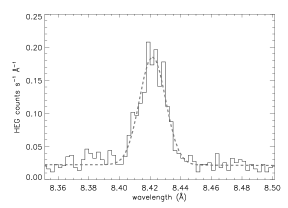
Figure 7: The Mg Lyman-$\alpha$ line in the combined Chandra HEG spectrum from all four observations (solid histogram, both panels). A model with only thermal broadening ($v_{\rm th}=104$ km s^-1; dashed line, upper panel) is much narrower than the observed profile. A Gaussian line model wth thermal and turbulent broadening due to bulk motion ($\xi=328$ km s^-1; dashed line, lower panel) provides a better fit to the data.

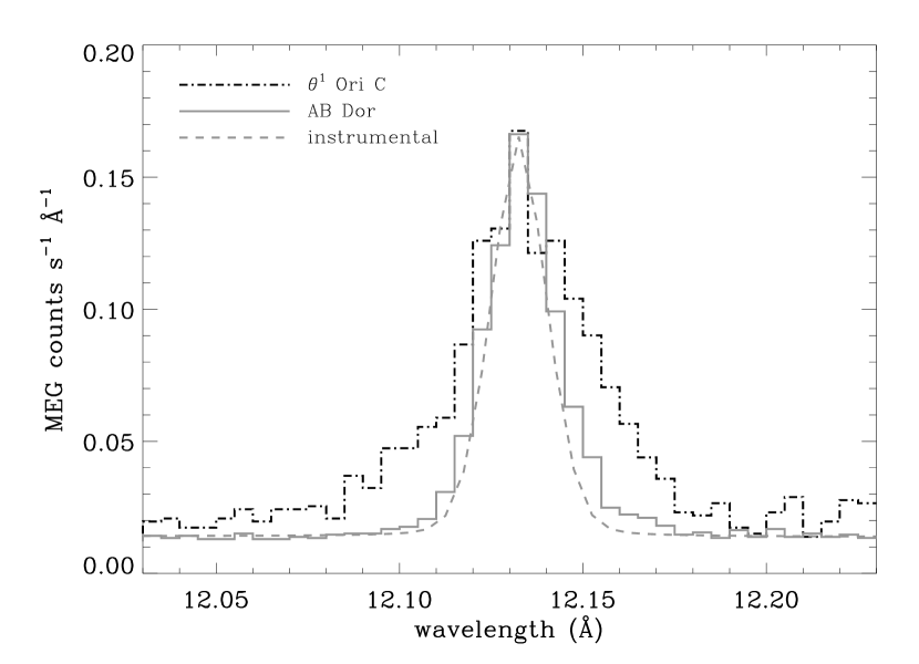
Figure 8: The Ne Lyman-$\alpha$ line in the combined Chandra MEG spectrum from all four observations of $\theta^{1}$ Ori C (solid histogram) compared to the same line seen in the MEG spectrum of the active young K-type dwarf, AB Doradus (dash-dot histogram). An delta function convolved with the MEG instrumental response (dashed line) is also shown for comparison. The $\theta^{1}$ Ori C line is clearly broader than both the narrow line or the AB Dor line.

With the detailed analysis we carried out and described in §2, we find finite, but not large, line widths, as indicated in Table 2. The lines are clearly resolved, as we show in Figures 7 and 8, in which two strong lines, one in the HEG and one in the MEG, are compared to intrinsically narrow models, Doppler-broadened models, and also to data from a late-type star with narrow emission lines.

We took a significant amount of care in deriving the line widths, fitting all lines in a given complex and carefully accounting for continuum emission. We fit each of the four observations separately, but generally find consistent widths from observation to observation, as we discuss below. In Figure 9, the Doppler width $v_{\rm D}$ of each line (open circles) is plotted versus the peak $\log T$ of that line. The rms turbulent velocities $\xi$ are plotted as filled diamonds. The Doppler widths are slightly higher than the rms velocities because the Doppler width includes the effects of thermal broadening. The velocities do not appear to depend on temperature, however there are two anomalous line profiles. The O VIII Lyman-$\alpha$ at 18.97 Å ($\xi\approx 850$ km s^-1) and Fe XVII at 15.01 Å ($\xi\approx 700$ km s^-1) are substantially broader than any of the other lines. Excluding these two lines, we find a mean $v_{\rm D}=351\pm 72$ km s^-1 and a mean $\xi=345\pm 88$ km s^-1. Because O VIII and Fe XVII tend to form at lower temperatures ($T\approx 5\times 10^{6}$) the two broader lines could represent cooler plasma formed by the standard wind instability process. Approximately 80% of the total emission measure is in the hotter 30 MK plasma. For lines formed in this hotter plasma, the Doppler broadening is substantially lower than the wind velocity. The modeled line widths from the MHD simulations, however, are quantitatively consistent with the results derived from the data.

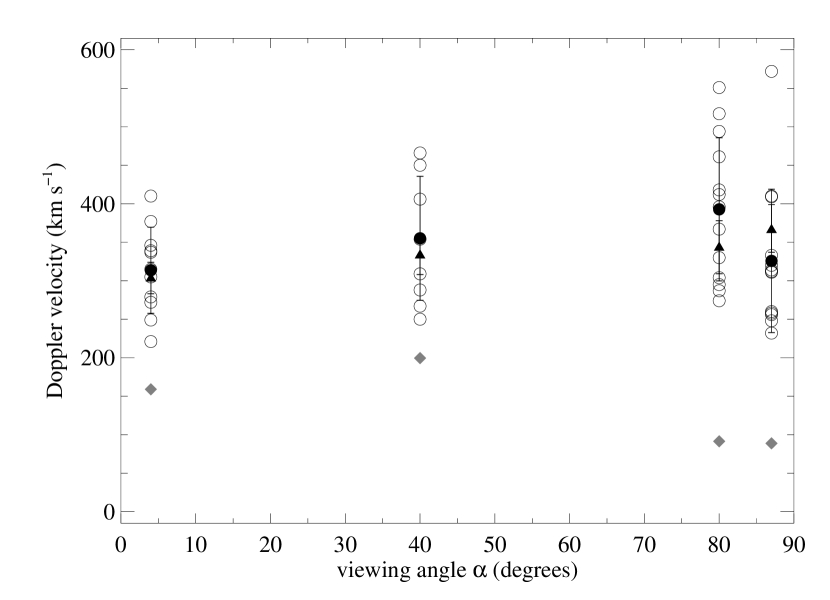
Figure 10: Line widths for the strongest lines in the Chandra spectra (open circles) at each of our four observations. The filled circles are the mean measured line widths and the error bars are the standard deviations of the mean values. The gray diamonds are the theoretical predictions based on the MHD simulations. The velocity widths plotted here are the Doppler width components, $v_{D}$, as described in §2. Note that the observed lines are somewhat broader than predicted by the MHD simulations, but substantially less broad than expected from line-driven shocks in the wind.

The line widths we derive from the data are relatively, but not totally, narrow, and they are also approximately constant as a function of rotational phase and magnetic field viewing angle. We show these results in Figure 10. This is somewhat surprising in the context of the MCWS model as elucidated by Babel & Montmerle (1997b) and Donati et al. (2002), where the pole-on viewing angle is expected to show more Doppler broadening, as the shock-heated plasma should be moving toward the magnetic equatorial plane along the observer’s line of sight. However, as we showed in §4, the full numerical simulations predict non-thermal line widths of 100–250 km s^-1. In Fig. 10 we show the Doppler velocity from a simulation when the magnetosphere was stable (cf. Fig. 5) as gray filled diamonds.

Finally, the dynamics of the shock-heated plasma in the MCWS model might be expected to lead to observed line centroid shifts with phase, or viewing angle. This would be caused by occultation of the far side of the magnetosphere by the star or by absorption in the cooling disk (see Donati et al. (2002)).

As predicted by the MHD simulations, the data show line centroids very close to zero velocity at all viewing angles. Note, though, the global fits discussed in §5.3 show evidence for a small viewing-angle dependence.

5.2 Helium-like Forbidden-to-Intercombination Line Ratios

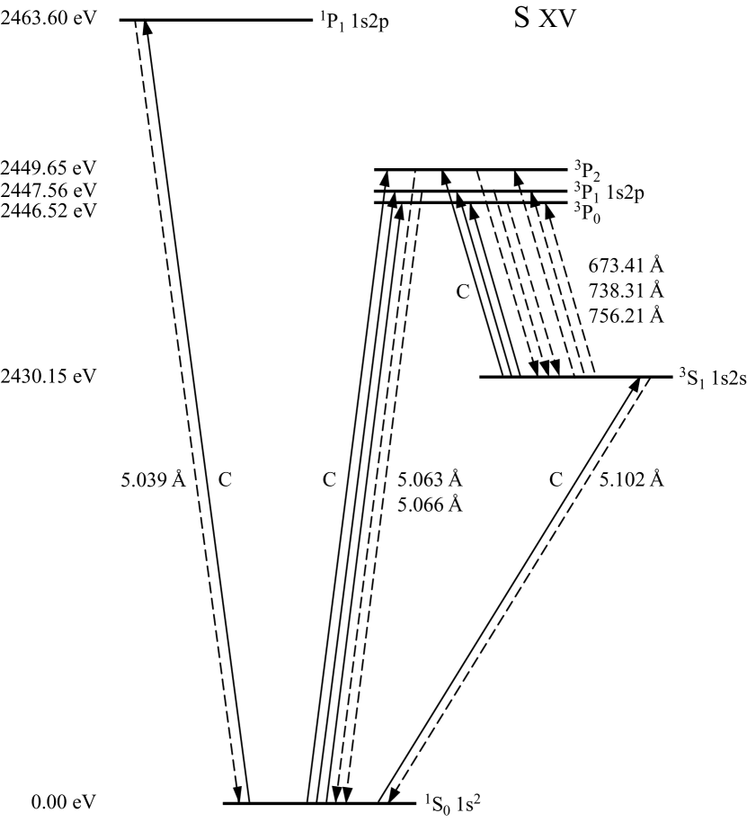
Figure 11: Energy-level diagram for S XV, based on the O VII diagram of Gabriel & Jordan (1969). Collisional excitations (C) are shown as upward pointing solid lines; radiative decays are shown as downward pointing dashed lines; photoexcitations are shown as upward pointing dashed lines. APED level energies and observed transition wavelengths are also shown. Electrons are excited out of the metastable ${}^{3}{\rm S_{1}}$ state by collisions at high density and by radiation close to a hot photosphere.

The ratio of forbidden-to-intercombination ($f/i$) line strength in helium-like ions can be used to measure the electron density of the X-ray emitting plasma and/or its distance from a source of FUV radiation, like the photosphere of a hot star (Blumenthal, Drake, & Tucker, 1972). Figure 11 is an energy-level diagram for S XV similar to the one for O VII first published by Gabriel & Jordan (1969). It shows the energy levels (eV) and transition wavelengths (Å) from APED of the resonance (${}^{1}{\rm P}_{1}\rightarrow~{}^{1}{\rm S}_{0}$), intercombination (${}^{3}{\rm P}_{2,1}\rightarrow~{}^{1}{\rm S}_{0}$), and forbidden (${}^{3}{\rm S}_{1}\rightarrow~{}^{1}{\rm S}_{0}$) lines. Aside from the usual ground-state collisional excitations (solid lines) and radiative decays (dashed lines), the metastable ${}^{3}{\rm S_{1}}$ state can be depopulated by collisional and/or photoexcitation to the ${}^{3}{\rm P}$ states. In late-type stars, the $f/i$ ratios of low-Z ions like N VI and O VII are sensitive to changes in electron density near or above certain critical densities (typically in the $10^{12}$ cm^-3 regime). Higher-Z ions have higher critical electron densities usually not seen in normal (non-degenerate) stars. Kahn et al. (2001) have used the $f/i$ ratios of N VI, O VII, and Ne IX and the radial dependence of the incident UV flux to determine that most of the emergent X-rays from the O4 supergiant $\zeta$ Pup were formed in the far wind, consistent with radiately driven wind shocks.

In our observations of $\theta^{1}$ Ori C, the He-like lines of Fe XXV, Ca XIX, Ar XVII, S XV, Si XIII, and Mg XI, were detected at all phases. However, accurate $f/i$ ratios cannot be determined for all ions. The resonance and intercombination lines of Fe XXV at 1.850 Å and Ca XIX at 3.177 Å are blended in the HEG, and weak or non-existent in the MEG. Similarly, Ne IX at 13.447 Å and O VII at 21.602 Å are weak or non-existent in the HEG.

Derived forbidden-to-intercombination ($f/i$) and forbidden-plus-intercombination-to-resonance $(f+i)/r$ ratios are listed in Table 4. The Mg XI, Ne IX, and O VII forbidden lines are completely suppressed via FUV photoexcitation of the ${}^{3}{\rm S}_{1}$ upper level, while the forbidden lines of Si XIII, S XV, and Ar XVII are partially suppressed. Fig. 12 shows the He-like line complexes of Ar XVII, S XV, Si XIII, Mg XI with their best fit models. The forbidden lines of O VII and Ne IX (not shown in Fig. 12) are completely suppressed.

The Ar XVII forbidden line at 3.994 Å is blended with S XVI Lyman-$\beta$ at 3.990 and 3.992 Å and S XV at 3.998 Å. Based on the ISIS abundances and emission-measures (see §5.3 below), APED predicts that only 26% of the HEG line flux comes from the Ar XVII $f$ line. In the above case, the $f/i$ ratio is highly uncertain and strongly model dependent, making the use of this line ratio problematic. The Si XIII $f$ line at 6.740 Å is blended with the Mg XII Ly$\gamma$ doublet at 6.738 Å. Similarly, we estimate that the Mg XII doublet’s flux is approximately $11.8\times 10^{-6}$ ph cm^-2 s^-1, approximately 38% of the flux at 6.740 Å. Assigning the remaining flux to the Si XIII $f$ line results in $f/i$ = 0.98, where we have assigned a large 30% uncertainty in Table 4 because of the blending problem.

This leaves us with $f/i$ measurements for Mg XI, S XV, as well as Si XIII. We take the Mg forbidden line to be undetected (the fit result in Table 4 shows that it is just barely detected at the $1\sigma$ level). The sulfur $f/i$ value is quite well constrained, though, and lies somewhere between the two limits (generally referred to as “high density” and “low density,” reflecting the traditional use of this ratio as a density diagnostic in purely collisional plasmas).

Of course, the photospheric emergent fluxes must be known at the relevant UV wavelengths for the $f/i$ ratio to determine the location of the X-ray emitting plasma. The Mg XI, Si XIII and S XV photoexcitation wavelengths are listed in Table 4. The 1034 Å flux has been measured using archival Copernicus spectra. For the fluxes short of the Lyman limit at 912 Å where we have no data and for which non-LTE model atmospheres and synthetic spectra have not been published, we scaled the flux from a 45000 K blackbody (the hot model in Table 3). We computed the $f/i$ ratios using the PrismSPECT non-LTE excitation kinematics code (MacFarlane, Golovkin, Woodruff, & Wang, 2003). For each line complex, we set up a model atom with several dozen levels for each ion using oscillator strengths and transition rates custom-computed using Hartree-Fock and distorted wave methodologies. The resulting values were checked against data from the literature. We include collisional and radiative coupling among most levels in the model atom, and specifically include photoexcitation between the ${}^{3}{\rm S_{1}}$ and ${}^{3}{\rm P}$ levels driven by photospheric radiation.

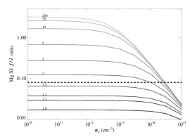
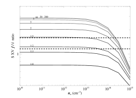
Figure 13: He-like $f/i$ ratio versus $n_{\rm e}$ at various radii from 1–200 $R_{\star}$, assuming a 45000 K photosphere, for Mg XI (upper panel) and S XV (lower panel). The measured $f/i$ upper and lower bounds from Table 4 are shown as dashed lines. The Mg XI, Si XIII, and S XV suggest a formation radius, $1.2R_{\star}\leq R\leq 1.5R_{\star}$.

The results of this modeling for Mg XI and S XV are shown in Figure 13, where the solid lines represent $f/i$ as a function of electron density for a range of radii from 1–200 $R_{\star}$. The dashed line in Fig. 14a is the Mg XI upper limit, indicating an upper limit to the formation radius $R\leq 1.7R_{\star}$. The dashed lines in Fig. 14b are the S XV $1\sigma$ upper and lower bounds, indicating a formation radius in the range $1.2R_{\star}\leq R\leq 1.5R_{\star}$. The resulting bounds from Si XIII are consistent with S XV. Of course, it is a simplification to assume that all of the plasma (even for a given element or ion stage) is at a single radius. The formation radii we have derived should thus be thought of as an emission-measure weighted mean. In any case, it is clear that the hot plasma in the circumstellar environment of $\theta^{1}$ Ori C is quite close to the photosphere. We note that there is no variation in the average formation radius among the four separate phase observations. We note that these results are comparable to those found by Schulz et al. (2003) based on the ealier two data sets.

5.3 Emission-Measure and Abundance Variability

There are several additional diagnostics that involve analysis not of the properties of single lines, but of the X-ray spectrum as a whole. The global thermal model fitting with ISIS described in §2 yields abundance and emission-measure information, while the line flux values taken as an ensemble can be analyzed for phase, or viewing angle, dependence. Detailed descriptions of these analyses have already been presented §2, so here we simply present the results.

The elemental abundances derived from the two different fitting methods are reported in Table 5. Most elemental abundances do not deviate significantly from solar, although Fe is well below solar and several intermediate atomic number elements are slightly above solar.

The HEG/MEG spectra for each observation were fit with a variable-abundance, 2-temperature ISIS plasma model with radial velocity and turbulent (a.k.a., rms) velocity as free parameters (See Table 6), with a single column density parameter, $N_{\rm H}$. We tried fitting the individual and combined spectra with 2-, 5-, and 21-temperature APEC models with solar and non-solar abundances. No solar-abundance model can adequately fit the continuum and emission lines. The 5- and 21-temperature component models do not provide appreciably better fits than the 2-temperature non-solar abundance model. Although plasma at a number of temperatures may be present, it is not possible to accurately fit so many free parameters with moderate S/N HETG data.

Schulz et al. (2003) used a six-temperature, variable abundance APEC plasma model to fit the combined HEG/MEG spectra from OBSID 3 and 4. They find $N_{\rm H}\approx 5\times 10^{21}$ cm^-2, sub-solar Fe, Ni, O and Ne and approximately solar abundances of other elements, again, consistent with our results in Table 6. Their Figure 7, however, suggests a phase dependence in the six-temperature emission-measure distribution, which we cannot confirm. We point out, however, that the $1\sigma$ error envelope in their emission-measure distributions overlap significantly. The emission measures in Table 6 for phases 0.38 and 0.84 appear to fit within both EM envelopes in Fig. 7 of Schulz et al. (2003).

The visible emission measure decreases by 36% from X-ray maximum to minimum, suggesting a substantial fraction of the X-ray emitting region is occulted by the star at high viewing angles. Comparison between the observed data and the MHD simulations show the agreement is quite good, both in terms of the overall volume emission measure and in its temperature distribution.

As has previously been shown (Gagné et al., 1997; Babel & Montmerle, 1997b; Donati et al., 2002), the phase dependence of the X-ray spectrum provides information about the extent and location of the X-ray emission and absorption in the wind and disk. There are no large, systematic spectral variations at the four phases observed with Chandra. E.g., the soft X-ray portion of the MEG is not more absorbed than the hard X-ray portion, suggesting that the variability is not primarily caused by absorption in the disk or by a polar wind. Rather it appears that most of the variability is caused by occultation of the X-ray emitter by the stellar photosphere as the magnetically confined region rotates every 15.4 days.

That said, there does a appear to be a small increase in column density when the disk is viewed nearly edge-on. Figure 14 shows the ISIS parameters, $N_{\rm H}$ (upper curve, right axis) and radial velocity (lower curve, left axis), as a function of viewing angle. The excess column density, $N_{\rm H}\approx 5\times 10^{20}$ cm^-2, would arise as a result of increased outflow in the magnetic equatorial plane. Because increased column density and increased temperature harden the predicted X-ray spectrum in somewhat similar ways, we consider the column density variablity as a tentative result. We point at that X-ray absorption towards $\theta^{1}$ Ori C occurs in the ISM, in the neutral lid of the Orion Nebula, in the ionized cavity, and in the stellar wind. The Wisconsin absorption model for cold interstellar gas yields a single column density parameter that does not take into account the ionization fraction, temperature and abundance of these absorption components.

The measured radial velocities at viewing angles $4\arcdeg$ (pole-on), $39\arcdeg$, $80\arcdeg$, and $87\arcdeg$ (edge-on) were $-75\pm 10$, $-66^{+12}_{-9}$, $19^{+19}_{-18}$, and $93^{+16}_{-13}$ km s^-1, respectively. Systematic line shifts were not detected in individual line complexes (see §5.1) because the uncertainty in the centroid velocity of a single line is higher than its uncertainty based on a large number of lines. For instance, the $1\sigma$ uncertainty at each OBSID in the line centroid of Fe XVII $\lambda 15.014$ is approximately 50 km s^-1.

The simulations predict no significant blueshifts or redshifts at any viewing angle. As a result, the $-75$ km s^-1 blueshift at low viewing angle and the $+93$ km s^-1 redshift at high viewing angle seen in Fig. 11, if real, may lead to further improvements of the model. The 2D MHD simulations show that the hot plasma is constantly moving, sometimes falling back to the photosphere in one hemisphere or the other, other times expanding outward in the magnetic equatorial plane following reconnection events. Because the four Chandra observations were obtained months or years apart, the radial velocity variations may reflect the stochastic nature of the X-ray production mechanism or persistent flows of shock-heated plasma.

Though small, the X-ray line shifts nicely match the C IV, N V and H$\alpha$ emission components discussed by Smith & Fullerton (2005). In this picture, material falling back onto the photosphere along closed magnetic field lines produces redshifted emission when viewed edge-on. The blueshifted X-ray and H$\alpha$ emission seen at low viewing angles (pole-on, $\phi=0$) would be produced by (1) the same infalling plasma viewed from an orthogonal viewing angle and/or (2) by material in the outflowing wind. Smith & Fullerton (2005) argue that a polar outflow probably cannot produce the observed levels of H$\alpha$ and He II $\lambda 4686$ emission, thereby preferring the infall scenario.

If pole-on blueshifts in the X-ray lines are persistent, this suggests asymmetric infall towards the north (near) magnetic pole. Such blueshifts could be caused by an off-centered oblique dipole. The blueshifts might also be caused by absorption of the red emission in the far hemisphere by the cooler post-shock gas. However, this would produce weaker X-rays at pole-on phases. Since stronger X-ray emission is observed at pole-on phases, asymmetric infall provides a better explanation for the blueshifted H$\alpha$ and X-ray line emission. Repeated observations at pole-on and edge-on phases are needed to confirm this result.

6 Discussion

The high-resolution X-ray spectroscopy covering the full range of magnetospheric viewing angles adds a significant amount of new information to our understanding of the high energy processes in the circumstellar environment of $\theta^{1}$ Ori C, especially when interpreted in conjunction with data from other wavelength regions and our new MHD numerical simulations. As the simplified MCWS modeling (Babel & Montmerle, 1997b; Donati et al., 2002) indicated and our detailed MHD simulations confirmed, the magnetically channeled wind model can produce the right amount of X-rays and roughly the observed temperature distribution in the X-ray emitting plasma. The two new Chandra observations we report on in this paper reinforce the global spectral information already gleaned from the two GTO observations. In addition, the better phase coverage now shows that the modulation of the X-rays is quite gray, indicating that occultation by the star at phases when our view of the system is in the magnetic equatorial plane, is the primary cause of the overall X-ray variability. Incidentally, the fact that the reduction in the flux is maximal at $\phi=0.5$ confirms the reassessment of field geometry by Donati et al. (2002).

The fractional decrease in the observed flux of roughly 35%, interpreted in the context of occultation, indicates that the X-ray emitting plasma is quite close to the photosphere: $1.2R_{\star}\leq R\leq 1.4R_{\star}$. This result is completely consistent with the observed Mg XI, Si XIII and S XV $f/i$ values, which together indicate $1.2R_{\star}\leq R\leq 1.5R_{\star}$, i.e., between 0.2 and 0.5 stellar radii above the photosphere. The MHD simulations we have performed also show the bulk of the very hot emission measure to be, on average, within $2R_{\star}$.

We see evidence for slightly enhanced attenuation at large viewing angles (nearly edge-on) as a result of wind material channeled into the magnetic equatorial plane. We should point out that the infall (in the closed-field region) and outflow (in the open-field region) means that a dense, X-ray absorbing, cooling disk does not form in the equatorial plane.

The X-ray emission lines seen in the Chandra spectra are well resolved, but relatively narrow, and show small ($<100$ km s^-1) centroid shifts. Although the 2D MHD simulations indicate little or no line shifts on average, the small observed shifts (also seen in H$\alpha$) may reflect the stochastic nature of the infall onto the star. If the blueshifts at pole-on phases are persistent, they may indicate an asymmetry in the magnetic/wind geometry.

The line widths in the simulations are even narrower than those seen in the data. But this is, perhaps, not too surprising, as the simulations do not include the deshadowing instability that can lead to shock heating in the bulk wind. Some radiatively-driven X-ray production in the cooler ($T\approx 6\times 10^{6}$ K) wind shocks was suggested by Schulz et al. (2003) and may explain the larger widths of the Fe XVII and O VIII lines. Furthermore, fully three dimensional simulations may reveal additional turbulence or other bulk motions.

7 Conclusions

The magnetically channeled wind shock model for magnetized hot stars with strong line-driven winds provides excellent agreement with the diagnostics from our phase-resolved Chandra spectroscopy of $\theta^{1}$ Ori C. The modest line widths are consistent with the predictions of our MHD simulations. The X-ray light curve and He-like $f/i$ values indicate that the bulk of the X-ray emitting plasma is located at approximately $1.5R_{\star}$, very close to the photosphere, which is also consistent with the MHD simulations of the MCWS mechanism. The simulations also correctly predict the temperature and total luminosity of the X-ray emitting plasma. We emphasize that the only inputs to the MHD simulations were the magnetic field strength, effective temperature, radius, and mass-loss rate of $\theta^{1}$ Ori C, all of which are fairly well constrained by observation.

Although the original explorations of the MCWS mechanism indicated that there might be significant viewing angle dependencies in some of these diagnostics, the numerical simulations by and large do not predict them, and they are generally not seen in the data. Spatial stratification of the very hottest plasma might explain the slight wavelength dependence of the viewing angle variability of the X-ray flux.

The new MHD simulations we present for $\theta^{1}$ Ori C are similar to the original calculations by ud-Doula & Owocki (2002), but the more accurate treatment of the energy equation makes for some modest changes, and allows for a direct prediction of its X-ray emission properties. Future, fully 3D simulations might show even better agreement with the data if different longitudinal sectors of the magnetosphere exhibit independent dynamics. But the addition of rotation into the dynamical equations of motion probably is not important for this star and seems to be unnecessary for reproducing the observations.

The red and blue wings of the C IV and N V UV resonance-lines, the optical H I Balmer and He II lines, and small centroid velocity shifts in the X-ray lines may point to more complicated, episodic infall and/or mass-loss.

As was pointed out by Schulz et al. (2003), $\theta^{1}$ Ori C is one of many early-type stars in OB associations with hard X-ray spectra. The MCWS model may be fruitfully applied to $\tau$ Sco, and other young, early-type stars that show relatively narrow X-ray emission lines, hard X-ray spectra, and time variability.

Figure 1: Schematic of $\theta^{1}$ Ori C and its circumstellar environment. The curved lines represent a set of magnetic field lines stretched out by the wind. The vector indicates the magnetic axis and the dashed line represents the magnetic equatorial plane. The viewing angles in degrees with respect to the magnetic axis of the four Chandra observations, $\alpha$, are indicated by the four labels, 4, 40, 80, and 87. The arrows point to the observer. In this figure, taken from the perspective of the star’s magnetic axis, the observer appears to move from $\alpha\approx 3\arcdeg$ (at rotational phase 0.0) to $\alpha\approx 87\arcdeg$ (at rotational phase 0.5), back to $\alpha\approx 3\arcdeg$ (at rotational phase 1.0) as a result of the magnetic obliquity, $\beta=42\arcdeg$. The rotation axis, which we assume is inclined by approximately $45\arcdeg$ to the observer, is not shown because it too would move. The hard X-ray emitting region is shown schematically as a gray torus. At high viewing angles, the entire torus is visible (X-ray maximum). At low viewing angles, some of the torus is occulted (X-ray minimum).

Figure 2: All four co-added, first order MEG spectra, ordered according to viewing angle (pole-on to equator-on). The bottom panel shows an averaged MEG spectrum composed of the four individual spectra. The low count rate at long wavelengths is due to ISM attenuation.

Figure 3: All four co-added, first order HEG spectra, ordered according to viewing angle (pole-on to equator-on). The bottom panel shows an averaged HEG spectrum composed of the four individual spectra. The HEG has higher spectral resolution than the MEG, but lower throughput longward of approximately 3.5 Å.

Figure 4: Phase-folded light curves of $\theta^{1}$ Ori C. Upper panel: open circles indicate the excess C IV equivalent width (left axis) taken from Walborn & Nichols (1994) and phased to the ephemeris of Stahl et al. (1996): period $P=15.422$ days and epoch ${\rm MJD}_{0}$ = 48832.50. Maximum C IV absorption occurs near phase 0.5 ($\alpha=3\arcdeg$) as a result of outflowing plasma in the magnetic equatoral plane. Note: Walborn & Nichols (1994) calculate $W_{\lambda}$ by subtracting the IUE spectrum at a given phase from the IUE spectrum with the shallowest line profile, then calculating the equivalent width of the line in the difference spectrum. Filled circles show the longitudinal magnetic field strength, $B_{\ell}$, (right axis) as measured by Donati et al. (2002) using the same ephemeris. Note that Walborn & Nichols (1994) and Donati et al. (2002) used different period estimates. $B_{\ell}$ is maximum near phase 0.0 when the magnetic pole is in the line of sight. Lower panel: H$\alpha$ equivalent width (solid curve) from Stahl et al. (1996). The data points with error bars represent the ACIS-I count rate from the 850-ks Chandra Orion Ultra-Deep Project. X-ray and H$\alpha$ maxima occur at low viewing angles when the entire X-ray torus is visible; the minima occur when part of the X-ray torus is occulted by the star.

Figure 5: Grayscale (print edition) and color (electronic edition) snapshots from the 500-ks, slow-wind, 2D MHD simulation of $\theta^{1}$ Ori C, superposed with corresponding magnetic field lines. Upper panel: logarithm of the emission measure per unit volume, $\log n_{\rm e}n_{\rm H}$. Lower panel: logarithm of temperature, $\log T$. In this snapshot, obtained at simulation time $t=375$ ks, material trapped in closed loops is falling back toward the stellar surface along field lines, forming a complex “snake-like” pattern. The regions of highest emission measure in the 1–100 MK temperature range occur above and below the magnetic equator, close to $R\approx 2R_{\star}$.

Figure 6: Volume emission-measure distribution per $\log T=0.1$ bin, from the snapshot in Fig. 5. The MHD simulation is used to compute the emission-measure per unit volume per logarithmic temperature bin, then integrated over 3D space assuming azimuthal symmetry about the magnetic dipole axis. The total simulated volume emission measure in the interval $6.0\leq\log T<8.0$ exceeds the total emission measure seen with the HETG by a factor of two. The low-velocity wind ($v_{\infty}\approx 1470$ km s^-1) simulation in Fig. 5 also produces a slightly cooler distribution of shocks than observed. Full 3D MHD simulations may be needed to resolve these discrepancies.

Figure 9: Line widths for the strongest lines in the Chandra spectra plotted against the temperature of peak line emissivity, taken from APED. The open circles represent the Doppler width as measured by SHERPA. The filled diamonds represent the rms velocity as measured by ISIS. The mean rms velocity and standard deviations of these lines are indicated by the horizontal lines. Note that two of the lines formed in the coolest plasma are significantly broader than the mean, but that most of the lines have non-thermal line widths of a 250–450 km s^-1.

Figure 14: The HEG/MEG spectra show slight changes in radial velocity (left axis, filled circles) and column density (right axis, open circles) from observation to observation. At low viewing angles (pole-on), the X-ray lines are slightly blueshifted; at high viewing angles (disk-on), the lines are redshifted with a hint of excess absorption from ionized gas in the disk. The increased absorption may indicate outflowing wind material in the magnetic equatorial plane. The redshifts and blueshifts may indicate obliquely infalling material seen from various viewing angles.

Table 1: Chandra Observations of $\theta^{1}$ Ori C

Sequence	Observation	Detector/	Start Date	End Date	Exposure	Average	Viewing
Number	ID	Grating	Start Time (UT)	End Time (UT)	Time (ks)	Phase	Angle
200001	3	ACIS-S HETG	31 Oct 1999 05:47:21	31 Oct 1999 20:26:13	052.0	0.84	$40^{\circ}$
200002	4	ACIS-S HETG	24 Nov 1999 05:37:54	24 Nov 1999 15:08:39	033.8	0.38	$80^{\circ}$
200175	2567	ACIS-S HETG	28 Dec 2001 12:25:56	29 Dec 2001 02:00:53	046.4	0.01	$\phantom{0}4^{\circ}$
200176	2568	ACIS-S HETG	19 Feb 2002 20:29:42	20 Feb 2002 10:01:59	046.3	0.47	$87^{\circ}$
200214	4395	ACIS-I NONE	08 Jan 2003 20:58:19	10 Jan 2003 01:28:41	100.0	0.44	$85^{\circ}$
200214	3744	ACIS-I NONE	10 Jan 2003 16:17:39	12 Jan 2003 14:51:52	164.2	0.58	$84^{\circ}$
200214	4373	ACIS-I NONE	13 Jan 2003 07:34:44	15 Jan 2003 08:12:49	171.5	0.75	$58^{\circ}$
200214	4374	ACIS-I NONE	16 Jan 2003 00:00:38	17 Jan 2003 23:56:05	169.0	0.92	$19^{\circ}$
200214	4396	ACIS-I NONE	18 Jan 2003 14:34:49	20 Jan 2003 13:15:31	164.6	0.09	$23^{\circ}$
200193	3498	ACIS-I NONE	21 Jan 2003 06:10:28	22 Jan 2003 02:09:20	069.0	0.23	$54^{\circ}$

Table 2: HEG and MEG Line List for $\theta^{1}$ Ori C: Combined Observations

Ion	Transition	$\lambda_{0}$	$\lambda$	$\sigma_{\lambda}$	$10^{6}f_{\ell}$	$10^{6}\sigma_{f}$	$v_{D}$	$\sigma_{v}$	$\xi$	$\sigma_{\xi}$
		(Å)	(Å)	(Å)	(ph cm-2s-1)		(km s-1)		(km s-1)
Fe XXV	$1s2p~{}^{1}P_{1}\rightarrow 1s^{2}~{}^{1}S_{0}$	1.8504	1.8498	0.0009	26.23	4.86	409	$\cdots$	300	$\cdots$
Fe XXV	$1s2p~{}^{3}P_{2}\rightarrow 1s^{2}~{}^{1}S_{0}$	1.8554	1.8548	$\cdots$	10.00	2.62	409	$\cdots$	300	$\cdots$
Fe XXV	$1s2p~{}^{3}P_{1}\rightarrow 1s^{2}~{}^{1}S_{0}$	1.8595	1.8589	$\cdots$	9.57	$\cdots$	409	$\cdots$	300	$\cdots$
Fe XXV	$1s2s~{}^{3}S_{1}\rightarrow 1s^{2}~{}^{1}S_{0}$	1.8682	1.8676	$\cdots$	28.47	4.56	409	$\cdots$	300	$\cdots$
Ca XIX	$1s2p~{}^{1}P_{1}\rightarrow 1s^{2}~{}^{1}S_{0}$	3.1772	3.1746	0.0013	8.70	1.62	426	263	300	$\cdots$
Ca XIX	$1s2p~{}^{3}P_{2}\rightarrow 1s^{2}~{}^{1}S_{0}$	3.1891	3.1865	$\cdots$	4.32	0.88	426	$\cdots$	300	$\cdots$
Ca XIX	$1s2p~{}^{3}P_{1}\rightarrow 1s^{2}~{}^{1}S_{0}$	3.1927	3.1901	$\cdots$	3.66	$\cdots$	426	$\cdots$	300	$\cdots$
Ca XIX	$1s2s~{}^{3}S_{1}\rightarrow 1s^{2}~{}^{1}S_{0}$	3.2110	3.2083	$\cdots$	6.93	1.52	426	$\cdots$	300	$\cdots$
Ar XVIII	$2p~{}^{2}P_{3/2}\rightarrow 1s~{}^{2}S_{1/2}$	3.7311	3.7308	0.0016	6.48	1.16	400	$\cdots$	400	$\cdots$
Ar XVIII	$2p~{}^{2}P_{1/2}\rightarrow 1s~{}^{2}S_{1/2}$	3.7365	3.7362	$\cdots$	3.10	$\cdots$	400	$\cdots$	400	$\cdots$
Ar XVII	$1s2p~{}^{1}P_{1}\rightarrow 1s^{2}~{}^{1}S_{0}$	3.9491	3.9489	0.0009	13.02	1.91	413	132	300	$\cdots$
Ar XVII	$1s2p~{}^{3}P_{2}\rightarrow 1s^{2}~{}^{1}S_{0}$	3.9659	3.9657	$\cdots$	3.38	0.75	413	$\cdots$	300	$\cdots$
Ar XVII	$1s2p~{}^{3}P_{1}\rightarrow 1s^{2}~{}^{1}S_{0}$	3.9694	3.9692	$\cdots$	3.46	$\cdots$	413	$\cdots$	300	$\cdots$
S XVI	$3p~{}^{2}P_{3/2}\rightarrow 1s~{}^{2}S_{1/2}$	3.9908	3.9906	$\cdots$	2.44	$\cdots$	413	$\cdots$	300	$\cdots$
S XVI	$3p~{}^{2}P_{1/2}\rightarrow 1s~{}^{2}S_{1/2}$	3.9920	3.9918	$\cdots$	1.22	$\cdots$	413	$\cdots$	300	$\cdots$
Ar XVII	$1s2s~{}^{3}S_{1}\rightarrow 1s^{2}~{}^{1}S_{0}$	3.9942	3.9940	$\cdots$	12.37	1.95	413	$\cdots$	300	$\cdots$
S XVI	$2p~{}^{2}P_{3/2}\rightarrow 1s~{}^{2}S_{1/2}$	4.7274	4.7270	0.0006	41.28	2.21	539	77	478	82
S XVI	$2p~{}^{2}P_{1/2}\rightarrow 1s~{}^{2}S_{1/2}$	4.7328	4.7324	$\cdots$	19.73	$\cdots$	539	$\cdots$	478	$\cdots$
S XV	$1s2p~{}^{1}P_{1}\rightarrow 1s^{2}~{}^{1}S_{0}$	5.0387	5.0382	0.0005	50.53	3.15	331	55		$\cdots$
S XV	$1s2p~{}^{3}P_{2}\rightarrow 1s^{2}~{}^{1}S_{0}$	5.0631	5.0626	$\cdots$	6.54	0.98	331	$\cdots$	$\cdots$	$\cdots$
S XV	$1s2p~{}^{3}P_{1}\rightarrow 1s^{2}~{}^{1}S_{0}$	5.0665	5.0660	$\cdots$	9.39	$\cdots$	331	$\cdots$	$\cdots$	$\cdots$
S XV	$1s2s~{}^{3}S_{1}\rightarrow 1s^{2}~{}^{1}S_{0}$	5.1015	5.1010	$\cdots$	21.92	2.51	331	$\cdots$	$\cdots$	$\cdots$
Si XIV	$2p~{}^{2}P_{3/2}\rightarrow 1s~{}^{2}S_{1/2}$	6.1804	6.1803	0.0002	75.47	1.60	355	23	305	28
Si XIV	$2p~{}^{2}P_{1/2}\rightarrow 1s~{}^{2}S_{1/2}$	6.1858	6.1857	$\cdots$	36.15	$\cdots$	355	$\cdots$	305	$\cdots$
Si XIII	$1s2p~{}^{1}P_{1}\rightarrow 1s^{2}~{}^{1}S_{0}$	6.6479	6.6480	0.0003	61.40	1.88	370	21		$\cdots$
Si XIII	$1s2p~{}^{3}P_{2}\rightarrow 1s^{2}~{}^{1}S_{0}$	6.6850	6.6851	$\cdots$	14.04	1.03	370	$\cdots$	$\cdots$	$\cdots$
Si XIII	$1s2p~{}^{3}P_{1}\rightarrow 1s^{2}~{}^{1}S_{0}$	6.6882	6.6883	$\cdots$	5.40	$\cdots$	370	$\cdots$	$\cdots$	$\cdots$
Mg XII	$4p~{}^{2}P_{3/2}\rightarrow 1s~{}^{2}S_{1/2}$	6.7378	6.7379	$\cdots$	7.86	$\cdots$	370	$\cdots$	$\cdots$	$\cdots$
Mg XII	$4p~{}^{2}P_{1/2}\rightarrow 1s~{}^{2}S_{1/2}$	6.7382	6.7383	$\cdots$	3.93	$\cdots$	370	$\cdots$	$\cdots$	$\cdots$
Si XIII	$1s2s~{}^{3}S_{1}\rightarrow 1s^{2}~{}^{1}S_{0}$	6.7403	6.7404	$\cdots$	18.98	1.45	370	$\cdots$	$\cdots$	$\cdots$
Mg XII	$3p~{}^{2}P_{3/2}\rightarrow 1s~{}^{2}S_{1/2}$	7.1058	7.1039	0.0009	10.97	0.77	360	54	311	54
Mg XII	$3p~{}^{2}P_{1/2}\rightarrow 1s~{}^{2}S_{1/2}$	7.1069	7.1050	$\cdots$	5.25	$\cdots$	360	$\cdots$	311	$\cdots$
Fe XXIV	$1s^{2}5p~{}^{2}P_{3/2}\rightarrow 1s^{2}2s~{}^{2}S_{1/2}$	7.1690	7.1687	0.0010	8.49	0.74	360	$\cdots$	311	$\cdots$
Fe XXIV	$1s^{2}5p~{}^{2}P_{1/2}\rightarrow 1s^{2}2s~{}^{2}S_{1/2}$	7.1690	7.1687	$\cdots$	4.15	$\cdots$	360	$\cdots$	311	$\cdots$
Fe XXIV	$1s^{2}4p~{}^{2}P_{3/2}\rightarrow 1s^{2}2s~{}^{2}S_{1/2}$	7.9857	7.9837	0.0009	13.36	0.81	363	63	336	61
Fe XXIV	$1s^{2}4p~{}^{2}P_{1/2}\rightarrow 1s^{2}2s~{}^{2}S_{1/2}$	7.9960	7.9940	$\cdots$	6.81	$\cdots$	363	$\cdots$	336	$\cdots$
Mg XII	$2p~{}^{2}P_{3/2}\rightarrow 1s~{}^{2}S_{1/2}$	8.4192	8.4183	0.0003	47.73	1.25	364	20	328	21
Mg XII	$2p~{}^{2}P_{1/2}\rightarrow 1s~{}^{2}S_{1/2}$	8.4246	8.4237	$\cdots$	22.91	$\cdots$	364	$\cdots$	328	$\cdots$
Mg XI	$1s2p~{}^{1}P_{1}\rightarrow 1s^{2}~{}^{1}S_{0}$	9.1687	9.1693	0.0007	28.89	1.68	415	49		$\cdots$
Mg XI	$1s2p~{}^{3}P_{2}\rightarrow 1s^{2}~{}^{1}S_{0}$	9.2282	9.2288	$\cdots$	2.17	0.19	415	$\cdots$	$\cdots$	$\cdots$
Mg XI	$1s2p~{}^{3}P_{1}\rightarrow 1s^{2}~{}^{1}S_{0}$	9.2312	9.2318	$\cdots$	15.20	$\cdots$	415	$\cdots$	$\cdots$	$\cdots$
Mg XI	$1s2s~{}^{3}S_{1}\rightarrow 1s^{2}~{}^{1}S_{0}$	9.3143	9.3149	$\cdots$	1.36	1.15	415	$\cdots$	$\cdots$	$\cdots$
Fe XXIV	$1s^{2}3p~{}^{2}P_{3/2}\rightarrow 1s^{2}2s~{}^{2}S_{1/2}$	10.6190	10.6205	0.0006	44.26	1.77	316	26	288	30
Fe XXIV	$1s^{2}3p~{}^{2}P_{1/2}\rightarrow 1s^{2}2s~{}^{2}S_{1/2}$	10.6630	10.6645	$\cdots$	23.28	$\cdots$	316	$\cdots$	288	$\cdots$
Fe XXIII	$1s^{2}2s3p~{}^{1}P_{1}\rightarrow 1s^{2}2s^{2}~{}^{1}S_{0}$	10.9810	10.9821	$\cdots$	25.83	1.90	300	$\cdots$	263	$\cdots$
Fe XXIII	$1s^{2}2s3p~{}^{3}P_{1}\rightarrow 1s^{2}2s^{2}~{}^{1}S_{0}$	11.0190	11.0201	$\cdots$	11.39	$\cdots$	300	$\cdots$	263	$\cdots$
Fe XXIV	$1s^{2}3d~{}^{2}D_{3/2}\rightarrow 1s^{2}2p~{}^{2}P_{1/2}$	11.0290	11.0301	0.0007	30.29	1.61	300	27	263	31
Fe XXIV	$1s^{2}3d~{}^{2}D_{5/2}\rightarrow 1s^{2}2p~{}^{2}P_{3/2}$	11.1760	11.1744	0.0006	42.87	2.13	236	33	213	38
Fe XXIV	$1s^{2}3d~{}^{2}D_{3/2}\rightarrow 1s^{2}2p~{}^{2}P_{3/2}$	11.1870	11.1854	$\cdots$	4.67	$\cdots$	236	$\cdots$	213	$\cdots$
Fe XXIII	$1s^{2}2s3d~{}^{1}D_{2}\rightarrow 1s^{2}2s2p~{}^{1}P_{1}$	11.7360	11.7413	0.0006	48.87	2.78	387	37	387	40
Fe XXII	$1s^{2}2s^{2}3d~{}^{2}D_{3/2}\rightarrow 1s^{2}2s^{2}2p~{}^{2}P_{1/2}$	11.7700	11.7753	$\cdots$	25.58	2.40	387	$\cdots$	387	$\cdots$
Ne X	$2p~{}^{2}P_{3/2}\rightarrow 1s~{}^{2}S_{1/2}$	12.1321	12.1300	0.0007	56.30	2.17	351	36	488	35
Ne X	$2p~{}^{2}P_{1/2}\rightarrow 1s~{}^{2}S_{1/2}$	12.1375	12.1354	$\cdots$	27.05	$\cdots$	351	$\cdots$	488	$\cdots$
Fe XXIII	$1s^{2}2s3s~{}^{1}S_{0}\rightarrow 1s^{2}2s2p~{}^{1}P_{1}$	12.1610	12.1589	$\cdots$	21.17	$\cdots$	351	$\cdots$	488	$\cdots$
Ne IX	$1s2p~{}^{1}P_{1}\rightarrow 1s^{2}~{}^{1}S_{0}$	13.4473	13.4386	0.0029	33.29	4.09	623	86		$\cdots$
Fe XIX	$2s^{2}2p^{3}3d~{}^{3}S_{1}\rightarrow 2s^{2}2p^{4}~{}^{3}P_{2}$	13.4620	13.4533	$\cdots$	5.93	0.61	623	$\cdots$	$\cdots$	$\cdots$
Fe XIX	$1s^{2}2s^{2}2p_{1/2}2p_{3/2}^{2}3d_{3/2}\rightarrow 2s^{2}2p^{4}~{}^{3}P_{2}$	13.4970	13.4883	$\cdots$	10.38	$\cdots$	623	$\cdots$	$\cdots$	$\cdots$
Fe XXI	$1s^{2}2s2p_{1/2}^{2}3s\rightarrow 1s^{2}2s2p^{3}~{}^{3}D_{1}$	13.5070	13.4983	$\cdots$	9.14	$\cdots$	623	$\cdots$	$\cdots$	$\cdots$
Fe XIX	$2s^{2}2p^{3}3d~{}^{3}D_{3}\rightarrow 2s^{2}2p^{4}~{}^{3}P_{2}$	13.5180	13.5093	$\cdots$	22.90	$\cdots$	623	$\cdots$	$\cdots$	$\cdots$
Ne IX	$1s2p~{}^{3}P_{2}\rightarrow 1s^{2}~{}^{1}S_{0}$	13.5503	13.5416	$\cdots$	0.99	$\cdots$	623	$\cdots$	$\cdots$	$\cdots$
Ne IX	$1s2p~{}^{3}P_{1}\rightarrow 1s^{2}~{}^{1}S_{0}$	13.5531	13.5444	$\cdots$	25.38	4.10	623	$\cdots$	$\cdots$	$\cdots$
Ne IX	$1s2s~{}^{3}S_{1}\rightarrow 1s^{2}~{}^{1}S_{0}$	13.6990	13.6903	$\cdots$	0.41	2.77	623	$\cdots$	$\cdots$	$\cdots$
Fe XX	$1s^{2}2s^{2}2p_{1/2}2p_{3/2}3p_{3/2}\rightarrow 2s2p^{4}~{}^{4}P_{3/2}$	14.9978	14.9993	$\cdots$	0.10	0.33	614	$\cdots$	700	$\cdots$
Fe XIX	$2s^{2}2p^{3}3s~{}^{1}D_{2}\rightarrow 2s^{2}2p^{4}~{}^{1}D_{2}$	15.0117	15.0132	$\cdots$	1.42	$\cdots$	614	$\cdots$	700	$\cdots$
Fe XVII	$2s^{2}2p^{5}3d~{}^{1}P_{1}\rightarrow 2s^{2}2p^{6}~{}^{1}S_{0}$	15.0140	15.0155	0.0019	82.64	5.75	614	67	700	78
Fe XX	$1s^{2}2s^{2}2p_{3/2}^{2}3p_{3/2}\rightarrow 2s2p^{4}~{}^{2}D_{5/2}$	15.0164	15.0176	$\cdots$	0.26	$\cdots$	614	$\cdots$	700	$\cdots$
Fe XVIII	$2s^{2}2p^{4}3s~{}^{2}P_{3/2}\rightarrow 2s^{2}2p^{5}~{}^{2}P_{3/2}$	16.0040	16.0074	$\cdots$	13.34	2.01	325	$\cdots$	456	$\cdots$
O VIII	$3p~{}^{2}P_{3/2}\rightarrow 1s~{}^{2}S_{1/2}$	16.0055	16.0089	0.0032	5.78	2.57	325	93	456	67
O VIII	$3p~{}^{2}P_{1/2}\rightarrow 1s~{}^{2}S_{1/2}$	16.0067	16.0101	$\cdots$	2.77	$\cdots$	325	$\cdots$	456	$\cdots$
Fe XVIII	$2s^{2}2p^{4}3s~{}^{4}P_{5/2}\rightarrow 2s^{2}2p^{5}~{}^{2}P_{3/2}$	16.0710	16.0662	0.0042	16.41	$\cdots$	325	$\cdots$	456	$\cdots$
Fe XIX	$1s^{2}2s^{2}2p_{1/2}2p_{3/2}^{2}3p_{1/2}\rightarrow 2s2p^{5}~{}^{3}P_{2}$	16.1100	16.1134	$\cdots$	8.90	$\cdots$	325	$\cdots$	456	$\cdots$
Fe XVII	$2s^{2}2p^{5}3s~{}^{1}P_{1}\rightarrow 2s^{2}2p^{6}~{}^{1}S_{0}$	16.7800	16.7781	0.0033	34.25	4.87	431	85	456	$\cdots$
Fe XIX	$1s^{2}2s^{2}2p_{1/2}2p_{3/2}^{2}3p_{3/2}\rightarrow 2s2p^{5}~{}^{1}P_{1}$	17.0311	17.0299	$\cdots$	1.29	$\cdots$	313	$\cdots$	290	$\cdots$
Fe XIX	$1s^{2}2s^{2}2p_{1/2}^{2}2p_{3/2}3p_{1/2}\rightarrow 2s2p^{5}~{}^{3}P_{1}$	17.0396	17.0382	$\cdots$	0.33	$\cdots$	313	$\cdots$	290	$\cdots$
Fe XVII	$2s^{2}2p^{5}3s~{}^{3}P_{1}\rightarrow 2s^{2}2p^{6}~{}^{1}S_{0}$	17.0510	17.0498	0.0029	32.82	5.16	313	64	290	87
Fe XVII	$2s^{2}2p^{5}3s~{}^{3}P_{2}\rightarrow 2s^{2}2p^{6}~{}^{1}S_{0}$	17.0960	17.0948	$\cdots$	29.00	4.97	313	$\cdots$	290	$\cdots$
O VIII	$2p~{}^{2}P_{3/2}\rightarrow 1s~{}^{2}S_{1/2}$	18.9671	18.9677	0.0037	67.49	9.54	888	240	851	146
O VIII	$2p~{}^{2}P_{1/2}\rightarrow 1s~{}^{2}S_{1/2}$	18.9725	18.9731	$\cdots$	32.53	$\cdots$	888	$\cdots$	851	$\cdots$
O VII	$1s2p~{}^{1}P_{1}\rightarrow 1s^{2}~{}^{1}S_{0}$	21.6015	21.5917	0.0113	16.98	9.19	292	$\cdots$		$\cdots$
O VII	$1s2p~{}^{3}P_{2}\rightarrow 1s^{2}~{}^{1}S_{0}$	21.8010	21.7912	$\cdots$	5.82	3.80	292	$\cdots$	$\cdots$	$\cdots$
O VII	$1s2p~{}^{3}P_{1}\rightarrow 1s^{2}~{}^{1}S_{0}$	21.8036	21.7938	$\cdots$	8.60	$\cdots$	292	$\cdots$	$\cdots$	$\cdots$
O VII	$1s2s~{}^{3}S_{1}\rightarrow 1s^{2}~{}^{1}S_{0}$	22.0977	22.0879	$\cdots$	0.00	6.20	292	$\cdots$	$\cdots$	$\cdots$

Note. — Non-zero errors are reported for free parameters only.

Table 3: Stellar and Wind Parameters

Property	Cool Model	Hot Model
Spectral Type	O7 V	O5.5 V
$T_{\rm eff}$ (K)	42 280	44 840
$\log L$ ($L_{\rm\odot}$)	5.4	5.4
$R$ ($R_{\rm\odot}$)	9.1	8.3
log $q_{0}$ (ph cm-2 s${}^{-1})$	24.4	24.6
log $q_{1}$ (ph cm-2 s${}^{-1})$	23.6	23.9
log $q_{2}$ (ph cm-2 s${}^{-1})$	17.4	18.5
$\dot{M}$ ($\mathrm{M}_{\sun}~{}\mathrm{yr}^{-1}$)	$5.5\times 10^{-7}$	$1.4\times 10^{-6}$
$v_{\infty}$ (km s-1)	2760	2980

Table 4: He-like Line Diagnostics

Ion	${}^{3}P_{2}\rightarrow^{3}S_{1}$	${}^{3}P_{1}\rightarrow^{3}S_{1}$	$r$	$i$	$f$	$R$	$\sigma_{R}$	$G$	$\sigma_{G}$
	(Å)	(Å)	($10^{-6}$ ph cm-2 s-1)			$f/i$		$\frac{f+i}{r}$
Ar XVII	0560	0640	13.02	06.84	12.37	1.81	0.37	1.47	0.36
S XV	0673	0783	50.53	15.93	21.92	1.38	0.22	0.75	0.08
Si XIII	0815	0865	61.40	19.44	18.98	0.98	0.30	0.63	0.07
Mg XI	0977	1034	28.89	17.37	01.36	0.08	0.07	0.65	0.07
Ne IX	1248	1273	33.29	26.37	00.41	0.02	0.11	0.83	0.19
O VII	1624	1638	16.98	14.42	00.00	0.00	0.20	0.85	0.71

Table 5: Average Elemental Abundances for $\theta^{1}$ Ori C

	Global fit			Line fit
Element	Abundance	$\sigma$		Abundance	$\sigma$	Lines used for fit
O	0.76	0.04		0.76	0.08	O VIII 18.98
Ne	0.69	0.02		1.04	0.05	Ne X 12.13
Mg	0.81	0.02		0.94	0.02	Mg XII 8.42
Si	1.18	0.02		1.11	0.02	Si XIV 6.18
S	1.40	0.05		1.22	0.06	S XVI 4.73
Ar	1.28	0.13		1.48	0.17	Ar XVII 3.95
Ca	1.12	0.18		1.72	0.19	Ca XIX 3.18
Fe	0.60	0.01		0.62	0.06	Fe XVII 15.01, 16.78; Fe XIX 15.01;
						Fe XX 15.00, 15.02; Fe XXII 11.77;
						Fe XXIII 10.98, 11.02, 11.74;
						Fe XXIV 10.62, 11.03, 11.18; Fe XXV 1.85

Note. — Abundances relative to solar (Anders & Grevesse 1989). The combined HEG and MEG first-order spectra were fit using a multi-temperature APED plasma model in ISIS.

Table 6: Global ISIS fit parameters and 90$\%$ confidence limits

		OBSID 2567	OBSID 3	OBSID 4	OBSID 2568
Parameter	Unit	$\phi$=0.01	$\phi$=0.84	$\phi$=0.38	$\phi$=0.47	Average
		$\alpha$=$4^{\circ}$	$\alpha$=$40^{\circ}$	$\alpha$=$80^{\circ}$	$\alpha$=$87^{\circ}$
$L_{\rm X}^{\star}$	$10^{33}$ ergs s-1	$1.13\pm 0.06$	$1.00\pm 0.05$	$0.77\pm 0.04$	$0.75\pm 0.04$	$1.03\pm 0.05$
$N_{\rm H}$	$10^{21}$ cm-2	4.51${}^{+0.17}_{-0.17}$	4.54${}^{+0.19}_{-0.17}$	4.58${}^{+0.34}_{-0.29}$	4.93${}^{+0.27}_{-0.23}$	4.61${}^{+0.13}_{-0.11}$
EM1	$10^{54}$ cm-3	14.3${}^{+1.1}_{-0.9}$	13.6${}^{+0.9}_{-0.9}$	9.7${}^{+1.0}_{-1.2}$	10.3${}^{+0.9}_{-0.9}$	13.7${}^{+0.6}_{-0.5}$
T1	$10^{6}$ K	8.4${}^{+0.2}_{-0.1}$	8.4${}^{+0.2}_{-0.1}$	8.4${}^{+0.3}_{-0.2}$	8.5${}^{+0.2}_{-0.2}$	8.5${}^{+0.1}_{-0.1}$
EM2	$10^{54}$ cm-3	66.2${}^{+1.0}_{-1.0}$	56.5${}^{+0.9}_{-0.8}$	43.3${}^{+1.1}_{-1.1}$	41.3${}^{+0.8}_{-0.9}$	58.5${}^{+0.6}_{-0.6}$
T2	$10^{6}$ K	29.2${}^{+0.4}_{-0.5}$	30.1${}^{+0.5}_{-0.5}$	33.6${}^{+1.2}_{-1.2}$	33.6${}^{+1.0}_{-1.0}$	32.6${}^{+0.5}_{-0.5}$
$\xi$	km s-1	303${}^{+21}_{-20}$	333${}^{+21}_{-25}$	343${}^{+35}_{-34}$	366${}^{+33}_{-29}$	348${}^{+16}_{-14}$
vr	km s-1	-75${}^{+10}_{-10}$	-66${}^{+12}_{-9}$	19${}^{+19}_{-18}$	93${}^{+16}_{-13}$	-31${}^{+10}_{-5}$

References

- Agrawal et al. (1986) Agrawal, P. C., Koyama, K., Matsuoka, M., & Tanaka, Y. 1986, PASJ, 38, 723
- Aufdenberg (2001) Aufdenberg, J. P. 2001, PASP, 113, 119
- Babel & Montmerle (1997a) Babel, J. & Montmerle, T. 1997a, A&A, 323, 121
- Babel & Montmerle (1997b) Babel, J. & Montmerle, T. 1997b, ApJ, 485, L29
- Blumenthal, Drake, & Tucker (1972) Blumenthal, G. R., Drake, G. W. F., & Tucker, W. H. 1972, ApJ, 172, 205
- Cassinelli et al. (2001) Cassinelli, J. P., Miller, N. A., Waldron, W. L., MacFarlane, J. J., & Cohen, D. H. 2001, ApJ, 554, L55
- Cohen et al. (2003) Cohen, D. H., de Messières, G. E., MacFarlane, J. J., Miller, N. A., Cassinelli, J. P., Owocki, S. P., & Liedahl, D. A. 2003, ApJ, 586, 495
- Cohen, Kramer, & Owocki (2002) Cohen, D. H., Kramer, R. H., & Owocki, S. P. 2002, High Resolution X-ray Spectroscopy with XMM-Newton and Chandra, electronic publication
- Conti (1972) Conti, P. S. 1972, ApJ, 174, L79
- Dessart & Owocki (2003) Dessart, L., & Owocki, S. P. 2003, A&A, 406, L1
- Dessart & Owocki (2005) Dessart, L., & Owocki, S. P. 2005, A&A, 432, 281
- Donati et al. (2002) Donati, J.-F., Babel, J., Harries, T. J., Howarth, I. D., Petit, P., & Semel, M. 2002, MNRAS, 333, 55
- Drew (1989) Drew, J. E. 1989, ApJS, 71, 267
- Feldmeier (1995) Feldmeier, A. 1995, A&A, 299, 523
- Feldmeier et al. (1997) Feldmeier, A., Kudritzki, R.-P., Palsa, R., Pauldrach, A. W. A., & Puls, J. 1997, A&A, 320, 899
- Feldmeier, Oskinova, & Hamann (2003) Feldmeier, A., Oskinova, L., & Hamann, W.-R. 2003, A&A, 403, 217
- Feldmeier, Puls, & Pauldrach (1997) Feldmeier, A., Puls, J., & Pauldrach, A. W. A. 1997, A&A, 322, 878
- Gabriel & Jordan (1969) Gabriel, A. H. & Jordan, C. 1969, MNRAS, 145, 241
- Gagné et al. (1997) Gagne, M., Caillault, J., Stauffer, J. R., & Linsky, J. L. 1997, ApJ, 478, L87
- Hillier et al. (1993) Hillier, D. J., Kudritzki, R. P., Pauldrach, A. W., Baade, D., Cassinelli, J. P., Puls, J., & Schmitt, J. H. M. M. 1993, A&A, 276, 117
- Howarth & Prinja (1989) Howarth, I. D. & Prinja, R. K. 1989, ApJS, 69, 527
- Ignace (2001) Ignace, R. 2001, ApJ, 549, L119
- Ignace & Gayley (2002) Ignace, R. & Gayley, K. G. 2002, ApJ, 568, 954
- Kahn et al. (2001) Kahn, S. M., Leutenegger, M. A., Cottam, J., Rauw, G., Vreux, J.-M., den Boggende, A. J. F., Mewe, R., & Güdel, M. 2001, A&A, 365, L312
- Kramer, Cohen, & Owocki (2003) Kramer, R. H., Cohen, D. H., & Owocki, S. P. 2003, ApJ, 592, 532
- Kramer et al. (2003) Kramer, R. H., Tonnesen, S. K., Cohen, D. H., Owocki, S. P., ud-Doula, A., & MacFarlane, J. J. 2003, Review of Scientific Instruments, 74, 1966
- Lucy & Solomon (1970) Lucy, L. B., & Solomon, P. M. 1970, ApJ, 159, 879
- MacDonald & Bailey (1981) MacDonald, J., & Bailey, M. E. 1981, MNRAS, 197, 995
- MacFarlane et al. (1991) MacFarlane, J. J., Cassinelli, J. P., Welsh, B. Y., Vedder, P. W., Vallerga, J. V., & Waldron, W. L. 1991, ApJ, 380, 564
- MacFarlane, Golovkin, Woodruff, & Wang (2003) Macfarlane, J. J., Golovkin, I., Woodruff, P., & Wang, P. 2003, APS Meeting Abstracts, 1181
- MacGregor et al. (1979) MacGregor, K. B., Hartmann, L., & Raymond, J. C. 1979, ApJ, 231, 514
- Miller et al. (2002) Miller, N. A., Cassinelli, J. P., Waldron, W. L., MacFarlane, J. J., & Cohen, D. H. 2002, ApJ, 577, 951
- Morrison & McCammon (1983) Morrison, R., & McCammon, D. 1983, ApJ, 270, 119
- Owocki, Castor, & Rybicki (1988) Owocki, S. P., Castor, J. I., & Rybicki, G. B. 1988, ApJ, 335, 914
- Owocki & Cohen (2001) Owocki, S. P. & Cohen, D. H. 2001, ApJ, 559, 1108
- Owocki & Puls (1999) Owocki, S. P., & Puls, J. 1999, ApJ, 510, 355
- Owocki & Rybicki (1984) Owocki, S. P., & Rybicki, G. B. 1984, ApJ, 284, 337
- Owocki & Rybicki (1985) Owocki, S. P., & Rybicki, G. B. 1985, ApJ, 299, 265
- Prinja et al. (1990) Prinja, R. K., Barlow, M. J., & Howarth, I. D. 1990, ApJ, 361, 607
- Raymond, Cox & Smith (1976) Raymond, J. C., Cox, D. P., & Smith, B. W. 1976, ApJ, 204, 290R
- Reiners et al. (2000) Reiners, A., Stahl, O., Wolf, B., Kaufer, A., & Rivinius, T. 2000, A&A, 363, 585
- Runacres & Owocki (2002) Runacres, M. C., & Owocki, S. P. 2002, A&A, 381, 1015
- Rybicki & Lightman (1979) Rybicki, G. B. & Lightman, A. P. 1979, New York, Wiley-Interscience, 1979
- Schertl et al. (2003) Schertl, D., Balega, Y. Y., Preibisch, T., & Weigelt, G. 2003, A&A, 402, 267
- Schulz et al. (2000) Schulz, N. S., Canizares, C. R., Huenemoerder, D., & Lee, J. C. 2000, ApJ, 545, L135
- Schulz et al. (2003) Schulz, N. S., Canizares, C., Huenemoerder, D., & Tibbets, K. 2003, ApJ, 595, 365
- Shore & Brown (1990) Shore, S. N. & Brown, D. N. 1990, ApJ, 365, 665
- Shore et al. (1990) Shore, S. N., Brown, D. N., Sonneborn, G., Landstreet, J. D., & Bohlender, D. A. 1990, ApJ, 348, 242
- Smith & Fullerton (2005) Smith, M. A., & Fullerton, A. W. 2005, PASP, 117, 13
- Smith et al. (2004) Smith, M. A., Cohen, D. H., Gu, M. F., Robinson, R. D., Evans, N. R., & Schran, P. G. 2004, ApJ, 600, 972
- Smith & Groote (2001) Smith, M. A. & Groote, D. 2001, A&A, 372, 208
- Smith et al. (2001) Smith, R. K., Brickhouse, N. S., Liedahl, D. A., & Raymond, J. C. 2001, ApJ, 556, L91
- Stahl et al. (1993) Stahl, O., Wolf, B., Gang, T., Gummersbach, C., Kaufer, A., Kovacs, J., Mandel, H., & Szeifert, T. 1993, A&A, 274, L29
- Stahl et al. (1996) Stahl, O. et al. 1996, A&A, 312, 539
- ud-Doula & Owocki (2002) ud-Doula, A. & Owocki, S. P. 2002, ApJ, 576, 413
- Walborn (1981) Walborn, N. R. 1981, ApJ, 243, L37
- Walborn & Nichols (1994) Walborn, N. R. & Nichols, J. S. 1994, ApJ, 425, L29
- Waldron & Cassinelli (2001) Waldron, W. L. & Cassinelli, J. P. 2001, ApJ, 548, L45
- Weigelt et al. (1999) Weigelt, G., Balega, Y., Preibisch, T., Schertl, D., Schöller, M., & Zinnecker, H. 1999, A&A, 347, L15
- Yamauchi & Koyama (1993) Yamauchi, S., & Koyama, K. 1993, ApJ, 405, 268
- Yamauchi et al. (1996) Yamauchi, S., Koyama, K., Sakano, M., & Okada, K. 1996, PASJ, 48, 719