Gravitational waves, inflation and the cosmic microwave background: towards testing the slow-roll paradigm

Abstract

One of the fundamental and yet untested predictions of inflationary models is the generation of a very weak cosmic background of gravitational radiation. We investigate the sensitivity required for a space-based gravitational wave laser interferometer with peak sensitivity at $\sim 1$ Hz to observe such signal as a function of the model parameters and compare it with indirect limits that can be set with data from present and future cosmic microwave background missions. We concentrate on signals predicted by slow-roll single field inflationary models and instrumental configurations such as those proposed for the LISA follow-on mission: Big Bang Observer.

1 Introduction

The paradigm of inflation [1, 2, 3] emerged in the early Eighties as a way of resolving a number of outstanding puzzles in cosmology, by postulating that the Universe underwent a phase of accelerated expansion. Inflationary models predict that the Universe is spatially flat, and that the quantum zero-point fluctuations of the space-time metric produce a nearly scale invariant spectrum of density perturbations that are responsible for the formation of cosmic structures and the generation of a primordial cosmic gravitational wave background (CGWB). Observations of the Cosmic Microwave Background (CMB), most recently with WMAP, have provided a confirmation of the first two predictions [4]; the generation of primordial gravitational waves is still to be verified. This test is important for both cosmology and fundamental physics. In fact, the actual detailed implementation of an inflationary model requires the introduction of additional fields that are not part of the already experimentally well tested standard model of particle physics and may produce effects at energy scales well beyond those probed by particle physics experiments. The observation of a CGWB either directly, with gravitational wave instruments, or indirectly, via the effect on the CMB provides a unique way of measuring the physical parameters of the models and an opportunity for testing new ideas in fundamental physics and cosmology.

Inflation predicts a quasi-scale invariant CGWB between $\sim 10^{-16}$ Hz and $\sim$1 GHz whose spectrum $h_{0}^{2}\,\Omega_{\mathrm{gw}}(f)$ (the fractional energy density in gravitational waves, normalised to the critical density, per unit logarithmic frequency interval) does not exceed $10^{-15}$ at any one frequency [5]. Third generation ground-based km-scale laser interferometers are expected to achieve a sensitivity $h_{0}^{2}\,\Omega_{\mathrm{gw}}(f)\sim 10^{-11}$ in the frequency range $\approx 10$ Hz - a few $\times 100$ Hz (cf [6] for a recent review). As the characteristic amplitude $h_{\mathrm{c}}$ on a bandwidth $\Delta f$ produced by a stochastic background is

$$h_{\mathrm{c}}(f)\approx 4\times 10^{-30}\,\left(\frac{h_{0}^{2}\,\Omega_{\mathrm{gw}}}{10^{-16}}\right)^{1/2}\left(\frac{f}{1\,\mathrm{Hz}}\right)^{-3/2}\left(\frac{\Delta f}{10^{-7}\,\mathrm{Hz}}\right)^{1/2}\,,$$ (1)

there is an obvious advantage in observing at lower frequencies. Unfortunately, the Laser Interferometer Space Antenna (LISA) [7] will not offer an opportunity to improve (much) beyond the sensitivity of ground-based detectors because of the instrument’s limitations – only one interferometer, preventing cross-correlation experiments – and the intensity of astrophysical foregrounds in the mHz frequency band [8, 9, 10], where LISA achieves optimal sensitivity. It is currently accepted that a LISA follow-up mission aimed at the lowest possible frequency band not compromised by astrophysical foregrounds, $0.1\,\mathrm{Hz}-1\,\mathrm{Hz}$ represents the best opportunity to directly study inflation. As a result of this, a new mission concept has recently emerged: the Big-Bang-Observer (BBO), which is presently being investigated by NASA [11]. This consists of a constellation of four interferometers in a Heliocentric orbit at 1 AU from the Sun. By making the arm length of the BBO interferometers $\approx 100$ shorter than those of LISA, the centre of the observational window is shifted to several $\times 0.1$ Hz; improved technology for lasers, optics and drag-free systems will allow to achieve a sensitivity $h_{0}^{2}\,\Omega_{\mathrm{gw}}(f)\lower 2.15277pt\hbox{$\;\buildrel<\over{\sim}\;$}10^{-16}$. A similar mission, although consisting of only one interferometer, has been proposed in Japan: DECIGO [12].

Gravitational waves produced during inflation will also have an indirect effect on the structure of the cosmic microwave background (CMB) by affecting most importantly its polarisation [13]. The investigation of the signature of GWs has been one of the drivers in the design of Planck [14], an ESA mission currently scheduled for launch in 2007; moreover vigorous efforts are underway to design and develop more ambitious instruments, such as CMBPol [15], in order to carry out highly sensitive searches.

The programme to test the prediction of the generation of a gravitational wave stochastic background during inflation relies therefore on substantial sensitivity improvements for mission either in the gravitational wave or microwave band (cf e.g. [16, 17]). In this paper we investigate how the direct observation of primordial gravitational waves by BBO can constrain the parameter space of inflationary models and what are the implications for the design of a mission. We also explore how such information compare with and complement those that can be gained with future CMB data. The paper is organised as follows: in Section 2 we review single-field slow-roll inflation, the spectrum $\Omega_{\mathrm{gw}}(f)$ of the cosmic gravitational wave background that is generated in this epoch and show that $\Omega_{\mathrm{gw}}(f)$ can be characterised by only two unknown parameters; in Section 3 we discuss the region of the parameter space that can be probed by the Big-Bang-Observer mission, and how this depends on different technological choices for the mission; we also compare and contrast this results with what one might be able to achieve with future CMB observations, with missions such as Planck and CMBPol; Section 4 contains our conclusions and pointers to future work.

2 Single-field slow roll inflation

In this section we briefly review a class of inflationary models where the period of accelerating cosmological expansion is described by a single dynamical parameter, the inflation field (see e.g. [18]) and derive an expression for the spectrum of primordial gravitational waves as a function of the model parameters. Such analysis can be generalised to multi-field inflationary models, cf. e.g. [19]. Throughout the paper we adopt geometrical units in which $c=G=1$.

The dynamics of a homogeneous and isotropic scalar field $\phi$ in a cosmological background described by the Friedmann-Robertson-Walker metric is determined by the equation of motion

$$\ddot{\phi}+3H\,\dot{\phi}+V^{\prime}(\phi)=0\,,$$ (2)

where $a$ is the scale factor, $H=\dot{a}/a$ the expansion rate and $V(\phi)$ the scalar field potential; in the previous equation dots refer to time derivatives and primes to derivatives with respect to $\phi$. The evolution of $a$ is encoded into the Friedmann equation,

$$H^{2}=\frac{8\pi}{3\,m^{2}_{pl}}\left[\frac{\dot{\phi}^{2}}{2}+V(\phi)\right]\,,$$ (3)

where $m_{pl}\sim 10^{19}$ GeV is the Planck mass. Inflation is a period of accelerated expansion where $\ddot{a}/a\,>\,0$ which implies that the slow-roll parameters,

$$\epsilon = \frac{m^{2}_{pl}}{16\pi}\left(\frac{V^{\prime}}{V}\right)^{2}\,,$$ (4)

$$\eta = \frac{m^{2}_{pl}}{8\pi}\left(\frac{V^{\prime\prime}}{V}\right)\,,$$ (5)

must be less than 1.

Inflation generates two types of metric perturbations: (i) scalar or curvature perturbations, coupled to the energy momentum tensor of the matter fields, that constitute the seeds for structure formation and for the observed anisotropy of the CMB and (ii) tensor or gravitational wave perturbations that, at first order, do not couple with the matter fields. Tensor perturbations are responsible for a CGWB. In the slow-roll regime ($\epsilon\,,\eta<1$), the power spectra of curvature and tensor perturbations are given by

$$\Delta^{2}_{{\cal R}} = \left[\frac{H}{\dot{\phi}}\left(\frac{H}{2\pi}\right)\right]^{2}_{k=aH}\,,$$ (6)

$$\Delta^{2}_{T} = \frac{16}{\pi}\left(\frac{H}{m_{pl}}\right)^{2}_{k=aH}\,,$$ (7)

where $\Delta^{2}_{{\cal R}}$ and $\Delta^{2}_{T}$ are functions of the comoving wavenumber $k$ evaluated when a given mode crosses the causal horizon $(k=aH)$. The spectral slopes of the scalar and tensor perturbations are then given by

$$n_{s}-1 = \frac{\rmd\ln\Delta_{{\cal R}}^{2}}{\rmd\ln\,k}\,,$$ (8)

$$n_{T} = \frac{\rmd\ln\Delta_{T}^{2}}{\rmd\ln\,k}\,;$$ (9)

$n_{s}$ and $n_{T}$ can also be written in terms of the slow-roll parameters $\epsilon$ and $\eta$ as

$$n_{s} = 1-6\epsilon+2\eta\,,$$ (10)

$$n_{T} = -2\epsilon\,.$$ (11)

For single field slow-roll inflationary models the full set of metric perturbations is described in terms of the quantities $\Delta_{{\cal R}}$, $\Delta_{T}$, $n_{s}$ and $n_{T}$, which are however not independent. Using Equations (4)-(7),(10) and (11) one finds the consistency relation

$$n_{T}=-\frac{r}{8}\,,$$ (12)

where

$$r=\frac{\Delta^{2}_{T}}{\Delta^{2}_{R}}$$ (13)

is the so-called tensor-to-scalar ratio.

The spectrum of a cosmological gravitational wave stochastic background is defined as

$$\Omega_{\mathrm{gw}}(f)=\frac{1}{\rho_{c}}\frac{\rmd\rho_{\mathrm{gw}}}{\rmd\ln f}\,,$$ (14)

where $\rho_{\mathrm{gw}}$ is the gravitational waves energy density, $f=k/2\pi$ is the physical frequency and $\rho_{c}=3H^{2}_{0}/8\pi$ is the critical energy density today. $H_{0}$ is the Hubble parameter and $h_{0}\equiv H_{0}/100\,\mathrm{km}\,\mathrm{sec}^{-1}\,\mathrm{Mpc}^{-1}$, so that $h_{0}^{2}\Omega_{\mathrm{gw}}(f)$ is independent of the value of the Hubble constant.

For the class of single-field, slow-roll inflationary models considered here, the spectrum of a CGWB is given by [19]

$$\Omega_{\mathrm{gw}}(f)=\frac{1}{24}\Delta^{2}_{T}\frac{1}{z_{\mathrm{eq}}}\left(\frac{f}{f_{0}}\right)^{n_{T}}$$ (15)

where $z_{\mathrm{eq}}\approx 2.4\times 10^{4}$ is the redshift of matter-radiation equality and $f_{0}$ a reference frequency. In order to be consistent with the recent analysis carried out by the WMAP team, in this paper we choose $f_{0}=3.1\times 10^{-17}$ Hz, corresponding to a wavenumber $k_{0}=0.002\;\mbox{Mpc}^{-1}$. Using the Equations (12) and (13), the spectrum (15) can be written as [5]

$$\Omega_{\mathrm{gw}}(f)=\Omega_{0}\,r\,A\exp\left[{\cal N}(f)\,n_{\mathrm{gw}}(f)\right]\,,$$ (16)

where

$${\cal N} \simeq 28.8+\ln\left(\frac{f}{10^{-4}\mbox{Hz}}\right)\,,$$ (17)

$$n_{\mathrm{gw}} = -\frac{r}{8}\left\{1+\frac{\mathcal{N}}{2}\,\left[(n_{s}-1)+\frac{r}{8}\right]\right\}\,,$$ (18)

and $\Omega_{0}=5.1\times 10^{-15}$. In Equation (16) the parameter $A$ accounts for the power spectrum normalisation with respect to the COBE results: this parameter is currently constrained by the measurements of CMB anisotropy to $A\sim 0.7-1.1$ [21]. Moreover, since the GW spectrum is extrapolated over a wide range of scales, in Equation (16) we have included the first order correction for the running of the tensor spectral slope. Notice that Equation (16) is valid provided that

$$\left|(n_{s}-1)+\frac{r}{8}\right|\,\ll\,\frac{2}{\mathrm{max}\,\cal{N}}\,.$$ (19)

For $n_{s}=1$ and $r\ll 1$, Equation (16) gives $\Omega_{\mathrm{gw}}(f)\approx 3.7\times 10^{-17}\,(r/10^{-2})$, where we have set $A=0.7$. For single-field inflationary models $\Omega_{\mathrm{gw}}(f)$ is therefore described by two “primordial parameters”, $n_{s}$ and $r$, and one parameter $A$ which encodes the effects due to the late cosmological evolution, such as the nature of the dark energy component. In this paper we set $A=0.7$ and consider the gravitational wave spectrum $\Omega_{\mathrm{gw}}(f)$ as described by two unknown parameters, $n_{s}$ and $r$, that need to be determined by observations.

3 Testing inflationary models with the Big-Bang-Observer

The Big-Bang-Observer is presently envisaged as a constellation of four 3-arm space-based interferometers on the same Heliocentric orbit at the vertices of an equilateral triangle, with two interferometers co-located and rotated by $180^{\circ}$ at one of the vertices. The arm length of the interferometers is about $5\times 10^{4}$ km (a hundredth of the LISA arm length) corresponding to a peak sensitivity at $\sim 1$ Hz. Different parameters have been suggested for the instrument, which in turn correspond to different sensitivities; following [11] we consider three possible choices, that we summarise in Table 1; we call the corresponding mission concept as “BBO-lite”, “BBO-standard” and “BBO-grand”. In this Section we explore the region of the parameter space $(n_{s},r)$ that can be probed with an instrument of the BBO class and how it depends on the instrumental parameters; we also compare the sensitivity of a gravitational wave mission with the information that can be obtained indirectly from CMB observations using WMAP, Planck [14] and CMBPol [15].

Gravitational wave searches for stochastic backgrounds are optimally carried out by cross-correlating the data sets recorded at different instruments, which allows to disentangle the common stochastic contribution of a CGWB from the (supposedly uncorrelated) contribution from the instrumental noise [20]. The signal-to-noise ratio can be efficiently built only when the separation of two instruments is smaller than (half of) the typical wavelength of the waves (in the BBO case $\lambda\approx 10^{11}$ cm), and therefore only the co-located instruments can be used in the BBO mission to carry out highly sensitive searches of stochastic signals. The other interferometers of the constellation allow to accurately identify individual sources and subtract any contaminating radiation from the data streams. Assuming that the noise of the instruments is uncorrelated, stationary and Gaussian, the optimal signal-to-noise ratio $\mathrm{S/N}$ that can be achieved is [10]

$$\mathrm{S/N} \approx \frac{3H_{0}^{2}}{10\pi^{2}}\sqrt{T}\left[\int_{-\infty}^{\infty}\rmd f\frac{\gamma^{2}(f)\Omega_{\mathrm{gw}}^{2}(f)}{f^{6}S_{h}^{(1)}(f)\,S_{h}^{(2)}(f)}\right]^{1/2}\,,$$ (20)

$$\approx 3\,\left(\frac{h_{0}^{2}\Omega_{\mathrm{gw}}}{10^{-15}}\right)\,\left[\left(\frac{\Delta f}{1\,\mathrm{Hz}}\right)\,\left(\frac{T}{10^{8}\,\mathrm{s}}\right)\,\right]^{1/2}\left(\frac{f}{1\,\mathrm{Hz}}\right)^{-3}\,\left(\frac{S_{h}}{10^{-48}\,\mathrm{Hz}^{-1}}\right)^{-1}\,,$$

where $S_{h}^{(1,2)}$ is the power spectral density of the detectors noise – in the remaining of the paper we assume the instruments to have identical sensitivity and therefore set $S_{h}^{(1)}(f)=S_{h}^{(2)}(f)=S_{h}(f)$ – $T$ is the integration time, $\Delta f$ is the effective bandwidth over which the signal-to-noise ratio is accumulated and $\gamma(f)$ is the overlap reduction function [10]. In Table 1 we report the frequency at which the noise of BBO reaches the minimum and the corresponding value of $S_{h}$, depending on the choice of the instrumental parameters.

Table 1: Possible instrumental parameters of the proposed Big-Bang-Observer mission [11]: laser power $P_{La}$ and wavelength $\lambda$, optical efficiency $\epsilon$, mirror diameter $D$ and the ratio of the BBO acceleration noise to that of LISA $\eta$. Using these parameters it is straightforward to derive the noise spectral density $S_{h}(f)$ from [22]: accordingly we report the frequency $f_{\mathrm{*}}$ at which the noise reaches its minimum and the relevant value $S_{\mathrm{*}}=S_{h}(f_{\mathrm{*}})$.

• Configuration	$P_{La}$	$\lambda$	$\epsilon$	L	$D$	$\eta$	$f_{\mathrm{*}}$	$S_{\mathrm{*}}^{1/2}$
  	(W)	($\mu$ m)		(km)	(m)		Hz	$\mathrm{Hz}^{-1/2}$
  BBO-lite	100	1.06	0.3	$2\times 10^{4}$	3	0.1	1.3	$5.5\times 10^{-24}$
  BBO-standard	300	0.5	0.3	$5\times 10^{4}$	3.5	0.01	0.6	$7.9\times 10^{-25}$
  BBO-grand	500	0.5	0.5	$2\times 10^{4}$	4	0.001	0.7	$3.3\times 10^{-25}$

We have computed the signal-to-noise ratio, Equation (20), generated by a single-field inflationary spectrum $\Omega_{\mathrm{gw}}(f;n_{s},r)$, Equation (15) for the three BBO configurations reported in Table 1. The parameters of the signal model have been chosen in the range $1.2\leq n_{s}\leq 0.8$ and $0\leq r\leq 1$ and satisfy the constraint given by Eq. (19). We have assumed an effective integration time of 3 years and the noise spectral density has been derived using the Sensitivity Curve Generator for Space-borne Gravitational Wave Observatories [22] with the parameters reported in Table 1. Figure 1 summarises the results and compare them with the current upper-limits on $n_{s}$ and $r$ which have been inferred from the analysis of the WMAP data [23]. The first interesting result is that the BBO-lite configuration would not be able to improve our understanding of standard inflation beyond what is already known; in fact the sensitivity of BBO-lite is broadly comparable to the limit currently set by WMAP. This has an immediate implication on the technology programme that will lead to a BBO-like mission: the parameters reported in Table 1 for BBO-lite are simply too conservative and would not allow us to achieve the mission science goal.

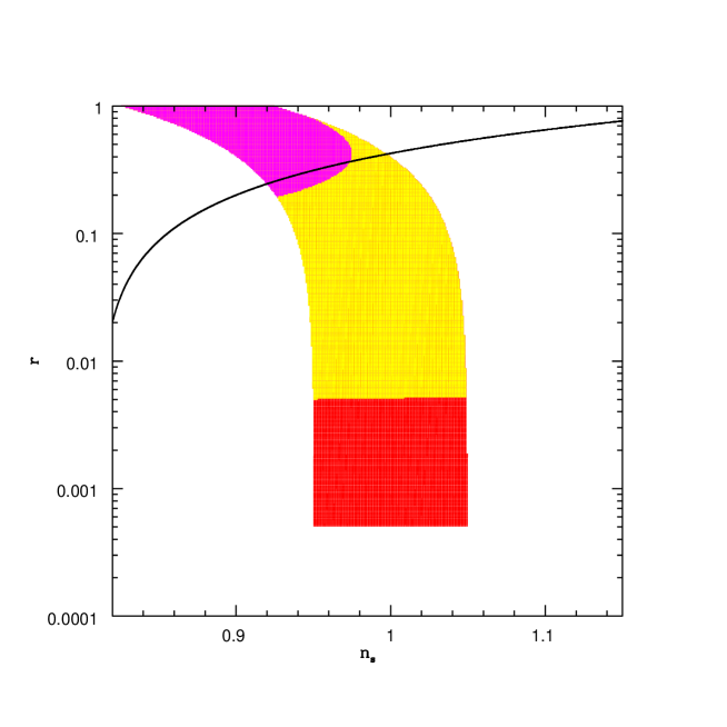
Figure 1: The sensitivity of the Big-Bang-Observer mission to a cosmic gravitational wave background generated by a single field slow-roll inflationary model. The plot shows the region in the parameter space $r$ and $n_{s}$ (see Section 2) that can be detected (corresponding to a false alarm alarm probability of $1\%$ and false dismissal rate of $10\%$). The magenta, yellow and red regions correspond to the limits obtained in a 3 yr long observation with BBO-lite, BBO-standard, and BBO-grand, respectively. The solid line correspond to the present best upperlimit set by WMAP observations [23]

On the other hand the BBO-standard configuration is able to probe the entire range of $n_{s}$ and to reach values of the scalar-to-tensor ratio $r\approx 5\times 10^{-3}$ for a 1% false alarm and 10% false dismissal rate; by adopting the BBO-grand configuration it would be possible to do even better and reach $r\approx 5\times 10^{-4}$. Notice that for $r\ll 1$, the minimum value of the scalar-to-tensor ratio $r_{\mathrm{min}}$ that can be observed scales as $r_{\mathrm{min}}\sim 1/S_{h}$, every other parameter being equal. Not surprisingly a dedicated mission such as BBO would improve our ability of probing the range of unknown parameters by (roughly) three orders of magnitudes, with respect to current limits. However, CMB experiments such as Planck (2007) and, in the more distant future, CMBPol will also be in a position of searching for the signature of a CGWB and it is worth comparing the sensitivity that can be achieved by means of indirect observations with the BBO results.

In order to make this comparison, we have determined the theoretical confidence intervals on the parameters $n_{s}$ and $r$ by computing the corresponding Fisher information matrix for Planck and CMBPol, including both the polarisation and the temperature anisotropy CMB spectra. More in detail, we have assumed as cosmology the best-fit model consistent with WMAP data [21] and we have marginalised with respect the ionisation optical depth in order to take into account its effect on the B-mode polarisation. For Planck, we have assumed an average pixel sensitivity of $11.6\,\mu$K and $24.3\,\mu$K for the temperature and polarisation anisotropies respectively, while for CMBPol the corresponding noise levels are reduced by a factor 40. Figure 2 summarises the results: we show the regions in the two-dimensional parameter space $(n_{s},r)$ corresponding to the 68% and 95% confidence level for the null hypothesis (i.e. no CGWB) for Planck and CMBPol and compare it with the limit of BBO and BBO-grand observations, respectively (those reported in Figure 1).

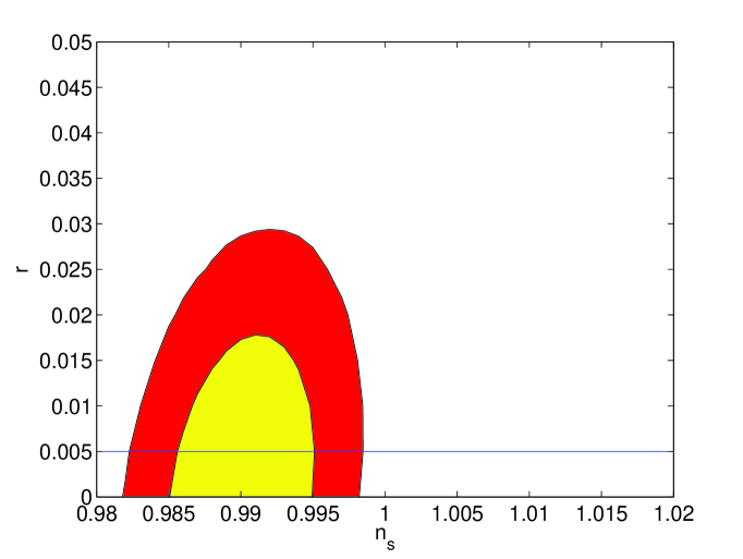
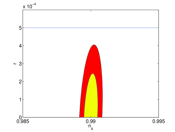
Figure 2: The sensitivity of Planck and CMBPol to indirect observations of a cosmic gravitational wave background produced during inflation. The plots show the region of the the parameter space $r$ and $n_{s}$ corresponding to the 68% and 95% confidence level upper-limit to a CGWB (red and yellow areas, respectively). The left plot corresponds to Planck observations and the line refers to the detection limit obtained with the BBO-standard configuration, cf Figure 1. The plot on the right corresponds to CMBPol observations and the line refers to the detection limit obtained with the BBO-grand configuration, cf Figure 1.

One important caveat is that the results that we have presented so far, both for direct and indirect observations, are computed assuming that the only factor limiting the sensitivity of the instruments is the intrinsic noise of the detectors, whereas other effects could actually provide the limitation. Astrophysical foregrounds and radiation from individual GW sources can limit the sensitivity of BBO. Stochastic foregrounds are produced by the incoherent superposition of radiation from large populations of astrophysical sources. Foregrounds are particularly dangerous, because they provide a fundamental sensitivity limit for the mission [10]. In the BBO band, the strongest contributions, according to our present astrophysical understanding come from rotating neutron stars and supernovae generated by population III objects[25]. Foregrounds from rotating neutron stars should not be a serious limitation, as their contribution to the spectrum is $\Omega_{\mathrm{gw}}\lower 2.15277pt\hbox{$\;\buildrel<\over{\sim}\;$}10^{-22}$. On the other hand supernovae from population III objects could be a very serious obstacle to achieve high sensitivity and might overwhelm the signal produced by inflation. In fact they could produce a foreground with intensity $h_{0}^{2}\Omega_{\mathrm{gw}}\sim 10^{-18}$ at $f\sim 1$ Hz. For comparison this is equivalent to a CGWB with $r\sim 10^{-3}$. Even assuming that no foreground is sufficiently strong to compete with the signal from inflation, deterministic signals, primarily from binary neutron stars up to high redshift, will be present in the data set and need to be identified and removed to a high degree of precision in order not to introduce spurious effects.

On the other hand the sensitivity of CMB experiments to primordial gravitational waves strongly depends on the distinctive signature produced by a CGWB on the B-mode of the CMB polarisation. Indeed the B-mode polarisation is a particular sensitive probe of primordial tensor perturbations, since it does not receive contributions from primordial density perturbations. However, gravitational lensing by cosmological structure also generates a B-mode component in the CMB polarisation  [24] and such foreground cannot be fully subtracted. The lensing contamination poses a fundamental limit on the sensitivity to a B-mode component due to primordial gravitational waves, corresponding to a lower limit on the scalar-to-tensor ratio $r$ of about $6\times 10^{-4}$ [26, 27].

4 Conclusions

The direct detection of a cosmological gravitational wave stochastic background produced during inflation is of great importance for the understanding of early Universe cosmology and shall provide a direct test of one of the fundamental, and not yet probed predictions of inflationary theories. In this paper we have explored the sensitivity of the Big-Bang-Observer mission to backgrounds generated by slow-roll, single field inflationary models and compared it with indirect limits that future CMB missions, such as Planck and CMBPol are expected to set. Our analysis shows that mild technological improvements considered for the BBO-lite configuration would not meet the science goals of a dedicated gravitational wave interferometric mission; on the other hand the ambitious choices of the instrumental parameters for the standard and grand configuration of BBO would allow us to achieve a sensitivity $h_{0}^{2}\Omega_{\mathrm{gw}}\sim 10^{-19}$ in the frequency band $0.1\,\mathrm{Hz}-1\,\mathrm{Hz}$. This value is broadly comparable with what could be achieved by one of the inflationary probes for CMB observations, such as CMBPol that are currently being discussed.

It is however important to stress that throughout this paper we have assumed that the effect of foreground emission from unresolved sources and/or lensing would have a negligible impact on the sensitivity of the missions. This hypothesis is useful to gain an insight into the ultimate performance of the experiments, but its range of validity needs to be careful investigated. For direct gravitational wave observations it is clear that at some point astrophysical foregrounds will provide the fundamental sensitivity limit. What is the level at which this can occur and the consequences on our ability of testing prediction needs to be parametrised as a function of our (still poor) knowledge of the relevant astrophysical scenarios.

References

References

- [1] A. H. Guth, Phys Rev. D 23, 347 (1981).
- [2] A. D. Linde, Phys. Lett. B 108, 389 (1982)
- [3] A. Albrecht and P. J. Steinhardt, Phys. Rev. Lett. 48, 1220 (1992).
- [4] C.L. Bennett et al., Astrophys. J. Suppl. 148, 1 (2003).
- [5] Michael S. Turner, Phys. Rev. D 55, 435 (1997).
- [6] C. Cutler and K. S. Thorne, An Overview of Gravitational-Wave Sources, Proceedings of GR16 (Durban, South Africa, 2001), gr-qc/0204090.
- [7] P. L. Bender et al., LISA Pre-Phase A Report; Second Edition, MPQ 233 (1998).
- [8] D. Hils, P. L. Bender, and R. F. Webbink, Ap. J. 360, 75 (1990).
- [9] A. J. Farmer and E. S. Phinney, Mon.Not.Roy.Astron.Soc. 346, 1197 (2003).
- [10] C. Ungarelli and A. Vecchio, Phys. Rev. D 63, 064030, (2001).
- [11] S. Phinney et al, The Big Bang Observer: Direct detection of gravitational waves from the birth of the Universe to the Present, NASA Mission Concept Study.
- [12] N. Seto, S. Kawamura and T. Nakamura, Phys. Rev. Lett. 87, 221103 (2001).
- [13] U. Seljak and M. Zaldarriaga, Phys. Rev. Lett. 78, 2054 (1997).
- [14] http://astro.estec.esa.nl/Planck/
- [15] http://universe.nasa.gov/program/inflation.html
- [16] A. Cooray, astro-ph/0503118.
- [17] K. Sigurdson and A. Cooray, astro-ph/0502549.
- [18] A.R. Liddle and D.H. Lyth, Cosmological Inflation and Large-Scale Structure, Cambridge University Press, Cambridge, (2000).
- [19] J. E. Lidsey, A. R. Liddle, E. W. Kolb, E. J. Copeland, T. Barreiro and M. Abney,Rev. Mod. Phys. 69, 373 (1997).
- [20] B. Allen and J.D. Romano, Phys. Rev. D 59, 102001 (1999).
- [21] D. N. Spergel et al., Astrophys. J. Suppl. 148, 175 (2003).
- [22] http://www.srl.caltech.edu/shane/sensitivity/
- [23] W. H. Kinney, E. W. Kolb, A. Melchiorri and A. Riotto, Phys. Rev. D 69, 103516 (2004).
- [24] M. Zaldarriaga and U. Seljak, Phys. Rev. D 58, 023003 (1998).
- [25] A. Buonanno et al., astro-ph/0412277.
- [26] L. Knox and Y. S. Song, Phys. Rev. Lett. 89, 011303 (2002).
- [27] M. Kesden, A. Cooray and M. Kamionkowski, Phys. Rev. Lett 89, 011304 (2002).