Phase-space mixing and the merging of cusps

Abstract

Collisionless stellar systems are driven towards equilibrium by mixing of phase-space elements. I show that the excess-mass function $D(f)=\int_{\bar{F}(\mn@boldsymbol{x},\mn@boldsymbol{v})>f}(\bar{F}(\mn@boldsymbol{x},\mn@boldsymbol{v})-f)\,{\mathrm{d}}^{3}\!\mn@boldsymbol{x}{\mathrm{d}}^{3}\!\mn@boldsymbol{v}$ (with $\bar{F}(\mn@boldsymbol{x},\mn@boldsymbol{v})$ the coarse-grained distribution function) always decreases on mixing. $D(f)$ gives the excess mass from values of $\bar{F}(\mn@boldsymbol{x},\mn@boldsymbol{v})>f$. This novel form of the mixing theorem extends the maximum phase-space density argument to all values of $f$. The excess-mass function can be computed from $N$-body simulations and is additive: the excess mass of a combination of non-overlapping systems is the sum of their individual $D(f)$. I propose a novel interpretation for the coarse-grained distribution function, which avoids conceptual problems with the mixing theorem.

As an example application, I show that for self-gravitating cusps ($\rho\propto r^{-\gamma}$ as $r\to 0$) the excess mass $D\propto f^{-2(3-\gamma)/(6-\gamma)}$ as $f\to\infty$, i.e. steeper cusps are less mixed than shallower ones, independent of the shape of surfaces of constant density or details of the distribution function (e.g. anisotropy). This property, together with the additivity of $D(f)$ and the mixing theorem, implies that a merger remnant cannot have a cusp steeper than the steepest of its progenitors. Furthermore, I argue that the remnant’s cusp should not be shallower either, implying that the steepest cusp always survives.

1 Introduction

The dynamical state of a stellar system is completely described by its ‘fine grained’ distribution function, $F(\mn@boldsymbol{x},\mn@boldsymbol{v},t)$, which refers to the phase-space density at point $(\mn@boldsymbol{x},\mn@boldsymbol{v})$ and time $t$. The time evolution of the distribution function is governed by a continuity equation, known as the Vlasov or collisionless Boltzmann equation,

$${\mathrm{d}}_{t}F=\partial_{t}F+\mn@boldsymbol{v}\cdot\partial_{\mn@boldsymbol{x}}F-\partial_{\mn@boldsymbol{x}}\Phi\cdot\partial_{\mn@boldsymbol{v}}F=0.$$ (1)

Here, $\Phi(\mn@boldsymbol{x})$ denotes the gravitational potential, which for a self-gravitating stellar system is given by the Poisson integral

$$\Phi(\mn@boldsymbol{x},t)=-G\int\frac{F(\mn@boldsymbol{x}^{\prime},\mn@boldsymbol{v},t)}{|\mn@boldsymbol{x}-\mn@boldsymbol{x}^{\prime}|}{\mathrm{d}}^{3}\!\mn@boldsymbol{x}^{\prime}\,{\mathrm{d}}^{3}\!\mn@boldsymbol{v}.$$ (2)

The main objective of galactic dynamics is to solve this system of equations. This is a difficult task and most analytic work is restricted to stationary or near-stationary solutions. For these a number of theoretical concepts have been developed, such as Jeans’ theorem and perturbation theory. Galactic dynamics far from equilibrium on the other hand, such as in a galaxy merger or collapse, are almost entirely treated with $N$-body simulations, i.e. numerical solutions of equations (1) and (2).

As emphasised already by Hénon (1964) and Lynden-Bell (1967), the constancy of $F(\mn@boldsymbol{x},\mn@boldsymbol{v},t)$ ensured by the collisionless Boltzmann equation (1) is of little practical use in non-equilibrium situations, because of mixing. Phase-space elements of high density are stretched out and folded with elements of low density, very much as cream stirred into coffee. As for this example, the elements become ever thinner until any measurement of $F(\mn@boldsymbol{x},\mn@boldsymbol{v},t)$ becomes impossible. In other words, the finite resolution of the system breaks the validity of the continuum limit. In such a case, the system is better described by a local average of $F$, known as the coarse-grained distribution function $\bar{F}(\mn@boldsymbol{x},\mn@boldsymbol{v},t)$. In fact, any measurement can only (hope to) recover this local average.

There are important differences between mixing in a collisionless system such as a galaxy, and a collisional system such as a gas, where mixing is driven by short-range interactions. In galaxies, strong forms of mixing are caused by non-local large-scale dynamics and occur only away from equilibrium but generally promote equilibrium. Hence, mixing is never complete in the sense of convergence to a maximum-entropy state – in fact, it can be shown that such a state does not exist (Tremaine, Henon & Lynden-Bell, 1986). A mild version of mixing is phase-mixing or similar ‘weak mixing’ processes, caused by secular evolution of stellar systems (for instance, the merging of regular orbits into a sea of chaos mixes their phase-space densities (Merritt & Valluri, 1996)). Stronger forms of mixing are ‘chaotic mixing’ or ‘violent relaxation’, which is driven by large-scale fluctuations of the gravitational potential.

Figure 1: Demonstration of phase mixing. Shown is the evolution of a bunch of $\sim 10^{5}$ phase-space points in the 1D Hamiltonian $H=p^{2}/2+|q|$ of a point mass in 1D gravity. The fine-grained distribution function is either equal to one (black) or zero (white), but at late times, a smooth distribution appears.

A simple example of mixing is presented in Figure 1: volumes of $F=1$ (black) get stretched out (e.g. at $t=100$) and folded together with volumes of $F=0$ (white) until any distinction is barred by the finite resolution of any observation. So, while at $t\ga 1000$ in this example the fine-grained distribution function $F(\mn@boldsymbol{x},\mn@boldsymbol{v},t)$ displays a very complex pattern, equilibrium is reached in the coarse-grained sense, since $\partial_{t}\bar{F}=0$.

Unfortunately, $\bar{F}$ does not obey a simple continuity equation, such as (1), and hence describing its evolution is a considerable problem. Lynden-Bell (1967) derived a distribution function for the end-state of violent relaxation assuming the conservation of phase-space volumes of given density according to equation (1). However, mixing does not conserve volumes of fixed density in the coarse-grained sense (e.g. Mathur, 1988) and, not surprisingly, the resulting theory is inconsistent (Arad & Lynden-Bell, 2005). A similar attempt by Nakamura (2000) suffers from the same deficiency (Arad & Lynden-Bell, 2005). Another approach to the dynamics of violent relaxation was taken by Chavanis (1998) in deriving a time evolution equation for $\bar{F}$. While this is a promising attempt, its practicality is limited and unlikely to surpass that of $N$-body simulations.

An obvious constraint on the evolution of $\bar{F}(\mn@boldsymbol{x},\mn@boldsymbol{v},t)$ is that its maximum value $\bar{F}_{\mathrm{max}}$ cannot increase. While this is applicable only if $\bar{F}(\mn@boldsymbol{x},\mn@boldsymbol{v})$ is initially bounded, a much stronger constraint on $\bar{F}(\mn@boldsymbol{x},\mn@boldsymbol{v},t)$ is provided by a mixing theorem, a relation between the properties of $\bar{F}(\mn@boldsymbol{x},\mn@boldsymbol{v})$ before and after a mixing process. Tremaine, Henon & Lynden-Bell (1986) considered $H$-functionals of $\bar{F}(\mn@boldsymbol{x},\mn@boldsymbol{v},t)$, which are defined as

$$H[\bar{F}]=-\int C\left(\bar{F}(\mn@boldsymbol{x},\mn@boldsymbol{v})\right)\,{\mathrm{d}}^{3}\!\mn@boldsymbol{x}\,{\mathrm{d}}^{3}\!\mn@boldsymbol{v}$$ (3)

where $C$ is a convex function with $C(0)=0$. Tremaine et al. (see also Tolman, 1938) showed that coarse-graining always increases $H$-functionals and concluded that mixing generally results in an increase of $H[\bar{F}]$, a result known as the ‘$H$-theorem’.

According to Tremaine et al. (1986), a function $\bar{F}_{2}$ is called more mixed than $\bar{F}_{1}$, if for all $H$-functionals $H[\bar{F}_{2}]\geq H[\bar{F}_{1}]$. In particular, if $\bar{F}_{2}$ originates from $\bar{F}_{1}$ by mixing, $\bar{F}_{2}$ is more mixed than $\bar{F}_{1}$. The $H$-functional for $C(f)=f\ln f$ is equal to ($k_{\mathrm{B}}$ times) the entropy and even increases for collisional systems. Tremaine et al. prove a mixing theorem stating that $\bar{F}_{2}$ is more mixed than $\bar{F}_{1}$ if and only if $\mathcal{M}_{2}(V)\leq\mathcal{M}_{1}(V)$ for all $V$, where the function $\mathcal{M}(V)$ is defined in terms of the cumulative volume and mass

$$V(f) \equiv \int_{\bar{F}(\mn@boldsymbol{x},\mn@boldsymbol{v})>f}{\mathrm{d}}^{3}\!\mn@boldsymbol{x}\,{\mathrm{d}}^{3}\!\mn@boldsymbol{v}$$ (4)

$$M(f) \equiv \int_{\bar{F}(\mn@boldsymbol{x},\mn@boldsymbol{v})>f}\bar{F}(\mn@boldsymbol{x},\mn@boldsymbol{v})\,{\mathrm{d}}^{3}\!\mn@boldsymbol{x}\,{\mathrm{d}}^{3}\!\mn@boldsymbol{v}\,$$ (5)

via $\mathcal{M}(V(f))\equiv M(f)$. This is a stronger statement than that of the increase of entropy, since it holds for all values of $V$. Unfortunately, the usability of this theorem is restricted by the complicated definition of $\mathcal{M}(V)$, which evades a simple interpretation and manipulation. For instance, $\mathcal{M}(V)$ is not additive and, if $V(f)$ is not invertible, it is not well defined, as is the case for the initial state of the example in Fig. 1, where $V=1$ for $f\leq 1$ and $V=0$ for $f>1$ (known as the ‘water-bag model’).

The purpose of this paper is to present in section 2 a novel approach to mixing which is conceptually different from that of Tremaine et al. and avoids their conceptual problems. This leads to a novel form of the mixing theorem in terms of a new concept, the excess-mass function, which is simple to apply and easy to interprete. I discuss the relation to Tremaine et al.’s work and the controversy about it in section 3. In section 4, simple examples are given and the asymptotic behaviour at small and large values of $\bar{F}$ corresponding, respectively, to large and small radii are considered. These are applied in section 5 to the merging of cusped galaxies. Finally, section 6 discusses the applicability to $N$-body simulations and section 7 concludes.

2 Mixing

In order to simplify the following discussion, it is worth introducing the ‘volume distribution function’ (e.g. Tremaine et al., 1986)

$$v(f)=\int\delta\left(\bar{F}(\mn@boldsymbol{x},\mn@boldsymbol{v})-f\right)\,{\mathrm{d}}^{3}\!\mn@boldsymbol{x}\,{\mathrm{d}}^{3}\!\mn@boldsymbol{v},$$ (6)

which refers to the phase-space volume at which $\bar{F}(\mn@boldsymbol{x},\mn@boldsymbol{v})=f$. Using $v(f)$, we can re-write the cumulative mass and volume and any $H$-functional as

$$V(f) = \phantom{-}\int_{f}^{\infty}v(\phi)\,{\mathrm{d}}\phi,$$ (7)

$$M(f) = \phantom{-}\int_{f}^{\infty}\phi\,v(\phi)\,{\mathrm{d}}\phi,$$ (8)

$$H[\bar{F}] = -\int_{0}^{\infty}v(\phi)\,C(\phi)\,{\mathrm{d}}\phi.$$ (9)

Note that $v(f)$, $V(f)$, $M(f)$, and $\mathcal{M}(V)$ are functionals of $\bar{F}(\mn@boldsymbol{x},\mn@boldsymbol{v})$ as well as functions of their parameter $f$ or $V$. We can now model mixing directly as an operation on phase-space volumes.

2.1 Infinitesimal mixing events

The process of mixing and subsequent coarse-graining of the distribution function can be described as sequence of infinitesimal mixing events in which a phase-space element with infinitesimal volume ${\mathrm{d}}V_{\mathrm{l}}$ and density $f_{\mathrm{l}}$ mixes completely with another volume ${\mathrm{d}}V_{\mathrm{h}}$ having density $f_{\mathrm{h}}\geq f_{\mathrm{l}}$. Because of conservation of mass and of phase-space volume, the resulting element has volume ${\mathrm{d}}V_{\mathrm{l}}+{\mathrm{d}}V_{\mathrm{h}}$ and density

$$f_{\mathrm{m}}=\frac{{\mathrm{d}}V_{\mathrm{l}}\,f_{\mathrm{l}}+{\mathrm{d}}V_{\mathrm{h}}\,f_{\mathrm{h}}}{{\mathrm{d}}V_{\mathrm{l}}+{\mathrm{d}}V_{\mathrm{h}}}$$ (10)

(Mathur, 1988). The change in the volume distribution function due to such an event is

$${\mathrm{d}}v(f)=({\mathrm{d}}V_{\mathrm{l}}+{\mathrm{d}}V_{\mathrm{h}})\,\delta(f-f_{\mathrm{m}})-{\mathrm{d}}V_{\mathrm{l}}\,\delta(f-f_{\mathrm{l}})-{\mathrm{d}}V_{\mathrm{h}}\,\delta(f-f_{\mathrm{h}})$$ (11)

Mixing events with $f_{\mathrm{l}}=f_{\mathrm{h}}$ do not affect $v(f)$ and hence may be called ‘adiabatic’.

Figure 2: In a plot of cumulative volume $V(\phi)$ vs. phase-space density $\phi$, the excess-mass $D(f)$ is given by the horizontally shaded region (equation 14), which equals $M(f)$ (total shaded region) minus $fV(f)$ (vertically shaded; equation 15).

2.2 A lemma on mixing

Consider the following function

$$D(f)\equiv\int\limits_{\bar{F}(\mn@boldsymbol{x},\mn@boldsymbol{v})>f}\left(\bar{F}(\mn@boldsymbol{x},\mn@boldsymbol{v})-f\right)\,{\mathrm{d}}^{3}\!\mn@boldsymbol{x}\,{\mathrm{d}}^{3}\!\mn@boldsymbol{v},$$ (12)

which may be re-written as

$$D(f) = \int_{f}^{\infty}(\phi-f)\,v(\phi)\,{\mathrm{d}}\phi$$ (13)

$$= \int_{f}^{\infty}V(\phi)\,{\mathrm{d}}\phi,$$ (14)

$$= M(f)-f\,V(f).$$ (15)

As is obvious from these relations, the excess-mass function $D(f)$ refers to the excess mass due to values of $\bar{F}>f$ (see also Fig. 2).

Mixing lemma.

Mixing of phase-space volumes where $\bar{F}(\mn@boldsymbol{x},\mn@boldsymbol{v})<f$ with volumes where $\bar{F}(\mn@boldsymbol{x},\mn@boldsymbol{v})>f$ decreases $D(f)$; other mixing processes leave $D(f)$ unchanged.

Proof: First, consider an infinitesimal mixing event. The changes it imposes on $D(f)$ are easily found from equations (11) and (13):

$${\mathrm{d}}D(f)=\left\{\begin{array}[]{l@{\hspace{4mm}}l@{\hspace{4mm}}lllll}0\hfil\hskip 11.38109pt&\mbox{for}\hfil\hskip 11.38109pt&&&f&<&f_{\mathrm{l}},\\ -(f-f_{\mathrm{l}})\,{\mathrm{d}}V_{\mathrm{l}}\hfil\hskip 11.38109pt&\mbox{for}\hfil\hskip 11.38109pt&f_{\mathrm{l}}&<&f&<&f_{\mathrm{m}},\\ -(f_{\mathrm{h}}-f)\,{\mathrm{d}}V_{\mathrm{h}}\hfil\hskip 11.38109pt&\mbox{for}\hfil\hskip 11.38109pt&f_{\mathrm{m}}&\leq&f&<&f_{\mathrm{h}},\\ 0\hfil\hskip 11.38109pt&\mbox{for}\hfil\hskip 11.38109pt&f_{\mathrm{h}}&<&f.\end{array}\right.$$ (16)

Thus, ${\mathrm{d}}D(f)<0$ for $f_{\mathrm{l}}<f<f_{\mathrm{h}}$ and 0 otherwise. Since the whole mixing process is a sequence of infinitesimal mixing events, the change in $D(f)$ is the integral over many infinitesimal changes ${\mathrm{d}}D(f)$ and the lemma follows.

The largest change of $D(f)$ due to an infinitesimal mixing event occurs at $f{=}f_{\mathrm{m}}$ and is ${\mathrm{d}}D(f_{\mathrm{m}})=-|f_{\mathrm{h}}-f_{\mathrm{l}}|{\mathrm{d}}V_{\mathrm{l}}\,{\mathrm{d}}V_{\mathrm{h}}/({\mathrm{d}}V_{\mathrm{l}}+{\mathrm{d}}V_{\mathrm{h}})$.

2.3 Further properties of the excess-mass function

Apart from the relations (13), (15), and (14), the function $D(f)$ has the following properties. First,

$$D^{\prime}(f) = -V(f),$$ (17)

$$D^{\prime\prime}(f) = \phantom{-}v(f).$$ (18)

Since both $v(f)$ and $V(f)$ are non-negative, this implies that $D(f)$ is non-negative and monotonically declining with everywhere non-negative curvature.

Second, since in order for $M(f\to\infty)$ not to diverge $f^{2}v(f)\to 0$ as $f\to\infty$, and because of equation (18),

$$\lim_{f\to\infty}D(f)=0.$$ (19)

Third, for a system with finite mass,

$$D(0)=M_{\mathrm{total}}.$$ (20)

Fourth, changes in $D(f)$ are related to a change of the entropy $S$ via

$$\Delta S=-k_{\mathrm{B}}\int_{0}^{\infty}\frac{\Delta D(f)}{f}\,{\mathrm{d}}f,$$ (21)

which becomes obvious at the end of the next section.

Finally, the combined excess-mass function of several disjoint systems (whose distribution functions do not overlap) is simply given by the sum of the individual excess-mass functions. In general, i.e. for partially overlapping systems, the excess-mass function is super-additive:

$$D_{1+2}(f)\geq D_{1}(f)+D_{2}(f).$$ (22)

This is directly related to the sub-additivity of the entropy (e.g. Wehrl, 1978) and follows from the definition (12) of $D(f)$ and the fact that $\bar{F}_{1+2}=\bar{F}_{1}+\bar{F}_{2}$.

2.4 A mixing theorem

The above lemma is closely related to a statement made by Mathur (1988). In fact, his function $P(f)$, for which he only gives the second derivative, is identical to the change in $D(f)$ induced by mixing and his equation (7) is equivalent to my (16).

The relation to the theorem given by Tremaine et al. (1986) and outlined in the beginning of this section is more subtle. In the proof of their theorem, Tremaine et al. construct the function $D(f)$, because it actually is (the negative of) an $H$-functional of $\bar{F}$. In fact, as pointed out by Mathur (1988), $D(f)$ and $\mathcal{M}(V)$ are related by a Legendre transformation, as is obvious from equation (15). In particular, $\mathcal{M}^{\prime}(V)=f$, $\mathcal{M}^{\prime\prime}(V)=1/v(f)$, and $D^{\prime}$ (equation 17) is the (negative of the) inverse of $\mathcal{M}^{\prime}$, by definition of a Legendre transform. This is directly related to the fact that

$$\left(\frac{\partial D}{\partial\tau}\right)_{f}=\left(\frac{\partial\mathcal{M}}{\partial\tau}\right)_{V}$$ (23)

where $\tau$ is a time-like variable describing the evolution due to mixing. Equation (23) in conjunction with the theorem given by Tremaine et al. (1986) implies the following alternative form of the mixing theorem.

Mixing theorem.

The distribution function $\bar{F}_{2}(\mn@boldsymbol{x},\mn@boldsymbol{v})$ is more mixed than $\bar{F}_{1}(\mn@boldsymbol{x},\mn@boldsymbol{v})$ if and only if $D_{2}(f)\leq D_{1}(f)$ for all $f$.

Proof: Suppose $\bar{F}_{2}$ is more mixed than $\bar{F}_{1}$. Then $D_{2}(f)\leq D_{1}(f)$, since $D(f)$ is the negative of a $H$-functional of $\bar{F}(\mn@boldsymbol{x},\mn@boldsymbol{v})$ with the convex function

$$C(\bar{F})=\left\{\begin{array}[]{l@{\hspace{4mm}}l}0\hfil\hskip 11.38109pt&\mbox{for $\quad\bar{F}\leq f$},\\ \bar{F}-f\hfil\hskip 11.38109pt&\mbox{for $\quad\bar{F}>f$}.\end{array}\right.$$ (24)

Conversely, suppose $D_{2}(f)\leq D_{1}(f)$ for all $f$. From equation (9),

$$H_{2}-H_{1}=-\int_{0}^{\infty}(v_{2}-v_{1})C\,{\mathrm{d}}f.$$ (25)

Integrating by parts and using $V^{\prime}=-v$ yields

$$H_{2}-H_{1}=(V_{2}-V_{1})C\Big{|}_{0}^{\infty}-\int_{0}^{\infty}(V_{2}-V_{1})C^{\prime}\,{\mathrm{d}}f.$$ (26)

The first term on the right-hand side vanishes, and integrating the second term by parts using (17) gives

$$H_{2}-H_{1}=(D_{2}-D_{1})C^{\prime}\Big{|}_{0}^{\infty}-\int_{0}^{\infty}(D_{2}-D_{1})C^{\prime\prime}\,{\mathrm{d}}f.$$ (27)

Again the first term on the right-hand side vanishes; the second term is non-negative, since $D_{2}\leq D_{1}$ by assumption and $C^{\prime\prime}\geq 0$ by definition of convexity. Hence $H_{2}\geq H_{1}$, which completes the proof.

Together with the above lemma, this theorem is another proof of the $H$-theorem (mixing increases or preserves but never decreases any $H$-functional).

Since the entropy $S$ is the $H$-functional with $C(f)=f\ln f$, the relation (21) between changes in entropy and $D(f)$ follows directly from equation (27).

2.5 Diluting phase-space density

The theorem above is more useful than the equivalent theorem by Tremaine et al. (1986) because the function $D(f)$ is easier to comprehend and manipulate than $\mathcal{M}(V)$. In particular the additivity of $D(f)$ is of great value. However, the lemma of §2.2 is of even larger practical significance, because it allows us to relate the change in $D(f)$ directly to mixing events ‘across’ $\bar{F}=f$.

The total change of $D(f)$ in a mixing process may be obtained by integrating the infinitesimal change (16) over a function which specifies for each pair $(f_{\mathrm{l}},f_{\mathrm{h}})$ how much phase space at $f_{\mathrm{l}}$ mixes with how much phase space at $f_{\mathrm{h}}$ (Mathur, 1988). However, it is not clear how such a function may be obtained; moreover, in the end the information contained in this function is reduced to the one-dimensional change in $D(f)$. One may instead assume a simple form for this function, resulting in simple mixing models

For instance, one may assume that all of $v(f)$ gets mixed with an empty volume of size $\alpha(f)v(f)$. This complete ‘mixing with air’ simply dilutes the phase-space density $\bar{F}\to\bar{F}/[1+\alpha(\bar{F})]$ and gives

$$D_{\mathrm{final}}(f)=D_{\mathrm{initial}}([1+\alpha(f)]f).$$ (28)

The dilution function $\alpha(f)$ is always well-defined and can be measured directly from $N$-body experiments, by estimating $D(f)$ before and after a violent mixing process. Essentially $\alpha(f)$ gives the equivalent amount of mixing with air necessary to generate a certain evolution of $D(f)$.

3 Coarse-Graining

3.1 Conceptual problems

As mentioned in footnote 2 above, the $H$-theorem of Tremaine et al. (1986) has met immediate rejection (Dejonghe, 1987; Kandrup, 1987; Sridhar, 1987). These authors provided simple counter-examples of non-mixing systems whose $H$-functionals are not conserved or even decreasing and pointed to the following conceptual problem in the argumentation. Tremaine et al. have actually only proven that $H$-functionals increase as consequence of coarse-graining: $H[\bar{F}(\mn@boldsymbol{x},\mn@boldsymbol{v})]\geq H[F(\mn@boldsymbol{x},\mn@boldsymbol{v})]$ independent of the actual dynamics or indeed mixing. From that, they argued that initially $\bar{F}=F$ (which can be guaranteed by definition of the arrow of time, Tremaine, private communication), but $\bar{F}\neq F$ at a later time $t$, and hence $H[\bar{F}(0)]\leq H[\bar{F}(t)]$. However, this argument does not guarantee that $H[\bar{F}(0)]\leq H[\bar{F}(t_{1})]\leq H[\bar{F}(t)]$ at intermediate times $t_{1}$.

Unfortunately, this controversy undermined the whole subject of mixing in stellar dynamics. Some sceptics argue that the fine-grained distribution function never suffers information loss and hence that the $H$-theorem is a pure artifact of coarse-graining (implying that the entropy of a collisionless stellar system is constant). This argument, however, relies on the infinite resolution of the fine-grained distribution function and ignores the fact that no stellar system can support infinite resolution. The fine-grained distribution function and the CBE only give an approximative description of collisionless stellar dynamics (e.g. Dejonghe, 1987). In the presence of mixing, the continuum limit, on which this approximation rests, becomes invalid. Mixing is an irreversible process as information about the state prior to mixing is lost, representing a true entropy increase in the sense understood by Boltzmann (Merritt, 1999).

The conceptual problems related to the $H$-theorem originate from the fact that the details of and requirements for the coarse-graining operation are not specified and hence are usually considered unimportant. Many authors consider a static coarse-graining operation, such as averaging over time-independent macro cells or convolution with a window function. For such ways of coarse-graining Soker (1996) showed that $H[\bar{F}]$ does not obey a $H$-theorem. The reason is easily understood when considering a non-mixing non-equilibrium (e.g. periodic) system. Since the system evolves, the effectively resolved mass per fixed macro cell evolves too, so that $H[\bar{F}]$ is not necessarily conserved.

3.2 A novel interpretation of coarse-graining

In this situation, it is instructive to consider the proof of the $H$-theorem from the previous section. Unlike Tremaine et al.’s proof, it does not employ coarse-graining with finite macro cells. Rather mixing is described directly as (integral over) averaging of infinitesimal phase-space volumes. In this description, the astrophysical process of mixing (and the resulting loss of information) is accounted for, in our description of the system, by a local averaging, the coarse-graining. Thus, mixing and coarse-graining are intimately related and the latter must not be considered arbitrary.

This is directly related to the interpretation of the coarse-grained distribution function $\bar{F}$. Traditionally, $\bar{F}$ is introduced, because its fine-grained pendant $F$ does not tend to equilibrium, but undergoes ever stronger small-scale fluctuations (e.g. Chavanis, 1998). In this picture, $\bar{F}$ gives an otherwise unspecified, finite-resolution representation of the system. As already mentioned, the fine-grained fluctuations of $F$ will eventually break the validity of the continuum approximation, i.e. below some level, these fluctuations are artificial and not representative of the actual stellar system.

These arguments suggest the interpretation of $\bar{F}$ as our best possible description of the stellar system, avoiding the artifacts of its fine-grained counterpart. In this interpretation, coarse-graining must meet the following conditions.

1. In the limit of a system with infinite resolution: $\bar{F}\to F$.

2. $\bar{F}$ must be a faithful representation of the system.

3. In the absence of mixing: ${\mathrm{d}}_{t}\bar{F}=0$.

The first two conditions imply that coarse-graining must be local. The second condition ensures that coarse-graining only deletes information in $F$ but not in our description of the stellar system, in particular $\bar{\bar{F}}=\bar{F}$. This means that coarse-graining is done on the local resolution scale of the system itself, which seems the most natural scale to use, but excludes static coarse-graining. In particular, any moment of the stellar system must agree (within its statistical uncertainty) with the corresponding moment of $\bar{F}$. Finally, the last condition guarantees that $\bar{F}$ is altered by mixing only, i.e. under ordinary non-mixing circumstances all information about the system is preserved in $\bar{F}$. This immediately warrants the $H$-theorem.

It is not clear, whether and how these conditions can be met in a practical implementation. However, even if we could only generate an approximation to this ideal, the above conditions and the underpinning interpretation were still valuable. For instance, we would allow for an approximation error $\hat{\bar{F}}-\bar{F}$ (with $\hat{\cdot}$ denoting approximation), which in turn might result in spurious but accountable violations of the $H$-theorem. Clearly, a more detailed investigation of these issues is beyond the scope of this paper.

We should stress that the idea of $\bar{F}(\mn@boldsymbol{x},\mn@boldsymbol{v},t)$ being the best possible description of the stellar system is not necessarily consistent with other approaches. For instance, Chavanis (1998, see also Chavanis & Bouchet 2005) consider $\bar{F}$ to contain a truly reduced information and, hence, the fluctuations of $F$ to be (at least partially) real rather than entirely artificial. It may be possible to reconcile this with our ideas by altering the above conditions to allow for a arbitrary resolution (in terms of the mass or number of stars per resolution element) without spoiling the $H$-theorem – however, then ${\mathrm{d}}_{t}\bar{F}\neq 0$ because of the forces generated by the fluctuations (Chavanis, 1998).

4 Examples

4.1 Asymptotics at large $f$

Figure 3: The excess-mass function $D(f)$ for the (non-singular) isothermal sphere.

4.1.1 Density cores: limited phase-space densities

Let us consider the (non-singular) isothermal sphere (e.g., Binney & Tremaine, 1987). I have numerically obtained the potential $\Phi(r)$ as well as the phase-space volume $g(E)$ at constant energy. The volume distribution function is then given by $g(E)/|{\mathrm{d}}F/{\mathrm{d}}E|$ and $D(f)$ can be computed using equation (13). The result is plotted in Figure 3. The mass of the isothermal sphere is infinite and hence $D\to\infty$ as $f\to 0$. The maximum phase-space density is $f_{\mathrm{max}}=2\rho_{0}/[9(2\pi\sigma)^{3/2}]$, where $\sigma$ and $\rho_{0}$ denote the velocity dispersion and central density, respectively. At $f\approx f_{\mathrm{max}}$, the excess-mass function decays like $D\propto(f_{\mathrm{max}}-f)^{4}$.

4.1.2 Density cusps: unlimited phase-space densities⁵

Let us consider a self-gravitating stellar system whose density at small radii is given by a power law in radius, corresponding to a density cusp

$$\rho(\mn@boldsymbol{x})=\rho_{0}\,\varrho(\hat{\mn@boldsymbol{x}})\,x^{-\gamma}$$ (29)

with $\hat{\mn@boldsymbol{x}}\equiv\mn@boldsymbol{x}/|\mn@boldsymbol{x}|$ the unit vector in direction of $\mn@boldsymbol{x}$ and the dimensionless radius $x\equiv|\mn@boldsymbol{x}|/r_{\mathrm{u}}$, where $r_{\mathrm{u}}$ is the unit of length. The parameters $\rho_{0}$ and $0<\gamma<3$ are, respectively, a density normalisation and cusp strength. The dimensionless and continuous function $\varrho(\hat{\mn@boldsymbol{x}})$ determines the shape of surfaces of equal density. I proceed by assuming that the distribution function is of the form

$$\bar{F}=\rho_{0}v_{0}^{-3}h(\mn@boldsymbol{X})\tilde{f}(E)$$ (30)

with the constant $v_{0}$ given in equation (43). Here $E=\mn@boldsymbol{v}^{2}/2+\Phi(\mn@boldsymbol{x})$ is the energy, while $\mn@boldsymbol{X}=\mn@boldsymbol{X}(\mn@boldsymbol{x},\mn@boldsymbol{v})$ denotes a set of scale-invariant integrals of motion. Scale invariance in this case means that

$$\mn@boldsymbol{X}(\mn@boldsymbol{x},\mn@boldsymbol{v})=\mn@boldsymbol{X}(a\mn@boldsymbol{x},a^{1-\gamma/2}\mn@boldsymbol{v})$$ (31)

for any dimensionless scale factor $a$. Examples for scale-invariant properties of stellar orbits are the eccentricity and ratios between orbital frequencies or actions. After some algebra (see appendix A), the excess-mass of the self-gravitating cusp function is found to be

$$D(f)=\mathrm{D}_{\gamma h}\,r_{\mathrm{u}}^{3}\rho_{0}\,(f^{2}\,G^{3}\rho_{0}r_{\mathrm{u}}^{6})^{-\frac{3-\gamma}{6-\gamma}}.$$ (32)

Here, $\mathrm{D}_{\gamma h}$ is a dimensionless constant given in equation (54), which for the spherical ($\varrho\equiv 1$) and isotropic ($h\equiv 1$) case reduces to a simple expression (see appendix A).

The exponent in $D\propto f^{-2(3-\gamma)/(6-\gamma)}$ varies only between $1$ for $\gamma\to 0$ and 0 for $\gamma\to 3$ and decreases with increasing $\gamma$, i.e. a steeper cusp is less mixed than a shallower one. Moreover, this asymptotic behaviour of $D(f)$ depends only on the cusp strength and not on the details of the density contours or the distribution function, as long as it is scale-invariant.

For a non-self-gravitating system with density $\propto r^{-\gamma}$ immersed in a gravitational field generated by an overall mass density $\rho\propto r^{-\beta}$ with $\beta\geq\gamma$, one finds by a similar analysis

$$D\propto f^{-2(3-\gamma)/(6+2\gamma-3\beta)}.$$ (33)

4.1.3 Stellar systems dominated by a super-massive black hole

The case of a stellar system whose dynamics is dominated by a super-massive black hole corresponds to $\beta=3$ in equation (33), i.e. gives $D\propto f^{-2(3-\gamma)/(2\gamma-3)}$. Note that the phase-space density of such a system is unlimited only for $\gamma>3/2$. The exponents in this relation vary between $\infty$ for $\gamma\to 3/2$ and $0$ for $\gamma\to 3$. Thus, again steeper cusps are less mixed, but the differences are much more pronounced than for self-gravitating cusps.

4.2 Asymptotics at small $f$

Next, consider a stellar system of finite mass. For simplicity, I consider the case of spherical density only. The potential in the outer parts is dominated by the monopole, i.e. $\Phi=-GM/r$, while the density is assumed to be of the form $\rho=\rho_{0}(r/r_{\mathrm{u}})^{-\eta}$ with $\eta>3$ for the mass not to diverge at $r\to\infty$. A distribution function of the form $\bar{F}\propto L^{-2\beta}\tilde{f}(E)$ always generates a constant Binney anisotropy $\beta\equiv 1-\sigma_{\theta}^{2}/\sigma_{r}^{2}$ (Cuddeford, 1991). For the case considered here, this gives

$$\bar{F}=\rho_{0}\,(GM/r_{\mathrm{u}})^{-3/2}\,\mathrm{f}_{\eta\beta}\,X^{-\beta}\,\mathcal{E}^{\eta-3/2},$$ (34)

where $\mathcal{E}=-r_{\mathrm{u}}E/GM$, $X\equiv L^{2}/L^{2}_{\mathrm{circ}}(E)=1-\epsilon^{2}$ (orbital circularity), and $\mathrm{f}_{\eta\beta}^{-1}=2^{3/2}\pi B(\frac{1}{2},1-\beta)B(\frac{3}{2}-\beta,\eta-\frac{1}{2}-\beta)$. The phase-space volume at fixed $(E,X)$

$$g(E,X)=\sqrt{2GMr_{\mathrm{u}}^{5}}\,\pi^{3}\mathcal{E}^{-5/2}$$ (35)

is independent of $X$. From these, one can obtain $v(f)$ and

$$D(f)=M_{\mathrm{D}}-\rho_{0}r_{\mathrm{u}}^{3}\,\mathrm{D}_{\eta\beta}\,\left(\frac{f^{2}G^{3}M^{3}}{r_{\mathrm{u}}^{3}\rho_{0}^{2}}\right)^{\frac{\eta-3}{2\eta-3}}$$ (36)

with $M_{\mathrm{D}}\leq M$ the total mass of the density component considered and

$$\mathrm{D}_{\eta\beta}=\frac{2^{1/2}\,\pi^{3}(2\eta-3)^{2}}{3(\eta-3)(2\eta-3-3\beta)}\,\mathrm{f}_{\eta\beta}^{3/(2\eta-3)}.$$ (37)

Hence, again the asymptotic is independent of details like the orbital anisotropy.

Figure 4: Top: The excess-mass function $D(f)$ for spherical and isotropic $\gamma$ models, which have density $\rho\propto r^{-\gamma}(r+a)^{\gamma-4}$. The curves correspond to values of $\gamma$ from 0.25 (lowest) to 2.5 (uppermost) spaced by 0.25 with $\gamma=1$ and $\gamma=2$ plotted solid. Units correspond to $G$, $a$ and total mass equal to unity. Bottom: The same, but plotting $D/(1-D/M_{\mathrm{tot}})$, which distinguishes the models at $f\to 0$ and demonstrates that in this limit they indeed behave as equation (36) predicts for $\eta=4$.

4.3 Excess-mass functions of the $\gamma$ models

Figure 4 shows the excess-mass function of the spherical $\gamma$-models (Dehnen, 1993; Tremaine et al., 1994, with $M$ and $a$ denoting total mass and scale radius)

$$\rho=\frac{3-\gamma}{2\pi}\frac{Ma}{r^{\gamma}(r+a)^{4-\gamma}}$$ (38)

with isotropic velocity distribution. Evidently, $D_{1}<D_{2}$ for $\gamma_{1}<\gamma_{2}$, thus $\gamma$-models are less mixed with increasing $\gamma$. The bottom panel shows $D/(1-D/M_{\mathrm{tot}})$ and enables to better distinguish between the excess-mass functions at $f\to 0$. The line shows the asymptotic slope predicted by equation (36).

5 Application: merging Cusps

As application, consider the merging of several cusped galaxies or dark-matter haloes. Because of its additivity the combined $D(f)$ prior to the merger is equal to the sum of those of the progenitors. When equilibrium has been re-established after the merger, $D_{\mathrm{r}}(f)$ of the merger remnant must satisfy

$$D_{\mathrm{r}}(f)\leq D_{\Sigma}(f)\equiv\sum_{i}D_{i}(f).$$ (39)

5.1 Constraints on the cusp strength

Let us first consider the combined excess-mass function of the progenitors on the right-hand side of (39). Each $D_{i}(f)$ is of the form (32): $D_{i}\propto f^{-2(3-\gamma_{i})/(6-\gamma_{i})}$. Thus, at sufficiently large phase-space densities $D_{\Sigma}$ will be dominated by the steepest progenitor cusp. Next suppose the remnant also forms a scale-free cusp, such that its excess-mass function $D_{\mathrm{r}}\propto f^{-2(3-\gamma_{\mathrm{r}})/(6-\gamma_{\mathrm{r}})}$. Then for condition (39) to be satisfied $\gamma_{\mathrm{r}}\leq\max_{i}\{\gamma_{i}\}$. Thus, the remnant cusp cannot be steeper than any of the progenitor cusps.

In other words, steeper cusps are less mixed than shallower cusps (in the limit $f\to\infty$) regardless of details such as the shape of the density contours or the distribution of orbital shapes (orbital anisotropy), as long as these are the same for all radii and/or energies (scale freedom). This implies that by virtue of the mixing theorem mergers cannot produce cusps steeper than those already present in their progenitors. Conversely, a remnant cusp shallower than the steepest of its progenitors would require an arbitrarily large dilution $\alpha$ of the distribution function as $f\to\infty$. This, while not impossible, seems highly implausible, which strongly suggests that the remnant cusp should not be shallower than the steepest of its progenitors. Together with the above mixing constraint, this means that the maximum cusp strength is conserved when merging collisionless stellar systems.

5.2 Constraints on the cusp mass

Let me exemplify the merging of two equal and cusped galaxies a little more. I assume that the remnant has the same scale-invariant structure and cusp strength $\gamma$ as its progenitors, but different density normalisation, $\rho_{0\mathrm{r}}\neq\rho_{0\mathrm{p}}$. Under these circumstances, the dilution function $\alpha(f)$ of equation (28) is constant (in the asymptotic limit considered). Together with equation (32) and the additivity, this yields

$$\rho_{0\mathrm{r}}=\rho_{0\mathrm{p}}\,2^{-\frac{6-\gamma}{3}}\,(1+\alpha)^{-\frac{3}{2(3-\gamma)}}.$$ (40)

Thus, for $\rho_{0\mathrm{r}}=2\rho_{0\mathrm{p}}$ (i.e. the remnant cusp containing the sum of the progenitor-cusp masses), the dilution fraction has to be $\alpha=\sqrt{2}-1\approx 41\%$ independent of $\gamma$. For the remnant cusp to be equally massive as either of its progenitors, $\alpha=2^{(6-\gamma)/2(3-\gamma)}-1$, which evaluates to 1 for $\gamma=0$, to $\approx 138\%$ for $\gamma=1$, to $\approx 183\%$ for $\gamma=1.5$, and $3$ for $\gamma=2$. Thus, if $\alpha$ is not strongly dependent on $\gamma$, relation (40) suggests that remnants of steep-cusp mergers have more massive cusps, compared to their progenitors, than remnants of shallow-cusp mergers. However, since steeper cusps generate stronger tides, one would indeed expect $\alpha$ to depend on $\gamma$ in a sense opposing the above trend.

6 Application to $N$-body simulations

One of the motivations of this study was the hope to use the excess-mass function as a diagnostic tool in the interpretation and validation of $N$-body experiments. To this end it is necessary to estimate phase-space densities from $N$-body data. Arad, Dekel & Klypin (2004) and Ascasibar & Binney (2005) have demonstrated in two pioneering studies that this can in principle be done, even though it is a difficult task, because of (i) the vastness of 6D phase space and (ii) the lack of a metric.

Once estimates $\hat{\bar{F}}_{i}$ for $\bar{F}$ at the phase-space positions of the bodies have been obtained, the excess-mass function may be estimated as

$$\hat{D}(f)=\sum_{\hat{\bar{F}}_{i}>f}m_{i}-f\sum_{\hat{\bar{F}}_{i}>f}\frac{m_{i}}{\hat{\bar{F}}_{i}},$$ (41)

where $m_{i}$ denotes the mass of the $i$th body. A serious problem in this game is that the coarse-graining scale used in the estimation of $\bar{F}$ may well be larger than the scales still resolved by the system. As discussed in section 3, this approximation error may result in unwanted surprises (such as $\hat{D}$ increasing with time).

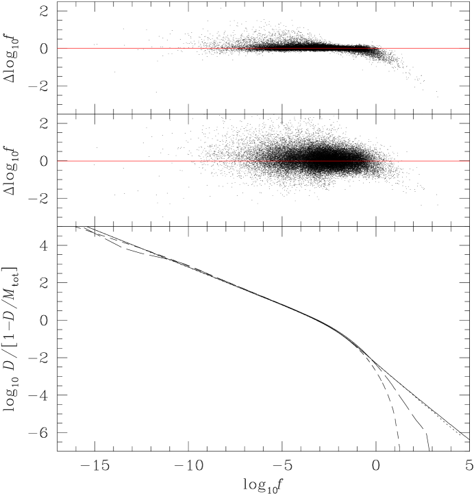
Figure 5: Assessing the fitness of FiEstAS for estimating $D(f)$. Top: error in the FiEstAS estimates $\hat{\bar{F}}_{i}$ for $\bar{F}$ from $N=10^{6}$ points drawn from a Hernquist (1990) sphere ($\gamma=1$ in Fig. 4) plotted versus their true phase-space density (only every 25th body plotted). Middle: the same, but using FiEstAS without smoothing. Bottom: Excess-mass function of the same model (solid), and estimates for $D(f)$ using equation (41) and the true fine-grained $F$ of $N=10^{6}$ points (dotted), or the FiEstAS estimates $\hat{\bar{F}}_{i}$ for the same points with (long dashed) and without smoothing (short dashed).

Figure 5 demonstrates these problems when applying the phase-space density estimator FiEstAS of Ascasibar & Binney (2005) to $10^{6}$ points drawn from a Hernquist (1990) sphere. The top two panels show that the estimated density can be up to two orders of magnitude wrong and is systematically too large for $f\la 0.01$, while high densities are truncated, in particular when smoothing is used (top panel). The bottom panel shows the estimate $\hat{D}(f)$ obtained from equation (41) and the FiEstAS estimated densities with (short dashed) and without (long dashed) smoothing. A comparison with the true $D(f)$ (solid) shows that the estimated $D(f)$ is only slightly too large at intermediate $f$, but is seriously in error at large $f$ (and also at very small $f$), in particular when smoothing was used. These errors are obviously related to the underestimation of large phase-space densities. This underestimation occurs at values for $\bar{F}$ below those expected from the finite resolution with $N=10^{6}$, since $M(f)/M_{\mathrm{tot}}=10^{-6}$ at $f\approx 10^{4.7}$ and $10^{-5}$ at $f\approx 10^{3.5}$.

Also plotted are the estimates from equation (41) using the true fine-grained phase-space densities of $10^{6}$ bodies (dotted). These can hardly be distinguished from the true $D(f)$, indicating that equation (41) gives a fairly good estimator provided the estimates $\hat{\bar{F}}_{i}$ are good.

These results suggest that, in order to resolve the asymptotic behaviour of $D(f)$ at $f\to\infty$, at least $\sim 10^{7}$ points are required with this technique. Clearly, there must be ways to improve the situation. Apart from improvements in the existing technique, one may exploit that ${\mathrm{d}}_{t}\bar{F}=0$ (assuming no mixing is going on) in order to constrain the possible values for $\hat{\bar{F}}_{i}$.

7 Summary and Conclusion

A stellar system out of equilibrium is driven towards equilibrium by way of mixing its phase-space densities in a process of violent relaxation. As a consequence the concept of the fine-grained distribution function $F(\mn@boldsymbol{x},\mn@boldsymbol{v})$ is ill-suited to understand non-equilibrium stellar dynamics. Instead, the system is better described in terms of its coarse-grained distribution function $\bar{F}(\mn@boldsymbol{x},\mn@boldsymbol{v})$. Mixing of phase-space elements changes $\bar{F}$ in such a way that the excess-mass function

$$D(f)\equiv\int\limits_{\bar{F}(\mn@boldsymbol{x},\mn@boldsymbol{v})>{f}}\left(\bar{F}(\mn@boldsymbol{x},\mn@boldsymbol{v})-{f}\right)\,{\mathrm{d}}^{3}\!\mn@boldsymbol{x}\,{\mathrm{d}}^{3}\!\mn@boldsymbol{v}$$

decreases (mixing lemma, section 2.2), equivalent to a statement by Mathur (1988). In fact, only events which mix densities $>f$ with densities $<f$ decrease $D(f)$. This lemma may be considered an extension of the well-known maximum phase-space density argument to all density values. $D(f)$ measures the excess mass due to phase-space densities higher than $f$ and its decrease is directly related to entropy increase, see equation (21). A useful property of $D(f)$ is its additivity: the excess-mass function of the combination of disjoint stellar systems (which do not overlap in phase space) is simply the sum of the individual $D(f)$.

In section 2.4, I prove a novel form of the mixing theorem (Tremaine, Henon & Lynden-Bell, 1986), stating that $D(f)$ decreases if and only if any $H$-functional of the distribution function increases. My lemma together with this theorem is an alternative proof of the $H$-theorem (the increase of $H$-functionals due to mixing), avoiding some conceptual problems associated with allowing arbitrary coarse-graining.

In section 3, the importance of details of the coarse-graining operator for the validity of the $H$-theorem are discussed. It is argued that the conceptual problems of Tremaine et al.’s proof of this theorem can be avoided by requiring appropriate coarse-graining. In particular, I propose an interpretation of the coarse-grained distribution function $\bar{F}$ as the best possible description of the stellar system. In this interpretation, the astrophysical process of mixing is directly described by coarse-graining and in the absence of mixing ${\mathrm{d}}_{t}\bar{F}=0$, such that the $H$-theorem is guaranteed.

In section 4, $D(f)$ for some simple spherical equilibria is given and its asymptotic behaviour at small and large $f$ considered. For equilibria with a self-gravitating scale-invariant density cusp ($\rho\propto r^{-\gamma}$), the asymptotic behaviour at $f\to\infty$ is $D\propto f^{-2(3-\gamma)/(6-\gamma)}$ independent of the shape of the density contours and details of the distribution function. This remarkable property together with the additivity and the mixing theorem allowed me in section 5 to prove that a merger remnant cannot have a density cusp steeper than any of its progenitors. Assuming that mixing during the merger does not become ever stronger at higher values of $\bar{F}$ (which cannot be strictly excluded, but appears highly implausible), one can show that the maximum cusp strength is conserved, i.e. the remnant cusp has strength $\gamma$ equal to the maximum of its progenitors.

Clearly, the decreasing nature of the excess-mass function is not restricted to galactic dynamics, but applicable to any collisionless system undergoing mixing. For instance, the inequality constraint used by Yu & Tremaine (2002, eq. 33) to describe the evolution of the population of super-massive black holes is essentially equivalent to the mixing lemma. In this case, merging of super-massive black holes mixes the distribution of their properties.

Appendix A $D(\mbox{$f$})$ for density cusps

Here, we derive the excess-mass function for stellar systems with a power-law density (29) and a scale-invariant distribution function of the form (30).

The gravitational potential generated by the density (29) is

$$\Phi(\mn@boldsymbol{x})=v_{0}^{2}\,\times\left\{\begin{array}[]{l@{\hspace{4mm}}l}\displaystyle\frac{\psi(\hat{\mn@boldsymbol{x}})}{2-\gamma}\,x^{2-\gamma}\hfil\hskip 11.38109pt&\mbox{for $\quad\gamma\neq 2$},\\[8.61108pt] \displaystyle\ln\psi(\hat{\mn@boldsymbol{x}})+\ln x\hfil\hskip 11.38109pt&\mbox{for $\quad\gamma=2$}\end{array}\right.$$ (42)

with

$$v_{0}^{2}\equiv\frac{4\,\pi\,G\rho_{0}r_{\mathrm{u}}^{2}}{3-\gamma},$$ (43)

where $G$ denotes Newton’s constant of gravity. Here, $\psi(\hat{\mn@boldsymbol{x}})$ is a dimensionless shape function which is uniquely determined by $\varrho(\hat{\mn@boldsymbol{x}})$ and $\gamma$ through Poisson’s equation, giving

$$\varrho=\left\{\begin{array}[]{l@{\hspace{4mm}}l}\displaystyle\Big{(}1+\frac{\Delta_{\Omega}}{(2-\gamma)(3-\gamma)}\Big{)}\,\psi\hfil\hskip 11.38109pt&\mbox{for $\quad\gamma\neq 2$},\\[8.61108pt] \displaystyle(1+\Delta_{\Omega})\ln\psi\hfil\hskip 11.38109pt&\mbox{for $\quad\gamma=2$}\end{array}\right.$$ (44)

with $\Delta_{\Omega}=(\sin\theta)^{-1}\partial_{\theta}\sin\theta\,\partial_{\theta}+(\sin\theta)^{-2}\partial^{2}_{\varphi}$ the angular part of the Laplace operator. Naturally, for the sperical case $\varrho\equiv 1\equiv\psi$.

The assumed functional form (30) for $\bar{F}$ means that the distribution of scale invariant orbital properties is the same for all energies and is determined by the function $h(\mn@boldsymbol{X})$. For self-consistency, $\bar{F}$ must generate the density (29), which uniquely determines the energy dependence, yielding

$$\bar{F}=\rho_{0}v_{0}^{-3}\mathrm{f}_{\gamma h}\,h(\mn@boldsymbol{X})\,x_{E}^{-(6-\gamma)/2}$$ (45)

with $\mathrm{f}_{\gamma h}$ a normalisation constant and

$$x_{E}=\left\{\begin{array}[]{l@{\hspace{4mm}}l}\displaystyle\Big{(}(2-\gamma)\frac{E}{v_{0}^{2}}\Big{)}^{1/(2-\gamma)}\hfil\hskip 11.38109pt&\mbox{for $\quad\gamma\neq 2$},\\[4.30554pt] \displaystyle\exp\frac{E}{v_{0}^{2}}\hfil\hskip 11.38109pt&\mbox{for $\quad\gamma=2$}.\end{array}\right.$$ (46)

Inserting this into the self-consistency constraint $\rho(\mn@boldsymbol{x})=\int\bar{F}\,{\mathrm{d}}^{3}\!\mn@boldsymbol{v}$, one finds after some algebra

$$\varrho(\hat{\mn@boldsymbol{x}})=\mathrm{f}_{\gamma h}\int{\mathrm{d}}^{3}\!\mn@boldsymbol{w}\,h\big{(}\mn@boldsymbol{X}(r_{\mathrm{u}}\hat{\mn@boldsymbol{x}},v_{0}\mn@boldsymbol{w})\big{)}\,\zeta(\hat{\mn@boldsymbol{x}},\mn@boldsymbol{w})^{-\frac{6-\gamma}{2}}$$ (47)

with

$$\zeta(\hat{\mn@boldsymbol{x}},\mn@boldsymbol{w})=\left\{\begin{array}[]{l@{\hspace{4mm}}l}\displaystyle\left(\frac{2-\gamma}{2}\mn@boldsymbol{w}^{2}+\psi(\hat{\mn@boldsymbol{x}})\right)^{\frac{1}{2-\gamma}}\hfil\hskip 11.38109pt&\mbox{for $\quad\gamma\neq 2$},\\[8.61108pt] \displaystyle\mathrm{e}^{\mn@boldsymbol{w}^{2}/2}\,\psi(\hat{\mn@boldsymbol{x}})\hfil\hskip 11.38109pt&\mbox{for $\quad\gamma=2$}.\end{array}\right.$$ (48)

The integral in equation (47) is over all $\mn@boldsymbol{w}$-space for $\gamma\leq 2$ and restricted to $\mn@boldsymbol{w}^{2}/2\leq\psi(\hat{\mn@boldsymbol{x}})/(\gamma-2)$ for $\gamma>2$. Equation (47) is the self-consistency constraint for the function $h(\mn@boldsymbol{X})$ and determines the constant $\mathrm{f}_{\gamma h}$. For the spherical case ($\varrho\equiv 1$) with isotropic velocity distribution ($h\equiv 1$) equation (47) yields (with $B(x,y)$ the beta function)

$$\mathrm{f}_{\gamma}=\left\{\begin{array}[]{l@{\hspace{4mm}}l}\displaystyle\frac{(2-\gamma)^{3/2}}{2^{5/2}\,\pi\,B\big{(}\frac{3}{2},\frac{\gamma}{2-\gamma}\big{)}}\hfil\hskip 11.38109pt&\mbox{for $\quad\gamma<2$},\\[12.91663pt] \displaystyle\pi^{-3/2}\hfil\hskip 11.38109pt&\mbox{for $\quad\gamma=2$},\\[4.30554pt] \displaystyle\frac{(\gamma-2)^{3/2}}{2^{5/2}\,\pi\,B\big{(}\frac{3}{2},\frac{\gamma+2}{2(\gamma-2)}\big{)}}\hfil\hskip 11.38109pt&\mbox{for $\quad\gamma>2$},\end{array}\right.$$ (49)

which is continuous in $\gamma$.

Next, the phase-space volume $g(E,\mn@boldsymbol{X})$ at fixed $E$ and $\mn@boldsymbol{X}$ is obtained by integrating $\delta(E-\mn@boldsymbol{v}^{2}/2-\Phi(\mn@boldsymbol{x}))\delta(\mn@boldsymbol{X}_{0}{-}\mn@boldsymbol{X}(\mn@boldsymbol{x},\mn@boldsymbol{v}))$ over all phase space. By exploiting the scale-invariance of $\mn@boldsymbol{X}$ one obtains after a little algebra

$$g(E,\mn@boldsymbol{X})=r_{\mathrm{u}}^{3}v_{0}\,\mathrm{g}_{\gamma}(\mn@boldsymbol{X})\,x_{E}^{(8-\gamma)/2}$$ (50)

with

$$\mathrm{g}_{\gamma}(\mn@boldsymbol{X}_{0})=\int\frac{{\mathrm{d}}^{2}\!\hat{\mn@boldsymbol{x}}\,{\mathrm{d}}^{3}\!\mn@boldsymbol{w}}{\zeta(\hat{\mn@boldsymbol{x}},\mn@boldsymbol{w})^{\frac{3(4-\gamma)}{2}}}\,\delta\big{(}\mn@boldsymbol{X}_{0}-\mn@boldsymbol{X}(r_{\mathrm{u}}\hat{\mn@boldsymbol{x}},v_{0}\mn@boldsymbol{w})\big{)},$$ (51)

where $\int{\mathrm{d}}^{2}\!\hat{\mn@boldsymbol{x}}$ denotes the integral over the sphere, while the integral ${\mathrm{d}}^{3}\mn@boldsymbol{w}$ is over the same volume as in equation (47). For the spherical case, the phase-space volume at fixed energy $g(E)$ may be obtained by integrating $g(E,\mn@boldsymbol{X})$ over all $\mn@boldsymbol{X}$, which gives $g(E)=r_{\mathrm{u}}^{3}v_{0}\,\mathrm{g}_{\gamma}\,x_{E}^{(8-\gamma)/2}$ with

$$\mathrm{g}_{\gamma}=(4\pi)^{2}\,\sqrt{2}\,\left\{\begin{array}[]{l@{\hspace{4mm}}l}\displaystyle\frac{B\big{(}\frac{3}{2},\frac{3}{2-\gamma}\big{)}}{(2-\gamma)^{3/2}}\hfil\hskip 11.38109pt&\mbox{for $\quad\gamma<2$},\\[12.91663pt] \displaystyle\sqrt{3\pi}/18\hfil\hskip 11.38109pt&\mbox{for $\quad\gamma=2$},\\[4.30554pt] \displaystyle\frac{B\big{(}\frac{3}{2},\frac{8-\gamma}{2(\gamma-2)}\big{)}}{(\gamma-2)^{3/2}}\hfil\hskip 11.38109pt&\mbox{for $\quad\gamma>2$},\end{array}\right.$$ (52)

which is continuous in $\gamma$.

Now, one can compute the volume distribution function as

$$v(f)=\int g(E,\mn@boldsymbol{X})\,\delta(f-\bar{F}(E,\mn@boldsymbol{X}))\,{\mathrm{d}}E\,{\mathrm{d}}\mn@boldsymbol{X}$$ (53)

and derive the excess-mass function via equation (13) to be of the form (32) with the dimensionless constant

$$\mathrm{D}_{\gamma h}=\frac{(6-\gamma)\,\mathrm{f}_{\gamma h}^{\frac{3-\gamma}{6-\gamma}}}{3(3-\gamma)(4-\gamma)}\left(\frac{4\pi}{3-\gamma}\right)^{\frac{9-\gamma}{6-\gamma}}\int\mathrm{g}_{\gamma}(\mn@boldsymbol{X})\,h(\mn@boldsymbol{X})^{\frac{3(4-\gamma)}{6-\gamma}}{\mathrm{d}}\mn@boldsymbol{X}.$$ (54)

For the spherical ($\varrho\equiv 1$) and isotropic ($h\equiv 1$) case, the integral in this equation is just the constant $\mathrm{g}_{\gamma}$ of equation (52) and $\mathrm{f}_{\gamma h}$ is given by equation (49).

References

- Arad et al. (2004) Arad I., Dekel A., Klypin A., 2004, MNRAS, 353, 15
- Arad & Lynden-Bell (2005) Arad I., Lynden-Bell D., 2005, MNRAS, submitted (astro-ph/0409728)
- Ascasibar & Binney (2005) Ascasibar Y., Binney J., 2005, MNRAS, 356, 872
- Binney & Tremaine (1987) Binney J. J., Tremaine S., 1987, Galactic dynamics. Princeton, NJ, Princeton University Press
- Chavanis (1998) Chavanis P.-H., 1998, MNRAS, 300, 981
- Chavanis & Bouchet (2005) Chavanis P. H., Bouchet F., 2005, A&A, 430, 771
- Cuddeford (1991) Cuddeford P., 1991, MNRAS, 253, 414
- Dehnen (1993) Dehnen W., 1993, MNRAS, 265, 250
- Dejonghe (1987) Dejonghe H., 1987, ApJ, 320, 477
- Hénon (1964) Hénon M., 1964, Annales d’Astrophysique, 27, 83
- Hernquist (1990) Hernquist L., 1990, ApJ, 356, 359
- Kandrup (1987) Kandrup H. E., 1987, MNRAS, 225, 995
- Lynden-Bell (1967) Lynden-Bell D., 1967, MNRAS, 136, 101
- Mathur (1988) Mathur S. D., 1988, MNRAS, 231, 367
- Merritt (1999) Merritt D., 1999, PASP, 111, 129
- Merritt & Valluri (1996) Merritt D., Valluri M., 1996, ApJ, 471, 82
- Nakamura (2000) Nakamura T. K., 2000, ApJ, 531, 739
- Soker (1996) Soker N., 1996, ApJ, 457, 287
- Sridhar (1987) Sridhar S., 1987, Journal of Astrophysics and Astronomy, 8, 257
- Tolman (1938) Tolman R. C., 1938, The Principles of Statistical Mechanics. Clarendon Press, Oxford
- Tremaine et al. (1986) Tremaine S., Henon M., Lynden-Bell D., 1986, MNRAS, 219, 285
- Tremaine et al. (1994) Tremaine S., Richstone D. O., Byun Y., Dressler A., Faber S. M., Grillmair C., Kormendy J., Lauer T. R., 1994, AJ, 107, 634
- Wehrl (1978) Wehrl A., 1978, Rev. Mod. Phys., 50, 221
- Yu & Tremaine (2002) Yu Q., Tremaine S., 2002, MNRAS, 335, 965
Appendix A for density cusps