Minimal tau approximation and simulations of the alpha effect

The validity of a closure called the minimal tau approximation (MTA), is tested in the context of dynamo theory, wherein triple correlations are assumed to provide relaxation of the turbulent electromotive force. Under MTA, the alpha effect in mean field dynamo theory becomes proportional to a relaxation time scale multiplied by the difference between kinetic and current helicities. It is shown that the value of the relaxation time is positive and, in units of the turnover time at the forcing wavenumber, it is of the order of unity. It is quenched by the magnetic field – roughly independently of the magnetic Reynolds number. However, this independence becomes uncertain at large magnetic Reynolds number. Kinetic and current helicities are shown to be dominated by large scale properties of the flow.

1 Introduction

In many branches of astrophysics it is necessary to use turbulent transport coefficients. This allows one to describe the collective effects of turbulence (e.g. diffusive and non-diffusive effects) without the need to resolve the small scale turbulence. Non-diffusive effects include the $\alpha$ effect in mean-field dynamo theory (Krause & Rädler 1989) and the $\Lambda$ effect in the theory of stellar differential rotation (Rüdiger 1989). In order to calculate turbulent transport coefficients one usually makes the assumption that the equations for the fluctuating quantities can be linearized (Moffatt 1978, Krause & Rädler 1980). This implies that one is forced to restrict oneself to the case where the fluctuations are weak compared with the mean field. This is clearly not very useful for astrophysical applications. Nevertheless, mean-field theory is usually applied in the astrophysically interesting parameter regime (e.g., Rüdiger & Kitchatinov 1993, Kitchatinov et al. 1994), which should in principle be well beyond the regime of validity of such a linear approximation. How is it then possible that the results are actually quite reasonable?

The approximation under which higher order terms are neglected is known as the quasilinear, the first order smoothing, or the second order correlation approximation. With the exception on an important additional term, the results derived under this approximation turn out to be similar to those derived under a more general approximation, which is sometimes referred to as the minimal tau approximation (MTA). This approximation has its roots in early papers by Vainshtein & Kitchatinov (1983), Kleeorin et al. (1990, 1996), and its general usefulness has recently been stressed further with the papers by Blackman & Field (2002) and Rädler et al. (2003). A recent review of nonlinear dynamo theory and MTA has been given by Brandenburg & Subramanian (2005a). MTA has also been applied to the case of passive scalar diffusion (Blackman & Field 2003), where its validity has been tested numerically (Brandenburg et al. 2004).

In the hydromagnetic case, the single most important addition to the theory is the attenuation of the $\alpha$ effect by a term proportional to the current helicity of the small scale field. The beauty of MTA is that this term emerges in a completely natural fashion. In the first order smoothing approach this term is absent, although even there it can be incorporated in a more phenomenological and hence less convincing fashion (Brandenburg & Subramanian 2005a). The role of the current helicity term was first identified by Pouquet et al. (1976) and later associated with catastrophic quenching by Gruzinov & Diamond (1994) and many others after them. The purpose of the present paper is to test MTA in the context of dynamo theory.

2 The method

In mean field dynamo theory one splits the magnetic field ${\@vec{B}}$ into a mean magnetic field $\overline{\@vec{B}}$ and a small scale field ${\@vec{b}}={\@vec{B}}-\overline{\@vec{B}}$, and derives the mean-field dynamo equation

$${\partial\overline{\@vec{B}}\over\partial t}=\mbox{\boldmath$\nabla$}{}\times\left(\overline{\@vec{U}}\times\overline{\@vec{B}}+\overline{\@vec{\cal E}}-\eta\overline{\@vec{J}}\right).$$ (1)

Here $\overline{\@vec{\cal E}}\equiv\overline{{\@vec{u}}\times{\@vec{b}}}$ is the turbulent electromotive force, $\overline{\@vec{J}}=\mbox{\boldmath$\nabla$}{}\times\overline{\@vec{B}}/\mu_{0}$ the mean current density, $\mu_{0}$ the vacuum permeability (assumed unity throughout the rest of the paper), and the velocity ${\@vec{U}}=\overline{\@vec{U}}+{\@vec{u}}$ has also been split into mean $\overline{\@vec{U}}$ and small scale ${\@vec{u}}={\@vec{U}}-\overline{\@vec{U}}$ velocities. The crucial difference between the first order smoothing approximation and MTA is that, instead of writing an expression for the electromotive force $\overline{\@vec{\cal E}}\equiv\overline{{\@vec{u}}\times{\@vec{b}}}$, one considers the expression for its time derivative,

$${\partial\overline{\@vec{\cal E}}\over\partial t}=\overline{\dot{\@vec{u}}\times{\@vec{b}}}+\overline{{\@vec{u}}\times\dot{\@vec{b}}}.$$ (2)

The evolution equations for $\dot{\@vec{u}}$ and $\dot{\@vec{b}}$ contain terms that are linear in the fluctuations. These terms lead to quadratic correlations of velocity (which are considered to be known from a turbulence model) and quadratic correlations of the magnetic field (which have to be obtained from a dynamical feedback model). In addition, there are triple moments resulting from the quadratic nonlinearities in the equations for $\dot{\@vec{u}}$ and $\dot{\@vec{b}}$. The sum of all triple moments is denoted by $\overline{\@vec{T}}$ and is assumed to be equal to the normalized quadratic correlations $-\overline{\@vec{\cal E}}/\tau$, i.e.

$$\overline{\@vec{T}}=-{\overline{\@vec{\cal E}}\over\tau}\quad\mbox{(closure hypothesis)}.$$ (3)

Blackman & Field (2002) motivate this term on physical grounds: in the absence of any helical “driving”, i.e. when the quadratic correlations vanish, $\overline{\@vec{\cal E}}$ should always decay. It is mainly the numerical simulations that can lend some support to this otherwise rather ad hoc and ill-justified assumption. [In principle one can also do this closure in Fourier space and adopt a $k$-dependent $\tau(k)$, as has been done by Rädler et al. (2003) for example; this is discussed in more detail in Brandenburg & Subramanian (2005a).]

As was first shown by Blackman & Field (2002), the use of MTA leads to an explicitly time-dependent equation for the electromotive force which, in the isotropic approximation, is

$${\partial\overline{\@vec{\cal E}}\over\partial t}=\tilde{\alpha}\overline{\@vec{B}}-\tilde{\eta}_{\rm t}\overline{\@vec{J}}-{\overline{\@vec{\cal E}}\over\tau}\quad\mbox{(MTA)}.$$ (4)

This has to be contrasted with the usual result from the first order smoothing approximation (FOSA),

$$\overline{\@vec{\cal E}}=\alpha\overline{\@vec{B}}-\eta_{\rm t}\overline{\@vec{J}}\quad\mbox{(FOSA)},$$ (5)

which agrees with Eq. (4) if the time derivative of $\overline{\@vec{\cal E}}$ is neglected. Here, $\alpha=\tau\tilde{\alpha}$ is the usual $\alpha$ effect and $\eta_{\rm t}=\tau\tilde{\eta}_{\rm t}$ is the turbulent magnetic diffusivity. One should point out, however, that the meaning of $\tau$ is different in the two cases, and that FOSA can only be justified if the $\tau$ in this formalism is small.

In the passive scalar case a relatively robust method for estimating $\tau$ from turbulence simulations is to impose a mean concentration gradient across the box, and to treat the deviations from this mean gradient as periodic in all three directions (Brandenburg et al. 2004). In the present case this corresponds to imposing a mean magnetic field, ${\@vec{B}}_{0}=\mbox{constant}$. The magnetic field is then given by ${\@vec{B}}={\@vec{B}}_{0}+{\@vec{b}}$, where ${\@vec{b}}$ is the departure from the mean field, ${\@vec{b}}$. Since $\partial{\@vec{B}}_{0}/\partial t=0$, the evolution of ${\@vec{b}}$ is given by

$$\dot{{\@vec{b}}}=\mbox{\boldmath$\nabla$}{}\times[{\@vec{u}}\times({\@vec{B}}_{0}+{\@vec{b}})-\eta{\@vec{j}}+\mbox{\boldmath$f$}{}_{\rm mag}],$$ (6)

where a dot denotes a time derivative, ${\@vec{j}}=\mbox{\boldmath$\nabla$}{}\times{\@vec{b}}$ is the current density, and the current density is measured in units were $\mu_{0}=1$. We have allowed for the possibility of a magnetic forcing term, $\mbox{\boldmath$f$}{}_{\rm mag}$, which is set to zero unless stated otherwise. We assume that the gas is weakly compressible and isothermal with constant sound speed $c_{\rm s}$. The evolution equation for the velocity is therefore

$$\dot{{\@vec{u}}}=-{\@vec{u}}\cdot\mbox{\boldmath$\nabla$}{}{\@vec{u}}-\mbox{\boldmath$\nabla$}{}h+{\@vec{j}}\times({\@vec{B}}_{0}+{\@vec{b}})/\rho+\mbox{\boldmath$f$}{}_{\rm kin}+{\@vec{F}}_{\rm visc},$$ (7)

where $h$ is proportional to the enthalpy. Since the ratio of specific heats is unity, we have $h=h_{0}+c_{\rm s}\ln\rho$, where $h_{0}$ is a constant whose value is unimportant for the dynamics. The evolution equation of $\ln\rho$ is

$$\partial\ln\rho\,/\,\partial t=-{\@vec{u}}\cdot\mbox{\boldmath$\nabla$}{}\ln\rho-\mbox{\boldmath$\nabla$}{}\cdot{\@vec{u}}.$$ (8)

We define a generic forcing function $f$ (see Appendix A) and put $\mbox{\boldmath$f$}{}_{\rm kin}=\mbox{\boldmath$f$}{}$ in the kinetically driven case ($\mbox{\boldmath$f$}{}_{\rm mag}=0$), or $\mbox{\boldmath$f$}{}_{\rm mag}=\mbox{\boldmath$f$}{}$ with $\mbox{\boldmath$f$}{}_{\rm kin}=0$ in the magnetically driven case. The wavevector $\mbox{\boldmath$k$}{}(t)$ of the forcing function is delta-correlated in time, so at each timestep a new vector is chosen randomly with $k_{\rm f}-{\textstyle{1\over 2}}\leq|\mbox{\boldmath$k$}{}|\leq k_{\rm f}+{\textstyle{1\over 2}}$. We consider two cases: $k_{\rm f}=1.5$ and $k_{\rm f}=5$. The forcing function is chosen to be maximally helical with positive helicity.

In the main part of this paper we adopt combined volume and time averages, so, $\overline{\@vec{B}}={\@vec{B}}_{0}={\rm const}{}$. This means that in Eq. (4) both $\overline{\@vec{J}}$ and $\partial\overline{\@vec{\cal E}}/\partial t$ vanish. Therefore we simply have

$$\overline{\@vec{\cal E}}=\tau\tilde{\alpha}{\@vec{B}}_{0}.$$ (9)

Expressing $\overline{\@vec{\cal E}}$ in terms of $\alpha=\langle\overline{\@vec{\cal E}}\cdot{\@vec{B}}_{0}\rangle_{t}/{\@vec{B}}_{0}^{2}$, where $\langle...\rangle_{t}$ denotes a combined volume and time average, we have simply $\alpha=\tau\tilde{\alpha}$. Here, $\tilde{\alpha}$ only depends on the quadratic correlations. Using the evolution equations (6) and (7), this leads to

$$\tilde{\alpha}={\textstyle{1\over 3}}\left(-\overline{\mbox{\boldmath$\omega$}{}\cdot{\@vec{u}}}+\rho_{0}^{-1}\overline{{\@vec{j}}\cdot{\@vec{b}}}\right).$$ (10)

This important relation was first obtained by Pouquet et al. (1976). In the following we will use the abbreviations

$$\tilde{\alpha}=\tilde{\alpha}_{\rm K}+\tilde{\alpha}_{\rm M},\quad\tilde{\alpha}_{\rm K}=-{\textstyle{1\over 3}}\overline{\mbox{\boldmath$\omega$}{}\cdot{\@vec{u}}},\quad\tilde{\alpha}_{\rm M}={\textstyle{1\over 3}}\rho_{0}^{-1}\overline{{\@vec{j}}\cdot{\@vec{b}}}.$$ (11)

The triple moment, $\overline{\@vec{T}}$, has two separate contributions from the two evolution equations, $\overline{\@vec{T}}=\overline{\@vec{T}}_{\rm M}+\overline{\@vec{T}}_{\rm K}$, where

$$\overline{\@vec{T}}_{\rm M}=\overline{{\@vec{u}}\times\mbox{\boldmath$\nabla$}{}\times({\@vec{u}}\times{\@vec{b}})},$$ (12)

$$\overline{\@vec{T}}_{\rm K}=\overline{(-{\@vec{u}}\cdot\mbox{\boldmath$\nabla$}{}{\@vec{u}}-\mbox{\boldmath$\nabla$}{}h+{\@vec{j}}\times\tilde{\@vec{b}}/\rho)\times{\@vec{b}}},$$ (13)

and $\tilde{\@vec{b}}={\@vec{b}}+{\@vec{B}}_{0}(1-\rho/\rho_{0})$ includes the fluctuating contribution from the applied field due to density fluctuations.

So far, and throughout most of this paper, we consider the case of an imposed constant mean field, ${\@vec{B}}_{0}$, with zero mean current, ${\@vec{J}}_{0}=\mbox{\boldmath$\nabla$}{}\times{\@vec{B}}_{0}=0$. While this is reasonable for measuring the value of $\alpha$, it is of course unrealistic for dynamo calculations, where there must be a mean current proportional to the curl of the mean field. Furthermore, if a mean field is imposed, this mean field can obviously not change by the dynamo action. Nevertheless, it provides a useful method for calculating $\alpha$. This method gives similar results than the more complicated and less accurate methods that can be invoked in dynamo simulations (Brandenburg 2001, see his Figs 14 and 15). However, in order to show that Eq. (3) has any justification, we insert a discussion (Sect. 3) where we consider the local correlation in a simulation without an imposed field.

3 Spatial variation of $T$

Before we present in detail results for the case of an imposed field, we consider first the case of a dynamo-generated magnetic field. In that case the magnetic field shows a marked sinusoidal variation in one of three possible directions. Which of the three directions is chosen depends on chance. In the following we compare with a simulation of homogeneous helically forced turbulence of Brandenburg (2001); in his Run 3 the magnetic field shows a slow variation in the $y$ direction, so we define mean fields by averaging over the $x$ and $z$ directions.

Figure 1: Comparison of the spatial dependence of two components of the mean magnetic field and the triple correlation in Run 3 of B01. The magnetic field is normalized by the equipartition field strength, $B_{\rm eq}$, and the triple correlation is normalized by $k_{1}B_{\rm eq}^{3}$, but scaled by a factor of $2.5$ to make it have a similar amplitude as the mean field. Note that $\overline{B}_{x}$ (solid line) correlates with $T_{x}$ (filled dots) and $\overline{B}_{z}$ (dashed line) correlates with $T_{z}$ (open dots).

Figure 1 shows that the $x$ and $z$ components of $\overline{\@vec{T}}$ have a positive correlation with the mean magnetic field. Note that $\overline{\@vec{\cal E}}$ itself has a negative correlation with $\overline{\@vec{B}}$, for a negative $\alpha$. And since this simulation has positive kinetic helicity, the $\alpha$ obtained is indeed negative. Therefore the positive correlation of $\overline{\@vec{T}}$ with $\overline{\@vec{B}}$ is consistent with Eq. (3) with a positive $\tau$. (The term $\eta_{\rm t}\overline{\@vec{J}}$ does not change the sign of $\alpha\overline{\@vec{B}}$, but only reduces its magnitude. This follows from the fact that in a dynamo simulation $\overline{\@vec{\cal E}}$ has to overcome the magnetic diffusion term.) We have used $\overline{\@vec{B}}$ as a proxy for $\overline{\@vec{\cal E}}$ in order to study the correlation of $\overline{\@vec{T}}$ with $\overline{\@vec{\cal E}}$, because $\overline{\@vec{\cal E}}$ itself is even more noisy than $\overline{\@vec{T}}(y)$. This is because $\alpha\overline{\@vec{B}}$ almost cancels $(\eta+\eta_{\rm t})\overline{\@vec{J}}$ and the fact that $\overline{\@vec{J}}$ consists of derivatives of $\overline{\@vec{B}}$ which contributes further to the noise.

In conclusion, our first assessment of $\overline{\@vec{T}}$ is very encouraging in that its phase relation with the magnetic field is such that it would indeed contribute as a damping term, i.e. that it has the expected sign.

4 Reynolds number dependence of $\alpha$ and $\tilde{\alpha}$

Having shown that $\overline{\@vec{T}}$ varies locally in the expected sense, we now concentrate on the case of a uniform imposed field where it is possible to use averages over the full box. (In the dynamo case considered in the previous section such averages would have given zero.) We solve Eqs (6)–(8) numerically. The forcing amplitude is such that we are in the low Mach number regime, i.e. $|{\@vec{u}}|\ll c_{\rm s}$, so for all practical purposes the flows can be considered nearly incompressible. We consider runs with different hydrodynamic and hydromagnetic Reynolds numbers,

$$\mbox{Re}=u_{\rm rms}/(\nu k_{\rm f}),\quad R_{\rm m}=u_{\rm rms}/(\eta k_{\rm f}),$$ (14)

but keep the magnetic Prandtl number unity in all cases, i.e. $R_{\rm m}=\mbox{Re}$. Here, $k_{\rm f}$ is the wavenumber of the energy-carrying scale which is assumed to be the forcing wavenumber of either 1.5 or 5. The simulations have been carried out using the Pencil Code which is a high-order finite-difference code (sixth order in space and third order in time) for solving the compressible hydromagnetic equations. In the following we consider four different values of $R_{\rm m}$ and increase the resolution correspondingly by factors of 2 between $64^{3}$ and $512^{3}$ meshpoints, and in some cases between $32^{3}$ and $256^{3}$ meshpoints.

Figure 2: $R_{\rm m}$ dependence of the normalized $\alpha$ for $B_{0}=0.03$ (or $B_{0}/B_{\rm eq}=0.3...0.6$) and $B_{0}=0.1$ (or $B_{0}/B_{\rm eq}=0.6...1.5$) in cases where the turbulence is driven kinetically with a body force $\mbox{\boldmath$f$}{}_{\rm kin}$ (lower graph) or magnetically with a forcing term $\mbox{\boldmath$f$}{}_{\rm mag}$ in the induction equation (upper graph). The vertical bars on the data points give estimates of the error (see text).

We measure velocity in units of the sound speed $c_{\rm s}$, density in units of the average density $\rho_{0}$, magnetic field in units of $\sqrt{\mu_{0}\rho_{0}}\,c_{\rm s}$, and length in units of $k_{1}^{-1}$, where $k_{1}$ is the smallest possible wavenumber in the box. Whenever possible we present the result in normalized (explicitly nondimensional) form.

We begin by considering the dependence of $\alpha$ on $R_{\rm m}$; see Fig. 2. We focus on the results for two different field strengths, $B_{0}=0.03$, corresponding to $B_{0}/B_{\rm eq}\approx 0.45$, and $B_{0}=0.1$, corresponding to $B_{0}/B_{\rm eq}\approx 1$. Throughout this paper, error bars are obtained by taking the extrema from 5 separate averages, each over 1/5 of the full time series.

In both kinetically and magnetically driven cases $\alpha$ is negative when the helicity of the forcing is positive. It turns out that, when the turbulence is kinetically forced, $-\alpha$ decreases with increasing $R_{\rm m}$ like $R_{\rm m}^{-n}$ where $n$ is between 1/2 and 1. For large field strengths and large values of $R_{\rm m}$ we expect an asymptotic dependence with $n=1$ (Cattaneo & Hughes 1996), but when these values are not yet large enough the data are best fitted with values of $n$ less than 1.

In the magnetically driven case $\alpha$ is generally, at comparable values of $u_{\rm rms}$, larger than in the kinetically driven case. Furthermore, in the magnetically driven case $\alpha$ does not show the systematic decrease of $R_{\rm m}$ seen in the kinetically driven case. This can be understood as a result of a modified Keinigs (1983) relation; see Appendix B.

Next, we consider the values of $\tilde{\alpha}_{\rm K}$ and $\tilde{\alpha}_{\rm M}$ in both kinetically and magnetically driven cases; see Figs 3 and 4. The results depend on the values of $B_{\rm 0}$ and $k_{\rm f}$. In the kinetically driven case there is a clear tendency for $\tilde{\alpha}_{\rm M}$ to increase with $R_{\rm m}$ until it approaches and slightly exceeds the value of $-\tilde{\alpha}_{\rm K}$. For larger values of $R_{\rm m}$, $-\tilde{\alpha}_{\rm K}$ and $\tilde{\alpha}_{\rm M}$ are constant and close to each other.

Figure 3: Dependence of $\tilde{\alpha}_{\rm K}^{\rm(k)}$ and $\tilde{\alpha}_{\rm M}^{\rm(k)}$ on $R_{\rm m}$ in the kinetically forced case. Vertical bars give error estimates.

In the magnetically driven case, $\tilde{\alpha}_{\rm K}$ and $\tilde{\alpha}_{\rm M}$ depend only weakly on $R_{\rm m}$. Furthermore, $\tilde{\alpha}_{\rm M}$ can exceed $-\tilde{\alpha}_{\rm K}$ by even an order of magnitude; see the first panel of Fig. 4.

Figure 4: Dependence of $\tilde{\alpha}_{\rm K}^{\rm(m)}$ and $\tilde{\alpha}_{\rm M}^{\rm(m)}$ on $R_{\rm m}$ in the magnetically forced case. Vertical bars give error estimates.

It is not easy to present the data of all runs in a meaningful way in a single graph. This is why we have summarized the results of all runs in tabular form; see Table LABEL:Ttau, allowing alternative representations and interpretations to be made.

5 The relaxation time

After these preparations we can now return to the main question addressed in this paper: what is the relevant relaxation time in MTA and how does it depend on $R_{\rm m}$. Assuming a steady state, we can use Eq. (4) and calculate

$$\tau=\alpha/(\tilde{\alpha}_{\rm K}+\tilde{\alpha}_{\rm M}).$$ (15)

The value of $\tau$ obtained in this way is shown in Fig. 5, where we show the results separately for the kinetically and magnetically driven cases. The general trend is quite similar to the dependence of $\alpha$ on $R_{\rm m}$.

Figure 5: Strouhal numbers as a function of $R_{\rm m}$ for different combinations of $B_{0}$ and $k_{\rm f}$. Here, $g_{\rm K}=g_{\rm M}$ is assumed. The horizontal lines are drawn to indicate the range over which the Strouhal numbers are approximately constant. In the second panel therefore, the slope of the lower graph is $-0.68$.

Figure 6: Magnetic and kinetic Strouhal numbers as a function of $R_{\rm m}$ for different values of $B_{0}$ and $k_{\rm f}$. Here, kinetically and magnetically forced runs have been used to calculate separately $g_{\rm K}\neq g_{\rm M}$. The horizontal lines are drawn to indicate the range over which the Strouhal numbers are approximately constant.

As we have discussed above, at large $R_{\rm m}$, $\tilde{\alpha}_{\rm M}$ can even slightly exceeds the value of $-\tilde{\alpha}_{\rm K}$. Since $\alpha$ itself does not change sign, this would imply that $\tau$ would become negative for large $R_{\rm m}$. An obvious solution to this problem is that $\tilde{\alpha}_{\rm K}$ and $\tilde{\alpha}_{\rm M}$ should be preceded by some additional quenching functions, $g_{\rm K}$ and $g_{\rm M}$, respectively. Both functions are expected to be of the order of unity, but they may not be exactly equal; see Kleeorin et al. (2002). In the following we combine the information from the kinetically and magnetically driven runs to compute separately $\tau g_{\rm K}$ and $\tau g_{\rm M}$, and assume $\alpha_{\rm K}=\tau g_{\rm K}\tilde{\alpha}_{\rm K}$ and $\alpha_{\rm M}=\tau g_{\rm M}\tilde{\alpha}_{\rm M}$. We thus have an equation with two unknowns,

$$\alpha=\tau g_{\rm K}\tilde{\alpha}_{\rm K}+\tau g_{\rm M}\tilde{\alpha}_{\rm M},$$ (16)

where the two unknowns are $\tau g_{\rm K}$ and $\tau g_{\rm M}$.

Table 1: Summary of the measured rms velocity and normalized $\alpha$s for kinetically and magnetically forced runs, together with the resulting Strouhal numbers and their corresponding errors obtained by taking the extrema from 5 separate averages over 1/5 of the full time series. Values in parenthesis show departures from the trend and should be regarded as uncertain. For $k_{\rm f}=1.5$ the resolution varies between $64^{3}$ and $512^{3}$ meshpoints for $\eta=2\times 10^{-3}$ and $2\times 10^{-4}$, respectively, while for $k_{\rm f}=5$ the resolution varies between $32^{3}$ and $256^{3}$ meshpoints for $\eta=5\times 10^{-3}$ and $5\times 10^{-4}$, respectively.

$B_{0}$ $\eta$ $k_{\rm f}$ $u_{\rm rms}^{\rm(k)}$ $a^{\rm(k)}$ $\tilde{a}_{\rm K}^{\rm(k)}$ $\tilde{a}_{\rm M}^{\rm(k)}$ $u_{\rm rms}^{\rm(m)}$ $a^{\rm(m)}$ $\tilde{a}_{\rm K}^{\rm(m)}$ $\tilde{a}_{\rm M}^{\rm(m)}$ $\mbox{St}\,g_{\rm K}$ $\mbox{St}\,g_{\rm M}$ $\delta\mbox{St}\,g_{\rm K}$ $\delta\mbox{St}\,g_{\rm M}$ 0.01 $2\times 10^{-3}$ 1.5 $0.10$ $-0.261$ $-0.46$ $0.04$ $0.05$ (4.79) $-0.11$ $1.44$ $0.89$ (3.40) $0.07$ (1.29) 0.03 $2\times 10^{-4}$ 1.5 $0.09$ ($-0.042$) $-0.37$ $0.44$ $0.06$ $0.36$ $-0.12$ $2.04$ (0.35) (0.20) (0.09) (0.04) 0.03 $5\times 10^{-4}$ 1.5 $0.09$ $-0.062$ $-0.37$ $0.42$ $0.06$ $0.88$ $-0.13$ $1.86$ $0.76$ $0.53$ $0.16$ $0.08$ 0.03 $1\times 10^{-3}$ 1.5 $0.09$ $-0.099$ $-0.39$ $0.32$ $0.05$ $0.88$ $-0.13$ $1.31$ $0.86$ $0.76$ $0.11$ $0.23$ 0.03 $2\times 10^{-3}$ 1.5 $0.09$ $-0.143$ $-0.42$ $0.24$ $0.05$ $0.74$ $-0.14$ $1.12$ $0.78$ $0.76$ $0.01$ $0.21$ 0.06 $1\times 10^{-3}$ 1.5 $0.09$ $-0.030$ $-0.40$ $0.36$ $0.06$ $0.23$ $-0.24$ $0.61$ $0.65$ $0.63$ $0.06$ $0.09$ 0.06 $2\times 10^{-3}$ 1.5 $0.08$ $-0.054$ $-0.40$ $0.35$ $0.05$ $0.22$ $-0.24$ $0.58$ $0.71$ $0.67$ $0.03$ $0.10$ 0.10 $2\times 10^{-4}$ 1.5 $0.12$ $-0.004$ $-0.42$ $0.25$ $0.09$ $0.07$ $-0.24$ $0.43$ $0.15$ $0.24$ $0.07$ $0.13$ 0.10 $5\times 10^{-4}$ 1.5 $0.10$ $-0.004$ $-0.40$ $0.32$ $0.07$ $0.08$ $-0.30$ $0.48$ $0.28$ $0.34$ $0.03$ $0.04$ 0.10 $1\times 10^{-3}$ 1.5 $0.10$ $-0.010$ $-0.43$ $0.32$ $0.07$ $0.08$ $-0.29$ $0.46$ $0.27$ $0.34$ $0.01$ $0.04$ 0.10 $2\times 10^{-3}$ 1.5 $0.09$ $-0.019$ $-0.43$ $0.30$ $0.06$ $0.07$ $-0.28$ $0.45$ $0.28$ $0.34$ $0.01$ $0.05$ 0.14 $2\times 10^{-3}$ 1.5 $0.10$ $-0.009$ $-0.43$ $0.26$ $0.06$ $0.04$ $-0.28$ $0.45$ $0.11$ $0.15$ $0.00$ $0.02$ 0.20 $2\times 10^{-3}$ 1.5 $0.11$ $-0.004$ $-0.43$ $0.21$ $0.06$ $0.02$ $-0.27$ $0.43$ $0.04$ $0.06$ $0.00$ $0.01$ 0.30 $2\times 10^{-3}$ 1.5 $0.12$ $-0.002$ $-0.42$ $0.18$ $0.06$ $0.01$ $-0.24$ $0.41$ $0.01$ $0.02$ $0.00$ $0.00$ 0.06 $5\times 10^{-4}$ 5 $0.16$ $-0.080$ $-0.31$ $0.25$ $0.15$ $0.10$ $-0.27$ $0.89$ $0.46$ $0.25$ $0.00$ $0.01$ 0.06 $1\times 10^{-3}$ 5 $0.16$ $-0.121$ $-0.32$ $0.20$ $0.14$ (0.01) $-0.12$ $2.03$ $0.39$ (0.03) $0.02$ (0.00) 0.06 $2\times 10^{-3}$ 5 $0.15$ $-0.172$ $-0.49$ $0.22$ $0.06$ $0.34$ $-0.16$ $0.52$ $0.75$ $0.89$ $0.09$ $0.25$ 0.06 $5\times 10^{-3}$ 5 $0.13$ $-0.215$ $-0.41$ $0.10$ $0.08$ $0.54$ $-0.18$ $0.81$ $0.74$ $0.83$ $0.12$ $0.02$ 0.10 $5\times 10^{-4}$ 5 $0.16$ $-0.035$ $-0.32$ $0.30$ $0.15$ $0.36$ $-0.20$ $0.72$ $0.79$ $0.72$ $0.03$ $0.03$ 0.10 $1\times 10^{-3}$ 5 $0.15$ $-0.058$ $-0.34$ $0.27$ $0.13$ $0.35$ $-0.21$ $0.70$ $0.76$ $0.72$ $0.04$ $0.06$ 0.10 $2\times 10^{-3}$ 5 $0.14$ $-0.091$ $-0.36$ $0.25$ $0.11$ $0.34$ $-0.22$ $0.72$ $0.73$ $0.70$ $0.01$ $0.06$ 0.10 $5\times 10^{-3}$ 5 $0.12$ $-0.131$ $-0.41$ $0.18$ $0.08$ $0.31$ $-0.24$ $0.75$ $0.59$ $0.60$ $0.03$ $0.08$

In order to obtain a second equation, we can consider the simulations for kinetically and magnetically driven turbulence as two independent measurement. This leads to two separate measurements of $\alpha$, $\tilde{\alpha}_{\rm K}$, and $\tilde{\alpha}_{\rm M}$, distinguished by superscripts (k) and (m), respectively. In this way, Eq. (16) becomes a matrix equation

$$\pmatrix{\alpha^{\rm(k)}\cr\alpha^{(m)}}=\pmatrix{\tilde{\alpha}_{\rm K}^{\rm(k)}&\tilde{\alpha}_{\rm M}^{\rm(k)}\cr\tilde{\alpha}_{\rm K}^{(m)}&\tilde{\alpha}_{\rm M}^{(m)}}\pmatrix{\tau g_{\rm K}\cr\tau g_{\rm M}},$$ (17)

which can be solved for $\tau g_{\rm K}$ and $\tau g_{\rm M}$. However, since the root mean square velocities, $u_{\rm rms}^{\rm(k)}$ and $u_{\rm rms}^{\rm(m)}$, are different in the kinetically and magnetically driven cases, we non-dimensionalize each measurement independently, so we define

$$a^{\rm(k,m)}=\alpha^{\rm(k,m)}/u_{\rm rms}^{\rm(k,m)},$$ (18)

$$\tilde{a}^{\rm(k,m)}_{\rm K,M}=\tilde{\alpha}^{\rm(k,m)}_{\rm K,M}/\left[k_{\rm f}u_{\rm rms}u_{\rm rms}^{\rm(k,m)}\right],$$ (19)

$$\mbox{St}\,g_{\rm K,M}=u_{\rm rms}k_{\rm f}\tau g_{\rm K,M},$$ (20)

where $u_{\rm rms}=[u_{\rm rms}^{\rm(k)}u_{\rm rms}^{\rm(m)}]^{1/2}$ is the geometrical mean of the rms velocities for kinetically and magnetically driven runs. Thus, the matrix equation that we actually solve is

$$\pmatrix{a^{\rm(k)}\cr a^{(m)}}=\pmatrix{\tilde{a}_{\rm K}^{\rm(k)}&\tilde{a}_{\rm M}^{\rm(k)}\cr\tilde{a}_{\rm K}^{(m)}&\tilde{a}_{\rm M}^{(m)}}\pmatrix{\mbox{St}\,g_{\rm K}\cr\mbox{St}\,g_{\rm M}}.$$ (21)

The result is shown in Fig. 6. Note that, unlike the previous case, $\tau g_{\rm K}$ and $\tau g_{\rm M}$ are now always positive. In some cases the results are quite similar to the previously determined values of $\tau$, but in the case with $B_{0}=0.03$ and $k_{\rm f}=1.5$, where $\tau$ became negative (not seen in the logarithmic representation in Fig. 5), both $\tau g_{\rm K}$ and $\tau g_{\rm M}$ are now positive, and approximately constant for $R_{\rm m}\leq 100$. However, for larger values of $R_{\rm m}$, both values may decrease, although it should be noted that the error bars are also larger and the accuracy of the error itself may not be reliable either. Thus, it is not yet clear that the decline seen for the largest value of $R_{\rm m}$ is indeed real.

Figure 7: Magnetic and kinetic Strouhal numbers as a function of $B_{0}/B_{\rm eq}$ for $\eta=2\times 10^{-3}$ and $k_{\rm f}=1.5$. Kinetically and magnetically forced runs have been used to calculate separately $g_{\rm K}\neq g_{\rm M}$.

When the field strength is increased, both $\tau\tilde{\alpha}_{\rm K}$ and $\tau\tilde{\alpha}_{\rm M}$ are quenched uniformly, i.e. approximately independently of $R_{\rm m}$. This becomes clear when comparing the first two panels of Fig. 6, or by inspecting the data of Table LABEL:Ttau. For a fixed value of $R_{\rm m}$ (around 50) the quenching with increasing field strength is shown in Fig. 7. This quenching, which sets in once $B_{0}/B_{\rm eq}$ is of the order of unity, is rather strong (proportional to $B_{0}^{-3}$). Similarly strong quenching has previously been found for $\alpha$ if the contribution from $\overline{{\@vec{j}}\cdot{\@vec{b}}}$ is ignored (Moffatt 1972, Rüdiger 1974, Rüdiger & Kitchatinov 1993).

6 Energy and helicity spectra

In Figs 8 and 9 we present, both for the kinetically and magnetically driven cases, shell-integrated spectra of magnetic and kinetic energies, $M(k)$ and $E(k)$, respectively, as well as current and kinetic helicities, $C(k)$ and $F(k)$, respectively. They are normalized such that $\int M(k){\rm d}{}k={\textstyle{1\over 2}}\langle{\@vec{B}}^{2}\rangle$, $\int E(k){\rm d}{}k={\textstyle{1\over 2}}\langle{\@vec{u}}^{2}\rangle$, $\int C(k){\rm d}{}k=\langle{\@vec{J}}\cdot{\@vec{B}}\rangle$, and $\int F(k){\rm d}{}k=\langle\mbox{\boldmath$\omega$}{}\cdot{\@vec{u}}\rangle$. The two helicity spectra are subject to a realizability condition, $|C(k)|\leq 2kM(k)$ and $|F(k)|\leq 2kE(k)$ (Moffatt 1978). If the bound is nearly saturated, we say that the field is fully helical. It turns out that for $k>k_{\rm f}$ we have $|C(k)|\ll 2kM(k)$ and $|F(k)|\ll 2kE(k)$, so magnetic and velocity fields are in fact not fully helical at small scales.

Figure 8: Compensated shell-integrated power spectra of magnetic energy $M(k)$ and kinetic energy $E(k)$ (the upper solid and dotted lines in the upper panel), and current helicity $C(k)$ and kinetic helicity $F(k)$ (the lower solid and dotted red or gray lines in the upper panel). The energy spectra spectra a made dimensionless by scaling with $\epsilon^{-2/3}$, where $\epsilon$ is the total energy dissipation rate. The two helicity spectra are scaled such that, if the fields were nearly fully helical at all scales, they would be close to the corresponding energy spectra, which is not the case. Instead, both energy and helicity spectra show a short subrange where they are best fitted with a $k^{-5/3}$ power law. The helicity spectra, compensated by $k^{5/3}$, are shown in the lower panel. The turbulence is kinetically forced, with imposed field $B_{0}=0.1$, using $512^{3}$ meshpoints.

Figure 9: Same as Fig. 8, but for the magnetically forced case with $B_{0}=0.1$, $512^{3}$ meshpoints.

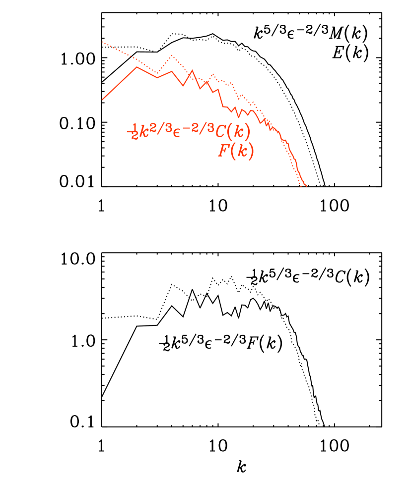
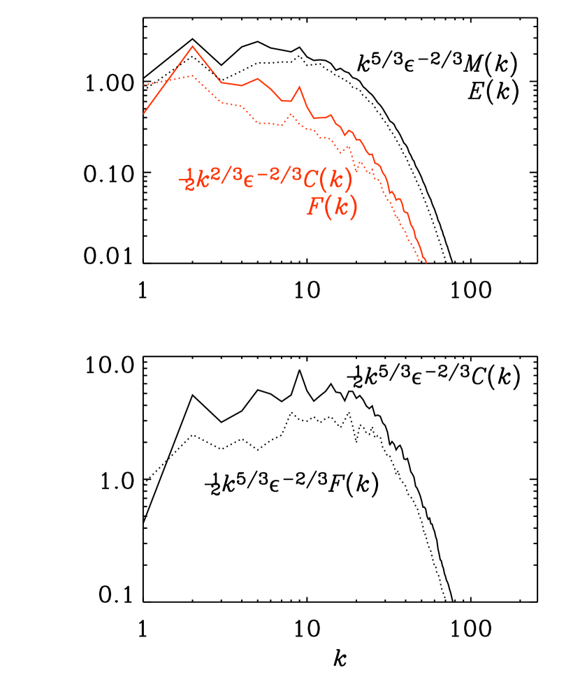
Since both $C(k)$ and $F(k)$ seem to scale like $k^{-5/3}$ in the inertial range, both helicities are governed by contributions from large scales. This implies in particular that the small scale current helicity, $\langle{\@vec{j}}\cdot{\@vec{b}}\rangle$, and hence also $\tilde{\alpha}_{\rm M}$, should not depend on the length of the inertial range and hence should be independent of $R_{\rm m}$. If this were not the case, i.e. if the magnetic field were fully helical with a $k^{-2/3}$ current helicity spectrum, $\tilde{\alpha}_{\rm K}$ would be asymptotically proportional to $R_{\rm m}^{1/4}$ (Blackman & Brandenburg 2002). Our results suggest that this is not the case here. This seems to be in conflict with earlier results for helical dynamos (Brandenburg 2001), but those results were at 4 times smaller resolution ($120^{3}$ instead of $512^{3}$ meshpoints) and the forcing was at 3 times smaller scale, so the effective length of the inertial range was 12 times smaller and hence completely absent. What remains true, however, is that the field is nearly fully helical at the energy carrying scale, i.e. at wavenumber $k_{\rm f}$.

7 Kinetically vs magnetically forced turbulence

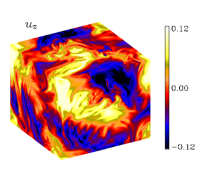
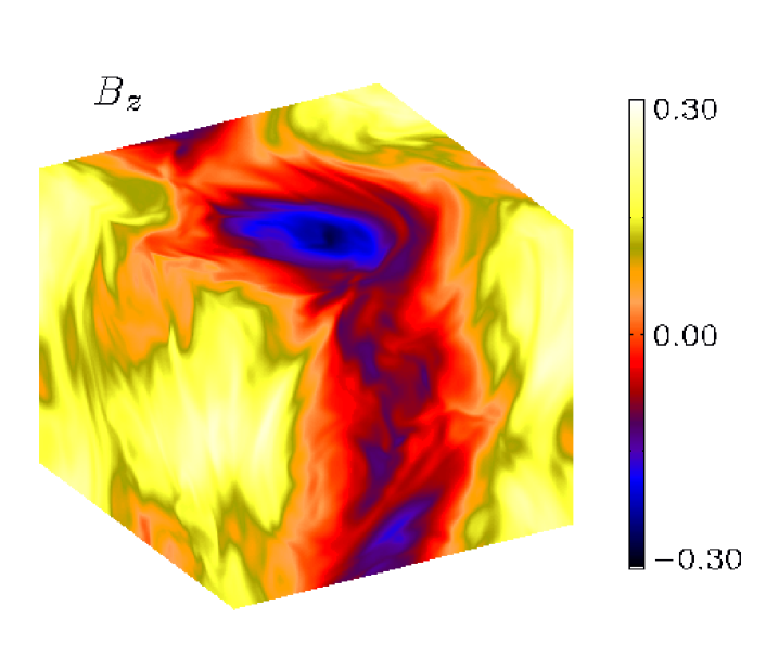
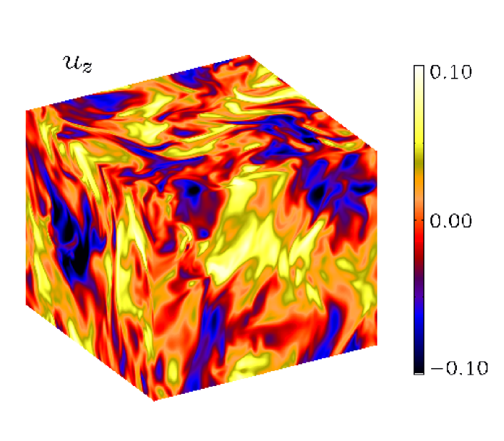
In order to gain more insight into the nature of the turbulence in kinetically and magnetically forced cases we show visualizations of the field-aligned components of velocity and magnetic field, $u_{z}$ and $B_{z}$, respectively. In the kinetically driven case we see a large scale pattern in velocity, consistent with power at the expected energy-carrying scale corresponding to the forcing wavenumber $k_{\rm f}=1.5$; see Fig. 10. The magnetic field, on the other hand, is dominated by smaller scale structures. The strength of the imposed field is still less than the equipartition value ($B_{0}/B_{\rm eq}\approx 0.4$) and there is no obvious anisotropy. Although the velocity field is helical, there is no obvious large-scale pattern in the magnetic field. There are two possible reasons for this: lack of scale separation (see Sect. V of Haugen et al. 2004) and suppression of large scale dynamo action by the large scale field (Montgomery et al. 2002, Brandenburg & Matthaeus 2004).

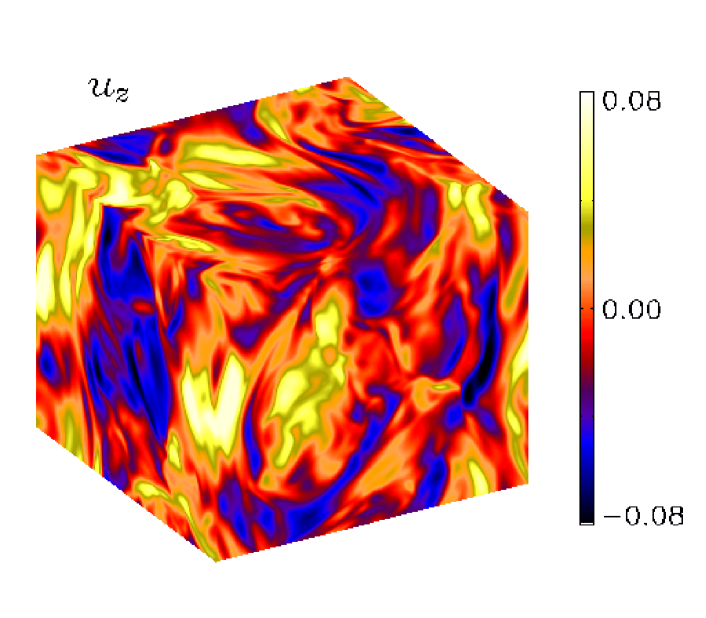
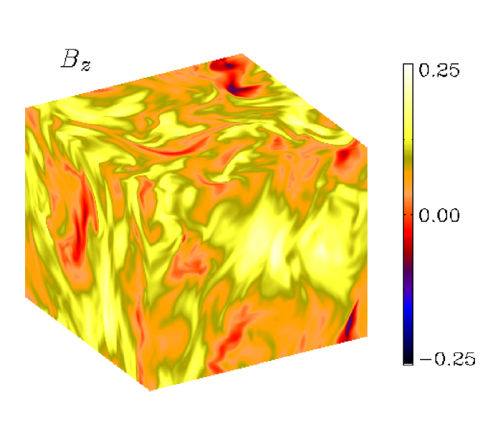
The magnetically driven case is quite different. There seems to be a large scale pattern in the magnetic field (Fig. 11). Although there is no scale separation, it is possible to drive a larger scale field in this case. The main difference is that in the kinetically driven case, dynamo-generated large scale and small scale fields have opposite sign of current helicity (Brandenburg 2001). In the absence of sufficient scale separation this leads to cancelation. In the magnetically driven case the current helicity has the same sign at all scales, so there is no cancellation and therefore the build-up of a large scale field is possible. However, when the field is too strong ($B_{0}=0.1$, corresponding to $B_{0}/B_{\rm eq}\approx 1$) no large scale pattern in the magnetic field develops; see Fig. 12.

8 Conclusions

Although a closure hypothesis of the form $\overline{\@vec{T}}=-\overline{\@vec{\cal E}}/\tau$ has a plausible physical interpretation as a relaxation term, (Blackman & Field 2002), it is nevertheless quite crude and lacks a rigorous physical basis. Nevertheless, on empirical grounds this closure assumption is quite appealing. First of all, unlike the first order smoothing approximation, MTA provides a natural and convincing explanation for the $\overline{{\@vec{j}}\cdot{\@vec{b}}}$ correction term to the $\alpha$ effect in Eq. (10). This is indeed a key ingredient to the dynamical quenching model (Kleeorin & Ruzmaikin 1982), where the evolution of $\overline{{\@vec{j}}\cdot{\@vec{b}}}$ is obtained by solving the magnetic helicity equation for the small scale field. The dynamical evolution of the $\overline{{\@vec{j}}\cdot{\@vec{b}}}$ term provides a good model for the resistively limited saturation (Field & Blackman 2002, Blackman & Brandenburg 2002, Subramanian 2002), which is seen in helically forced simulations in periodic boxes (Brandenburg 2001, Mininni et al. 2005). Another appealing property of MTA is that the additional time derivative, $\partial\overline{\@vec{\cal E}}/\partial t$ in Eq. (4), restores causality and prevents infinitely fast signal propagation. In the case of turbulent passive scalar diffusion, one can easily see that this term turns the heat equation into a damped wave equation, where the maximum signal speed is the rms velocity of the turbulence (Brandenburg et al. 2004).

One of the striking features of the dynamical quenching model is that the resistively limited saturation and the resistive quenching of the effective $\alpha$ can already be explained without invoking any explicit $R_{\rm m}$ dependence of $\tau$. Instead, the $R_{\rm m}$ dependence of the steady state values of $\alpha$ emerges solely as a result of magnetic helicity conservation and might hence be alleviated if there is a helicity flux that offsets magnetic helicity conservation (Blackman & Field 2000, Kleeorin et al. 2000, 2002, Vishniac & Cho 2001, Subramanian & Brandenburg 2004, Brandenburg & Sandin 2004, Brandenburg 2005, Brandenburg & Subramanian 2005b). However, there is no compulsory reason that there might not be an explicit $R_{\rm m}$ dependence of $\tau$ after all. Our present simulations begin to shed some light on this question. However, the results are still not as clear cut as one would like them to be. Looking at Fig. 6, it is evident that for $R_{\rm m}\leq 100$, St is independent of $R_{\rm m}$ and depends only on ${\@vec{B}}_{0}$; cf. the uniform decrease of St between the first and second panels of Fig. 6. However, for $R_{\rm m}>100$, St may actually decrease with $R_{\rm m}$, although the error bars also increase. If this decrease is indeed real, it might indicate that the closure hypothesis adopted here is too simplistic.

We should emphasize that, although we have in this work focused on the $\alpha$ effect, this is not the only effect that produces large scale dynamo action. An example is the shear–current effect of Rogachevskii & Kleeorin (2003, 2004). Here the electromotive force has a component in the direction of $-\overline{\@vec{W}}\times\overline{\@vec{J}}$, where $\overline{\@vec{W}}=\mbox{\boldmath$\nabla$}{}\times\overline{\@vec{U}}$ is the vorticity of the mean flow. (In the present work this effect is of course absent because there is no mean flow and our mean fields are defined as volume averages, so $\overline{\@vec{J}}=0$.) Our work is relevant even in this nonhelical case because, like the $\alpha$ effect, the $\overline{\@vec{W}}\times\overline{\@vec{J}}$ effect produces mean fields that are helical. Depending on the amount of magnetic helicity losses from open boundaries, there will be a tendency to limit the production of net magnetic helicity within the domain, so small scale current helicity of opposite sign must be produced at the same time as large scale field is generated. The presence of small scale current helicity implies that there must be a finite $\alpha_{\rm M}$. This is an example where there can be an $\alpha_{\rm M}$ term even though $\alpha_{\rm K}=0$. Related examples where $\alpha_{\rm K}=0$, but $\alpha_{\rm M}\neq 0$, are the reversed field pinch (e.g. Ho et al. 1989), and the so-called selective decay (e.g. Montgomery et al. 1978), as described in Blackman & Brandenburg (2002) and Yousef et al. (2003). Another example where $\alpha_{\rm K}=0$, but $\alpha_{\rm M}\neq 0$, is the Vishniac & Cho (2001) mechanism whereby dynamo action is accomplished through the current helicity flux that drives $\alpha_{\rm M}$; see Brandenburg & Subramanian (2005b) for model calculations showing that this effect produces saturation field strengths independent of the magnetic Reynolds number when the flux exceeds a certain threshold.

In the present paper we have only discussed the case where the helicity of the turbulence is driven explicitly. Although this is a common assumption that allows progress to be made in that the flow can be taken to be statistically isotropic, it should be noted that in astrophysical applications helicity is usually introduced by the interaction between stratification and rotation (Krause & Rädler 1980). To calculate this effect, MTA has to be used once more (e.g. Rädler et al. 2003), which then renders the $\alpha$ effect proportional to $\tau^{2}$. Nevertheless, as is emphasized in Brandenburg & Subramanian (2005a), also in this case the $\alpha$ effect is attenuated by the current helicity contribution from the small scale field.

Figure 10: Visualizations of $u_{z}$ (left) and $b_{z}$ (right) in the kinetically forced case. $B_{0}=0.03$, $\nu=\eta=2\times 10^{-4}$, $k_{\rm f}=1.5$, $512^{3}$ meshpoints.

Figure 11: Visualizations of $u_{z}$ (left) and $b_{z}$ (right) in the magnetically forced case. $B_{0}=0.03$, $\nu=\eta=2\times 10^{-4}$, $k_{\rm f}=1.5$, $512^{3}$ meshpoints.

Figure 12: Same as Fig. 11, but for $B_{0}=0.1$. There is no clear evidence for a large scale field.

Earlier simulations of helical dynamos (no imposed field) suggested that the field is bihelical, i.e. with one sign of helicity at large scales, corresponding to wavenumber $k_{1}$, and the opposite sign at small scales, corresponding to wavenumber $k_{\rm f}$ (Brandenburg 2001). If the field were to continue to be nearly fully helical even at smaller scales, this would have implied that $\tilde{\alpha}_{\rm M}$ would be attenuated by a $R_{\rm m}^{1/4}$ factor (Blackman & Brandenburg 2002). Our present results suggest that this is not the case. In agreement with both closure calculations (André & Lesieur 1977) and direct numerical simulations (Borue & Orszag 1997) we find approximate $k^{-5/3}$ scaling for the kinetic helicity (see also Ditlevsen & Giuliani 2001). Again, this implies that the velocity field is not fully helical beyond wavenumber $k_{\rm f}$, so $\tilde{\alpha}_{\rm K}$ should also be independent of $R_{\rm m}$. This is indeed the case, except for very small values of $R_{\rm m}$.

There are various ways of extending the present studies of turbulent transport to other fields. An obvious possibility is turbulent viscosity and the $\Lambda$ effect for modeling the Reynolds stress tensor (Käpylä et al. 2005). For example, one would expect the relaxation time to depend on the angular velocity (Kitchatinov & Rüdiger 1993). This dependence could be measured in a similar way as the dependence on the magnetic field studied in the present paper. Another related application is the study of passive scalar transport in the present of rotation. Both aspects are quite essential for many astrophysical applications.

Appendix A The forcing function

For completeness we specify here the forcing function used in the present paper. It is defined as

$$\mbox{\boldmath$f$}{}(\mbox{\boldmath$x$}{},t)={\rm Re}\{N\mbox{\boldmath$f$}{}_{\mbox{\boldmath$k$}{}(t)}\exp[{\rm i}\mbox{\boldmath$k$}{}(t)\cdot\mbox{\boldmath$x$}{}+{\rm i}\phi(t)]\},$$ (22)

where $x$ is the position vector. The wavevector $\mbox{\boldmath$k$}{}(t)$ and the random phase $-\pi<\phi(t)\leq\pi$ change at every time step, so $\mbox{\boldmath$f$}{}(\mbox{\boldmath$x$}{},t)$ is $\delta$-correlated in time. For the time-integrated forcing function to be independent of the length of the time step $\delta t$, the normalization factor $N$ has to be proportional to $\delta t^{-1/2}$. On dimensional grounds it is chosen to be $N=f_{0}c_{\rm s}(|\mbox{\boldmath$k$}{}|c_{\rm s}/\delta t)^{1/2}$, where $f_{0}$ is a nondimensional forcing amplitude. The value of the coefficient $f_{0}$ is chosen such that the maximum Mach number stays below about 0.5; in practice this means $f_{0}=0.01\ldots 0.05$, depending on the average forcing wavenumber. At each timestep we select randomly one of many possible wavevectors in a certain range around a given forcing wavenumber. The average wavenumber is referred to as $k_{\rm f}$. Two different wavenumber intervals are considered: $1...2$ for $k_{\rm f}=1.5$ and $4.5...5.5$ for $k_{\rm f}=5$. We force the system with transverse helical waves,

$$\mbox{\boldmath$f$}{}_{\mbox{\boldmath$k$}{}}=\mbox{\boldmath${\sf R}$}{}\cdot\mbox{\boldmath$f$}{}_{\mbox{\boldmath$k$}{}}^{\rm(nohel)}\quad\mbox{with}\quad{\sf R}_{ij}={\delta_{ij}-{\rm i}\sigma\epsilon_{ijk}\hat{k}_{k}\over\sqrt{1+\sigma^{2}}},$$ (23)

where $\sigma=1$ for positive helicity of the forcing function,

$$\mbox{\boldmath$f$}{}_{\mbox{\boldmath$k$}{}}^{\rm(nohel)}=\left(\mbox{\boldmath$k$}{}\times\hat{\mbox{\boldmath$e$}}{}\right)/\sqrt{\mbox{\boldmath$k$}{}^{2}-(\mbox{\boldmath$k$}{}\cdot\hat{\mbox{\boldmath$e$}}{})^{2}},$$ (24)

is a non-helical forcing function, and $\hat{\mbox{\boldmath$e$}}{}$ is an arbitrary unit vector not aligned with $k$; note that $|\mbox{\boldmath$f$}{}_{\mbox{\boldmath$k$}{}}|^{2}=1$.

Appendix B Modified Keinigs relation

The $R_{\rm m}$ dependence of $\alpha$ can generally be understood as a direct consequence of magnetic helicity conservation (Gruzinov & Diamond 1994). Dotting Eq. (6) with the vector potential ${\@vec{a}}$, where ${\@vec{b}}=\mbox{\boldmath$\nabla$}{}\times{\@vec{a}}$, and adding the corresponding evolution of $\dot{{\@vec{a}}}\cdot{\@vec{b}}$, averaging over a periodic volume, and using $({\@vec{u}}\times{\@vec{B}}_{0})\times{\@vec{b}}=-({\@vec{u}}\times{\@vec{b}})\cdot{\@vec{B}}_{0}$ we obtain

$${\textstyle{1\over 2}}{{\rm d}{}\over{\rm d}{}t}\langle{\@vec{a}}\cdot{\@vec{b}}\rangle=-\langle{\@vec{u}}\times{\@vec{b}}\rangle\cdot{\@vec{B}}_{0}-\eta\langle{\@vec{j}}\cdot{\@vec{b}}\rangle+\langle{\@vec{b}}\cdot\mbox{\boldmath$f$}{}_{\rm mag}\rangle.$$ (25)

Using $\langle{\@vec{u}}\times{\@vec{b}}\rangle=\alpha{\@vec{B}}_{0}$, we find in the steady state

$$\alpha=-\eta{\langle{\@vec{j}}\cdot{\@vec{b}}\rangle\over{\@vec{B}}_{0}^{2}}+{\langle{\@vec{b}}\cdot\mbox{\boldmath$f$}{}_{\rm mag}\rangle\over{\@vec{B}}_{0}^{2}}.$$ (26)

The first term, which was already obtained in an early paper by Keinigs (1983), is manifestly $\eta$-dependent [see also Brandenburg & Matthaeus (2004) for a derivation of this term], but the second term is not. This explains the behavior seen in Fig. 2.

References

- (1) André, J.-C. & Lesieur, M. 1977, JFM, 81, 187
- (2) Blackman, E. G., & Field, G. F. 2000, MNRAS, 318, 724
- (3) Blackman, E. G., & Field, G. B. 2002, PRL, 89, 265007
- (4) Blackman, E. G., & Field, G. B. 2003, PhFl, 15, L73
- (5) Blackman, E. G., & Brandenburg, A. 2002, ApJ, 579, 359
- (6) Borue, V., & Orszag, S. A. 1997, PRE, 55, 7005
- (7) Brandenburg, A. 2001, ApJ, 550, 824
- (8) Brandenburg, A. 2005, ApJ, 625, 539
- (9) Brandenburg, A., & Matthaeus, W. H. 2004, PRE, 69, 056407
- (10) Brandenburg, A., & Sandin, C. 2004, A&A, 427, 13
- (11) Brandenburg, A., & Subramanian, K. 2005a, PhR, astro-ph/0405052 (in press)
- (12) Brandenburg, A., & Subramanian, K. 2005b, AN, 326, 400
- (13) Brandenburg, A., Käpylä, P., & Mohammed, A. 2004, PhFl, 16, 1020
- (14) Cattaneo, F., & Hughes, D. W. 1996, PRE, 54, R4532
- (15) Ditlevsen, P. D., & Giuliani, P. 2001, PRE, 63, 036304
- (16) Field, G. B., & Blackman, E. G. 2002, ApJ, 572, 685
- (17) Gruzinov, A. V., & Diamond, P. H. 1994, PRL, 72, 1651
- (18) Haugen, N. E. L., Brandenburg, A., & Dobler, W. 2004, PRE, 70, 016308
- (19) Ho, Y. L., Prager, S. C., Schnack, D. D. 1989, PRL, 62, 1504
- (20) Käpyla, P. J., Korpi, M. J., Ossendrijver, M., & Tuominen, I. 2005, AN, 326, 186
- (21) Keinigs, R. K. 1983, PhFl, 26, 2558
- (22) Kitchatinov, & L. L., Rüdiger, G. 1993, A&A, 276, 96
- (23) Kitchatinov, L. L., Rüdiger, G., & Pipin, V. V. 1994, AN, 315, 157
- (24) Kleeorin, N. I., & Ruzmaikin, A. A. 1982, Magnetohydrodynamics, 18, 116
- (25) Kleeorin, N. I., Rogachevskii, I. V., Ruzmaikin, A. A. 1990, Sov. Phys. JETP, 70, 878
- (26) Kleeorin, N. I., Mond, M., & Rogachevskii, I. 1996, A&A, 307, 293
- (27) Kleeorin, N. I, Moss, D., Rogachevskii, I., & Sokoloff, D. 2000, A&A, 361, L5
- (28) Kleeorin, N. I, Moss, D., Rogachevskii, I., & Sokoloff, D. 2002, A&A, 387, 453
- (29) Krause, F., & Rädler, K.-H. 1980, Mean-Field Magnetohydrodynamics and Dynamo Theory (Pergamon Press, Oxford)
- (30) Mininni, P. D., Gómez, D. O., Mahajan, S. M. 2005, ApJ, 619, 1019
- (31) Moffatt, H. K. 1972, JFM, 53, 385
- (32) Moffatt, H. K. 1978, Magnetic Field Generation in Electrically Conducting Fluids (Cambridge University Press, Cambridge)
- (33) Montgomery, D., Turner, L., & Vahala, G. 1978, PhFl, 21, 757
- (34) Montgomery, D., Matthaeus, W. H., Milano, L. J., & Dmitruk, P. 2002, Phys. Plasmas, 9, 1221
- (35) Pouquet, A., Frisch, U., & Léorat, J. 1976, JFM, 77, 321
- (36) Rädler, K.-H., Kleeorin, N., & Rogachevskii, I. 2003, GApFD, 97, 249
- (37) Rogachevskii, I., & Kleeorin, N. 2003, PRE, 68, 036301
- (38) Rogachevskii, I., & Kleeorin, N. 2004, PRE, 70, 046310
- (39) Rüdiger, G. 1974, AN, 295, 275
- (40) Rüdiger, G. 1989, Differential rotation and stellar convection: Sun and solar-type stars (Gordon & Breach, New York)
- (41) Rüdiger, G. & Kitchatinov, L. L. 1993, A&A, 269, 581
- (42) Subramanian, K. 2002, Bull. Astr. Soc. India, 30, 715
- (43) Subramanian, K., & Brandenburg, A. 2004, PRL, 93, 205001
- (44) Vainshtein, S. I. & Kitchatinov, L. L. 1983, GApFD, 24, 273
- (45) Vishniac, E. T., & Cho, J. 2001, ApJ, 550, 752
- (46) Yousef, T. A., Brandenburg, A., & Rüdiger, G. 2003, A&A, 411, 321