Photoevaporation Flows in Blister $\mathrm{H\,\scriptstyle II}$ Regions:
I. Smooth Ionization Fronts and Application to the Orion Nebula

Abstract

We present hydrodynamical simulations of the photoevaporation of a cloud with large-scale density gradients, giving rise to an ionized, photoevaporation flow. The flow is found to be approximately steady during the large part of its evolution, during which it can resemble a “champagne flow” or a “globule flow” depending on the curvature of the ionization front. The distance from source to ionization front and the front curvature uniquely determine the structure of the flow, with the curvature depending on the steepness of the lateral density gradient in the neutral cloud.

We compare these simulations with both new and existing observations of the Orion nebula and find that a model with a mildly convex ionization front can reproduce the profiles of emission measure, electron density, and mean line velocity for a variety of emitting ions on scales of $10^{17}$–$10^{18}\,\mathrm{cm}$. The principal failure of our model is that we cannot explain the large observed widths of the [$\mathrm{O\,\scriptstyle I}$] 6300 Å line that forms at the ionization front.

1. Introduction

$\mathrm{H\,\scriptstyle II}$ regions, formed by the action of ionizing photons from a high-mass star on the surrounding gas, often occur in highly inhomogeneous environments. Most $\mathrm{H\,\scriptstyle II}$ regions are found close to high density concentrations of molecular gas and, for those regions that are optically visible, there is a tendency for the ionized emission to be blueshifted with respect to the molecular emission (Israel, 1978). Since optically visible $\mathrm{H\,\scriptstyle II}$ regions must be on the near side of the molecular gas, this implies that the ionized gas is flowing away from the molecular cloud. The archetypal and best-studied example of such a “blister-type” $\mathrm{H\,\scriptstyle II}$ region is the nearby Orion nebula, which is ionized by the O7 V star, $\theta^{1}$ Ori C (for recent reviews, see O’Dell, 2001a; Ferland, 2001; O’Dell, 2001b). This compact $\mathrm{H\,\scriptstyle II}$ region, which lies in front of the molecular cloud OMC 1, shows a bright core of ionized emission, approximately $10^{18}\,\mathrm{cm}$ in diameter, surrounded by a fainter halo that extends out to distances of order $10^{19}\,\mathrm{cm}$ (Subrahmanyan et al., 2001). Surprisingly, the thickness along the line of sight of the layer responsible for the bulk of the ionized emission in the core of the nebula is only $\sim 2\times 10^{17}\,\mathrm{cm}$ (e.g., Baldwin et al., 1991; Wen & O’Dell, 1995), which is significantly smaller than both the lateral extent of the core and the deduced distance between the ionizing star and the front, which is also of order $10^{18}\,\mathrm{cm}$. Three-dimensional reconstruction of the shape of the nebula’s principal ionization front (Wen & O’Dell, 1995) shows the front to have a saddle-shaped structure, with a slight concavity in the NS direction and a slight convexity in the EW direction (see O’Dell, 2001b, Figure 3). In both cases the radius of curvature is large compared with star-front distance, although there are also many smaller scale irregularities in the front, with the most prominent of these being associated with the “Bright Bar” in the SE region of the nebula. Extensive spectroscopic studies of the Orion nebula have been carried out to determine the velocity structure in the ionized gas (Kaler, 1967; Balick et al., 1974; Pankonin et al., 1979; O’Dell et al., 1993; Henney & O’Dell, 1999; O’Dell et al., 2001; Doi et al., 2004). Although these show a wealth of fine-scale structure, the fundamental result is that lines from the more highly ionized species such as H$\alpha$ and [$\mathrm{O\,\scriptstyle III}$] are blue-shifted by approximately $10\,\mathrm{km\,s^{-1}}$ with respect to the molecular gas of OMC-1, which lies behind the nebula. Lines from intermediate-ionization species such as [$\mathrm{S\,\scriptstyle II}$] and [$\mathrm{N\,\scriptstyle II}$] being found at intermediate velocities. All these considerations lead to a basic model of the nebula as a thin layer of ionized gas that is streaming away from the molecular cloud, as was first proposed by Zuckerman (1973).

Despite, or perhaps because of, the mass of observational data that has been accumulated on the Orion nebula, no attempt has been made to develop a self-consistent dynamical model of the ionized flow since the early work of Vandervoort (1963, 1964). Most modern models of the nebula have concentrated great effort on details of the atomic physics and radiative transfer (Baldwin et al., 1991; Rubin et al., 1991) and, while these have been quite successful in explaining the ionization structure of the nebula, they implicitly assume a static configuration and are forced to adopt ad hoc density configurations that have no physical basis. The importance of photoevaporation flows has been recognized in the context of the modeling of other $\mathrm{H\,\scriptstyle II}$ regions Hester et al. (1996); Scowen et al. (1998); Sankrit & Hester (2000); Moore et al. (2002) but again no attempt has been made to treat the dynamics in a consistent manner. More recently, steady-state dynamic models of weak-D ionization fronts have been developed and applied to the Orion nebula (Henney et al., 2005), with some success in explaining the structure of the Bright Bar, where the ionization front is believed to be viewed edge-on. However, the one-dimensional, plane-parallel nature of these models renders them incapable of capturing the global geometry of the nebula and indeed they completely fail to reproduce the observed correlation between line velocity and ionization potential.

The evolution of an $\mathrm{H\,\scriptstyle II}$ region in an inhomogeneous medium was first studied by Tenorio-Tagle (1979), who considered the “break-out” of a photoionized region from the edge of a dense cloud, such as would occur if a high-mass star formed inside, but close to the edge of, a molecular cloud. Once the ionization front reaches the edge of the cloud, it rapidly propagates through the low-density intercloud medium, followed by a strong shock driven by the higher pressure ionized cloud material. At the same time, a rarefaction wave propagates back into the ionized cloud, giving rise to a “champagne flow” in which the $\mathrm{H\,\scriptstyle II}$ region is ionization-bounded on the high density side and density-bounded on the low-density side and the ionized gas flows down the density gradient. This work has been extended in many subsequent papers using both one-dimensional and two-dimensional numerical simulations (Bodenheimer et al., 1979; Bedijn & Tenorio-Tagle, 1981; Yorke et al., 1982; Franco et al., 1989; Comeron, 1997), which generally concentrate on non-steady aspects of the flow.

Another scenario that has been extensively studied is the ionization of a neutral globule by an external radiation field (Pottasch, 1956; Dyson, 1968; Tenorio-Tagle & Bedijn, 1981; Bedijn & Tenorio-Tagle, 1984; Bertoldi, 1989; Bertoldi & McKee, 1990), to form what is variously referred to as an ionized photoevaporation or photoablation flow. In this case, after an initial transient phase in which the globule is compressed, the ionization front propagates very slowly into the globule and the ionized flow is steady to a good approximation. Although originally developed in the context of bright rims and globules in $\mathrm{H\,\scriptstyle II}$ regions, similar models have more recently been applied to the photoevaporation of circumstellar accretion disks (Johnstone et al., 1998; Henney & Arthur, 1998) and cometary knots in planetary nebulae (López-Martín et al., 2001; O’Dell et al., 2000). In all these cases, the ionization front has positive (convex) curvature, and the ionized gas accelerates away from the ionization front in a transonic, spherically divergent flow.

In a strictly plane-parallel geometry, a time-stationary champagne flow cannot exist. This is because, in the absence of body forces, the acceleration of a steady plane-parallel flow is proportional to the gradient of the sound speed, which is roughly constant in the photoionized gas. However, it has recently been shown (Henney, 2003) that a steady, ionized, isothermal, transonic, divergent flow can exist even if the ionization front is flat, so long as the ionizing source is at a finite distance from the front. In such a case, the divergence of the radiation field breaks the plane-parallel geometry and induces a (weaker) divergence in the ionized flow, allowing it to accelerate (an expanded and corrected version of this derivation is presented in Appendix A below). It is natural to speculate that a steady flow may also be possible even if the front has negative (concave) curvature, so long as the radius of curvature of the front is greater than its distance from the ionizing source. By this means, the champagne flow problem can be effectively reduced to a modified version of the globule flow problem.

In order to investigate this possibility, we here present hydrodynamical simulations of the photoionization of a neutral cloud with large-scale density gradients and develop a taxonomy of the resulting $\mathrm{H\,\scriptstyle II}$ region flow structure and dynamics. We concentrate on the quasi-stationary stage of the $\mathrm{H\,\scriptstyle II}$ region evolution, in which the structure changes slowly compared with the dynamical timescale of the ionized flow, with the result that the flow is approximately steady in the frame of the front. Depending on the curvature of the ionization front, our models can resemble both “blister flows” (Israel, 1978) if the curvature is negative (concave), or “bright rims” (Pottasch, 1956), if the curvature is positive (convex). The algorithm, initial conditions, and parameters of these numerical simulations are described in § 2 and their results are set out in § 3. In § 4 we derive empirical parameters for the Orion nebula that will allow us to make meaningful comparisons with our models. These comparisons are carried out in § 5. In § 6 we discuss the implications of our model comparisons to Orion and outline some shortcomings of the present simulations that will be addressed in future work. In § 7 we draw the conclusions of our paper. Finally, we present some more technical material in two appendices. The first derives an approximate analytic model for the flow from a plane ionization front, while the second investigates the question of whether the ionization fronts in our simulations are D-critical.

2. Numerical Simulations

In this section we present time-dependent numerical hydrodynamic simulations of the photoionization of neutral gas by a point source offset from a plane density interface.

2.1. Implementation Details

The Euler equations are solved in two-dimensional cylindrical geometry, using a second-order, finite-volume, hybrid scheme, in which alternate timesteps are calculated by the Godunov method and the Van Leer flux-vector splitting method (Godunov, 1959; van Leer, 1982). The radiative transfer of the ionizing radiation is carried out by the method of short characteristics (Raga et al., 1999), with the only source of ionizing opacity being photoelectric absorption by neutral hydrogen. Only one frequency of radiation is included but radiation-hardening is accounted for by varying the effective photoabsorption cross-section as a function of optical depth (Henney et al., 2005). The diffuse field is treated by the on-the-spot approximation. Dust opacity is not explicitly included in our calculations but is treated to zeroth order by merely reducing the stellar ionizing luminosity to account for absorption by grains. As shown in Appendix A, this is a rather good approximation at least in the case of a flow from a plane ionization front.

Ionization and recombination of hydrogen is calculated by exact integration of the relevant equations over a numerical timestep. Heating and cooling of the gas are calculated by a second-order explicit scheme. The only heating process considered is the photoionization of hydrogen, with the energy deposited per ionization increasing with optical depth according to the hardening of the radiation field. The most important cooling processes included are collisional excitation of Lyman alpha, collisional excitation of neutral and ionized metal lines (assuming standard ISM abundances), and hydrogen recombination. Other cooling processes included in the code, such as collisional ionization and bremsstrahlung, are only important at higher temperatures than are found in the current simulations.

2.2. Initial Conditions

At the beginning of the simulation, the ionizing source is placed at $r=0$, $z=z_{0}$, and the computational domain is filled with neutral gas with a separable density distribution:

$$\rho(r,z)=\rho_{0}F(r)G(z).$$ (1)

For comparison with the analytic model of Appendix A, we wish to contrive a neutral density distribution that will ensure that the ionization front stays approximately flat throughout its evolution, although we will also investigate the flow from curved fronts.

The initial flatness of the ionization front is guaranteed by choosing $G(z)$ to be a step function between a very low value (that will be ionized in a recombination time) and a very high value (that will trap the ionization front at the interface). In practice, we choose the function

$$\log_{10}G(z)=\delta\tanh((z-z_{1})/h_{1}),$$ (2)

where $h_{1}$ is the thickness of the interface, which occurs at a height $z_{1}$ ($>z_{0}$). The density contrast between the two sides is $10^{2\delta}$.

In order for the ionization front to remain flat as it propagates into the dense neutral gas above the interface, we let the initial density fall off gradually in the radial direction according to the function

$$F(r)=\left[1+\left(\frac{r}{z_{1}-z_{0}}\right)^{2}\right]^{-\alpha},$$ (3)

where $\alpha$ is an adjustable parameter controlling the steepness of the distribution. The analytic model of Appendix A suggests that $\alpha=1$ should ensure that all parts of the ionization front propagate at the same speed. Choosing smaller values of $\alpha$ should mean that the front propagates fastest along the symmetry axis and so the front becomes concave with time. Conversely, larger values of $\alpha$ will cause the front to propagate faster away from the axis and so become convex with time.

A characteristic temperature, $T_{0}$, is chosen, which corresponds to gas at a density of $\rho_{0}$. The temperature distribution throughout the grid is then set so as to give a constant pressure where $\rho>\rho_{0}$ and a constant temperature where $\rho<\rho_{0}$.

In this paper we follow Shu (1992) in denoting gas velocities in the frame of reference of the ionizing star by $u$, gas velocities in the frame of reference of the ionization front by $v$, and pattern speeds of ionization, heating, and shock fronts by $U$.

2.3. Model Parameters

We present three different models, which illustrate the effect of different radial density distributions in the neutral gas, with $\alpha=0$ (Model A), $\alpha=1$ (Model B), and $\alpha=2$ (Model C). All other parameters are identical between the three models and are chosen to be representative of a compact $\mathrm{H\,\scriptstyle II}$ region such as the Orion nebula. The simulation is carried out on a $512\times 512$ grid, with sides of length $1\,\mathrm{pc}$. The source has an ionizing luminosity $Q_{\mathrm{H}}=10^{49}\,\mathrm{s^{-1}}$, with a $40,000\,\mathrm{K}$ black-body spectrum, and is placed half-way up the simulation grid on the $z$-axis. The characteristic density for the simulation is set at $\rho_{0}=10^{4}m\,\mathrm{cm^{-3}}$, where $m$ is the mean mass per nucleon (assumed to be $1.3m_{\mathrm{H}}$). The separation, $z_{1}-z_{0}$, between the source and the density interface is chosen so that the analytic steady-state model of Appendix A below would give a peak ionized density of $\rho_{0}/m=10^{4}\,\mathrm{cm^{-3}}$ in the photoevaporation flow. This yields $z_{1}-z_{0}=4.8\times 10^{17}\,\mathrm{cm}=0.155\,\mathrm{pc}$. The initial density contrast across the interface is set at $\delta=2$, yielding $n=10^{6}\,\mathrm{cm^{-3}}$ on the high-density side and $n=10^{2}\,\mathrm{cm^{-3}}$ on the low-density side. The thickness of the interface is set at $h_{1}=0.3(z_{1}-z_{0})$ and the characteristic temperature is set at $T_{0}=600\,\mathrm{K}$.

In order to make the simulations feasible, it is necessary to use a hydrogen photoionization cross-section that is considerably smaller than the physically correct value, which would be roughly $\sigma_{0}=3\times 10^{-18}\,\mathrm{cm}^{2}$ for unhardened radiation from a $40,000\,\mathrm{K}$ black body (Henney et al., 2005, Appendix A). In these models, we instead use a value of $\sigma_{0}=5\times 10^{-20}\,\mathrm{cm}^{2}$, which is 60 times smaller. This is necessary in order to properly resolve the deep part of the ionization front (at $\tau\simeq 10$) where the initial heating of the photoevaporation flow occurs. Failure to resolve this region results in spurious large-magnitude oscillations in the flow. Using a smaller value of $\sigma_{0}$ increases the width of the ionization front but has a negligible effect on the kinematic behavior of the gas once it is fully ionized. We have studied the effect of increasing or decreasing $\sigma_{0}$ and find that our results are generally not affected, with the exception of some specific points noted below.

Although each model is calculated for specific values of the length scale and ionizing luminosity, they may be safely rescaled to different values so long as the ionization parameter remains the same, which will guarantee that the ionization fractions in the model are not affected by the rescaling. This is because the dimensionless form of the gas-dynamical, radiation transfer and ionization equations contain only a handful of dimensionless parameters (for example Henney et al., 2005, Appendix A). The only one of these that depends on the density and length scales is a dimensionless form of the ionization parameter: $\tau_{*}=n_{0}\sigma_{0}\ell_{0}$, where $\ell_{0}$ is the length scale.

One can then use the Strömgren relation, $Q_{\mathrm{H}}\propto n_{0}^{2}\ell_{0}^{3}$, to eliminate the density and find that a fixed ionization parameter requires a fixed ratio of $Q_{\mathrm{H}}/\ell_{0}$. All times should also be scaled proportionately to $\ell$. Furthermore, it is even possible to scale $Q_{\mathrm{H}}$ and $\ell$ independently, subject to the understanding that one is also thereby scaling the effective photoionization cross-section as $\sigma_{0}\propto(\ell/Q_{\mathrm{H}})^{1/2}$.

3. Model Results

3.1. Early Evolution of the Models

Figure 1.— (a) Evolution with time of the axial distance from the star to the shock front, $z_{\mathrm{s}}$ (upper line), heating front $z_{\mathrm{h}}$ (middle line), and ionized density peak, $z_{\mathrm{p}}$ (lower line), all for Model B. (b) Evolution of $z_{\mathrm{p}}$ for the different models: A (solid line), B (dashed line), and C (dotted line). (c) Same as b but for the evolution of $z_{\mathrm{h}}$. (d) Same as b but for the evolution of $z_{\mathrm{s}}$.

The initial evolution of all three models is the same: the low-density gas below the interface is completely ionized on a recombination timescale of $\sim 1000\,\mathrm{yr}$. At the interface itself, the ionization/heating front at first penetrates to gas of density $\sim\rho_{0}$, which is heated to $\simeq 9000\,\mathrm{K}$, and achieves a thermal pressure 30 times higher than the pressure in the cold neutral gas. This drives a shockwave up the density ramp at a speed $u_{\mathrm{s}}\simeq(\rho_{\mathrm{i}}/\rho_{\mathrm{n}})^{1/2}c_{\mathrm{i}}$, where $\rho_{\mathrm{i}}$ is the ionized density, $c_{\mathrm{i}}$ is the ionized sound speed, and $\rho_{\mathrm{n}}$ is the pre-shock neutral density. The shock can be first discerned in the simulations after about $3000\,\mathrm{yr}$, at which time its speed is $u_{\mathrm{s}}\simeq 5\,\mathrm{km\,s^{-1}}$, falling to $\simeq 1\,\mathrm{km\,s^{-1}}$ by the time it reaches the top of the density ramp (after about $40,000\,\mathrm{yr}$). The time-evolution of the shock front position in the three models is almost identical during this early stage, as can be seen in Figure 1d.

At the same time as the shock propagates into the neutral gas, the warm gas expands down the density ramp, towards (and beyond) the star. Within $30,000\,\mathrm{yr}$ all the gas that was originally below the density interface has been swept off the grid by this flow, which accelerates up to about $20\,\mathrm{km\,s^{-1}}$. Initially, the ionized gas flows parallel to the $z$-axis but as time goes on the streamlines begin to diverge and the flow settles into a quasi-steady configuration, during which the properties of the ionized flow and the subsequent evolution of the ionization front vary significantly between the models.

In addition to the position of the shock front, $z_{\mathrm{s}}$, we make reference below to the position of the heating front, $z_{\mathrm{h}}$, which is a very thin layer at the very base of the evaporation flow, and also to the position of the ionized density peak, $z_{\mathrm{p}}$, formed by the opposing gradients in total density and ionization fraction. The time evolution of these three quantities is shown in Figure 1.

3.2. Properties of the Quasi-steady Flow

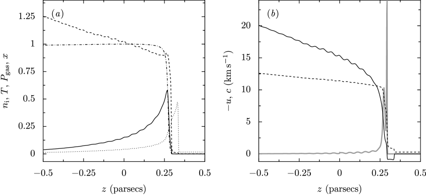
Figure 2.— Axial profiles of physical variables in Model B at an age of $78,000\,\mathrm{yr}$. (a) Ionized hydrogen density $n_{\mathrm{i}}$ (solid line, units of $10^{4}\,\mathrm{cm^{-3}}$), gas temperature $T$ (dashed line, units of $10^{4}\,\mathrm{K}$), pressure $P_{\mathrm{gas}}$ (dotted line, units of $10^{-7}\,\mathrm{dyne\,cm^{-2}}$), and ionization fraction (dot-dashed line). (b) Negative of the gas velocity in the reference frame of the star, $u$ (solid line), and isothermal sound speed (dashed line, both in $\mathrm{km\,s^{-1}}$), plus net heating rate (thick gray line, arbitrary units).

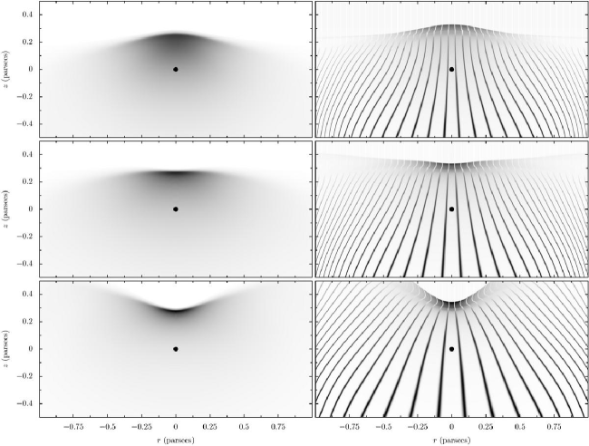
Figure 3.— Snapshot images of the three models (top to bottom: A, B, C) at a time of $78,000\,\mathrm{yr}$. Left column shows ionized hydrogen density as a linear negative grayscale, where black represents a density of $6600\,\mathrm{cm^{-3}}$. Right column shows gas pressure ($\mathrm{black}=6.1\times 10^{-8}\,\mathrm{dyne\,cm^{-2}}$) with superimposed streamlines whose darkness indicates magnitude of the gas velocity ($\mathrm{black}=20.1\,\mathrm{km\,s^{-1}}$). All grayscales are common between the models. The position of the ionizing star is indicated by a filled circle in each panel.

After the initial transient phase, the flow settles down into a long quasi-steady phase in which the flow properties change only on timescales much longer than the dynamic time for flow away from the ionization front. As we will show below, the flow structure, once normalized to the distance of the star from the front, seems to depend only on the curvature of the ionization front. During this quasi-steady phase the shock in the neutral gas is propagating at about $1\ \mathrm{km\,s^{-1}}$, as discussed in the previous section, and the post-shock gas moves at about three-quarters of this speed since it does does not cool strongly in our simulations. At the same time, the relative velocity between the ionization/heating front and the neutral gas immediately outside it is very low (for a D-critical front this would be $c_{\mathrm{n}}/2c_{\mathrm{i}}^{2}\simeq 0.05\ \mathrm{km\,s^{-1}}$, see Appendix B), so that the ionization front speed is also about three-quarters of the shock speed, leading to a steady thickening of the shocked neutral layer. However, this behavior is dependent on the cooling behavior of the shocked neutral gas, which we do not treat very realistically. Stronger cooling would cause the ionization and shock fronts to propagate at the same speed.

Details of the variation along the $z$ axis of various physical quantities for Model B are shown in Figure 2. Images of the distributions of ionized density and pressure in the models at a representative point in their evolution are shown in Figure 3, together with the flow streamlines.

3.2.1 Structure along the $z$-axis

The shock driven into the neutral gas is traced by the pressure (dotted line in Fig. 2a, grayscale in right-hand panels of Fig. 3), which peaks immediately behind the shock. The ionization front is traced by the ionization fraction (dot-dashed line in Fig. 2a) and the ionized density (solid line in Fig. 2a) shows a peak just inside the front. One can also see a heating front, best seen in the temperature (dashed line in Fig. 2a), which lies just outside the ionization front. The temperature shows a slight peak at the ionization front due to the radiation hardening.

The solid line in Figure 2 shows the negative of the gas velocity (i.e. velocity back towards the ionizing star). The neutral gas is initially accelerated away from the star by the shock, which gives the neutral shell a speed of $\sim+1\,\mathrm{km\,s^{-1}}$. In the ionization front it is accelerated back towards the star, quickly reaching speeds of $\sim-10\,\mathrm{km\,s^{-1}}$ and then continuing a gradual acceleration to $\sim-20\,\mathrm{km\,s^{-1}}$ before leaving the grid. The isothermal sound speed is shown by the dashed line in Figure 2b and it can be seen that the flow becomes supersonic shortly after passing the peak in the ionized density. The question of whether the fronts are D-critical is addressed in Appendix B. The net rate of energy deposition into the gas (photoionization heating minus collisional line cooling) is shown by the thick gray line in Figure 2b and always shows two peaks. These can be seen in more detail in Figure 4, which shows a log-log plot of various quantities as a function of the optical depth to ionizing radiation, $\tau=\int\langle\sigma\rangle n(\mathrm{H_{0}})\,dz$. The deeper of the two energy deposition peaks is the heating front, which occurs at an ionizing optical depth of $\tau\simeq 8$, where the ionization fraction is around $x\simeq 0.01$ and the gas density around $n\simeq 10^{5}\,\mathrm{cm^{-3}}$. In this front the gas is rapidly heated up to just under $10^{4}\,\mathrm{K}$ and accelerated up to $2$–$3\,\mathrm{km\,s^{-1}}$ but remains largely neutral (note that in Fig. 4 the velocity is now shown in the rest frame of the heating front, $v$). The second, broader peak, at $\tau=2$–$4$, coincides with the ionization of the gas at a roughly constant temperature and its gradual acceleration up to the ionized sound speed.

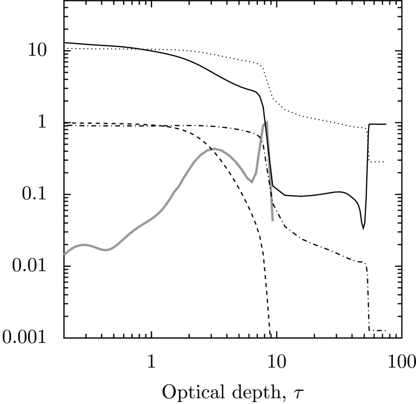
Figure 4.— Structure of the ionization front in Model B at an age of $78,000\,\mathrm{yr}$. Gas velocity with respect to the heating front, $v$, in $\mathrm{km\,s^{-1}}{}$ (solid line); ionization fraction, $x$ (dashed line); isothermal sound speed, $c$, in $\mathrm{km\,s^{-1}}{}$ (dotted line); temperature, $T/10^{4}\,\mathrm{K}$ (dot-dashed line); net energy deposition rate in arbitrary units (thick gray line).

3.2.2 Differences between the models

Despite the general similarities, there are some striking differences between the physical structure of the three models, as can be seen from Figure 3. In Model A ($\alpha=0$), where the neutral gas has a constant density in the $r$-direction, both the shock front and the ionization front are concave from the point of view of the star, whereas in Model B ($\alpha=1$), where the neutral gas density falls off with radius aymptotically as $r^{-2}$, the fronts are approximately flat. An analytic treatment of the flow in this special case is given in Appendix A. In Model C ($\alpha=2$), which has an even steeper radial density profile, the fronts are convex from the point of view of the star. As a result of these changes, one sees several clear trends going from Model A, to B, to C—the ionized density falls off faster in the direction towards the star; the ionized flow accelerates more sharply; the flow streamlines show greater divergence; the pressure driving the shock is greater; and, the ionization front progresses faster at late times.

The lateral structure (Figure 5) is roughly similar for all 3 models, except for the electron density, which falls off more rapidly in Model C, and the flow thickness close to the axis, which is significantly larger for Model A.

Figure 5.— Lateral variation of various model parameters at an age of $78,000\,\mathrm{yr}$. All lengths are normalized to $z_{\mathrm{h,0}}$, the distance between the star and the heating front along the axis, and are plotted against cylindrical radius. The different models are shown by: A (solid line), B (dashed line), and C (dotted line). (a) Peak ionized density at each radius, normalized to value on the axis. (b) Total ionized emission measure, integrated along the $z$-direction: $\mathrm{EM}=\int n_{\mathrm{i}}^{2}\,dz$. (c) Sonic thickness, $h_{\mathrm{sonic}}$, defined as the $z$-distance between the heating front and the sonic point. (d) Effective recombination thickness, $h_{\mathrm{eff}}=\mathrm{EM}/n_{\mathrm{p}}^{2}$. (e) Position of the ionized density peak, $z_{\mathrm{p}}$. (f) Position of the heating front, $z_{\mathrm{h}}$.

3.3. Secular Evolution of the Flow in the Quasi-Steady Regime

Figure 6.— Evolution with time of the flow thickness along the $z$-axis and curvature, normalised to the distance, $z_{\mathrm{h,0}}$, between the star and the heating front. (a) Effective recombination thickness. (b) Sonic thickness. (c) Curvature of heating front. (d) Curvature of ionized density ridge. The different models are shown by: A (solid line), B (dashed line), and C (dotted line). The thin horizontal line in the bottom two panels indicates zero curvature and is the dividing line between convex and concave surfaces.

Figure 6 shows how the effective thickness (panel a) and sonic thickness (panel b) of the flows vary with time for the different models. It can be seen that once the quasi-steady regime is reached ($t>5\times 10^{4}\,\mathrm{yr}$), the flow thickness increases with time for Model A, but decreases with time for Model C, with Model B showing a gentler decrease.

The curvature $\kappa$ of each surface $z(r)$ was found by fitting a parabola, $z=z_{0}+0.5\kappa r^{2}$, to the surface for $r<0.25\,\mathrm{pc}$. Thus $\left|\kappa\right|^{-1}$ is equal to the radius of curvature of the surface, with positive $\kappa$ corresponding to a convex surface that curves away from the ionizing star and negative $\kappa$ corresponding to a concave surface that curves towards the ionizing star. Figures 6c and d show the evolution with time of the dimensionless curvature, $\kappa z_{0}$, calculated for the heating front and for the maximum in the ionized density, respectively.

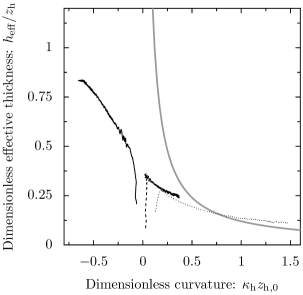
Figure 7.— Effective thickness of the photoevaporation flow on the $z$-axis versus heating front curvature. Lines represent models A (solid), B (dashed), and C (dotted). The thick gray line shows the expected relationship for a “globule” flow, $h=0.12/\kappa$.

Figure 7 graphs the dimensionless effective thickness against dimensionless curvature for all models and all times. It can be seen that the vast majority of points approximately follow a single curve for the three models. This is consistent with the idea that the flow thickness is controlled by the curvature of the ionization front. When the front is concave ($\kappa_{\mathrm{h}}<0$), the flow is not very divergent until it has passed the ionizing star, leading to a flow thickness of order the star-front distance. When one moves to flat and convex fronts, the flow divergence becomes more pronounced and its thickness becomes considerably less than the star-front distance. In the limit of large convex curvature ($\kappa_{\mathrm{h}}z_{\mathrm{h,0}}\gg 1$), then one would expect the flow to resemble that from a cometary globule (Bertoldi & McKee, 1990), with the flow thickness proportional to the radius of curvature: $h=\omega/\kappa$, where $\omega\simeq 0.12$. This curve is shown by the thick gray line in Figure 7 and it can be seen that our models are still some way from this regime.

3.4. Optical Line Emission

We have calculated the emissivity for three different types of line, representative of the strongest optical lines emitted by $\mathrm{H\,\scriptstyle II}$ regions. The first is a recombination line, such as the hydrogen Balmer lines, with emissivity

$$\eta_{\mathrm{rec}}(x)\propto n_{\mathrm{e}}n_{j+1}\,T^{-1},$$ (4)

where $n_{j+1}$ is the number density of the recombining ion, which we take to be proportional to $n_{\mathrm{i}}$. The second and third are both forbidden metal lines, excited by electron collisions, with emissivity

$$\eta_{\mathrm{col}}(x)\propto\frac{n_{\mathrm{e}}n_{j}}{\displaystyle 1+B_{\mathrm{col}}n_{\mathrm{e}}T^{-1/2}}\,\frac{e^{-E/kT}}{\sqrt{T}},$$ (5)

where $E$ is the excitation energy of the upper level, which we fix at $hc/6500\,\mathrm{\AA}$, and $B_{\mathrm{col}}$ is the collisional de-excitation coefficient, chosen to give a critical density of $1000\,\mathrm{cm^{-3}}$ at $10,000\,\mathrm{K}$. The second line is emitted by a neutral metal with $n_{j}\propto n_{\mathrm{n}}$, whereas the third line comes from an ionized metal with $n_{j}\propto n_{\mathrm{i}}$. Although the emissivities that we use are generic, they are each “inspired” by a particular optical emission line. In particular, the recombination line represents a hydrogen Balmer line such as H$\alpha$, the collisional neutral line represents [$\mathrm{O\,\scriptstyle I}$] 6300 Å, and the collisional ionized line represents a combination of [$\mathrm{N\,\scriptstyle II}$] 6584 Å and [$\mathrm{O\,\scriptstyle III}$] 5007 Å (since we do not consider the ionization of helium in our models, we cannot distinguish between singly and doubly ionized metals).

Figure 8.— Axial profiles of emissivity in different emission lines at an age of $78,000\,\mathrm{yr}$. The different models are shown by: A (solid line), B (dashed line), and C (dotted line). (a) Collisionally excited neutral metal line. (b) Collisionally excited ionized metal line. (c) Recombination line.

Figure 8 shows the emissivity of each line as a function of $z$ for each model, with arbitrary normalization. It can be seen that the neutral collisional line is confined to a thin region around the ionization front. This is because its emissivity contains a factor of $n_{\mathrm{e}}n_{\mathrm{n}}\propto x(1-x)$, which peaks at $x=0.5$. The other two lines show emissivity profiles that are broadly similar to one another since they are both proportional to $n_{\mathrm{i}}^{2}$. The differences between these two are mainly due to their different temperature dependences: the recombination line emissivity is relatively stronger at lower temperatures near the ionization front, while the collisional line is relatively stronger at higher temperatures, farther out in the flow. This behavior is further accentuated by the collisional deexcitation of the metal line, which reduces its strength at the higher densities found close to the ionization front.

Figure 9.— Simulated emission line profiles for a face-on viewing angle at an age of $78,000\,\mathrm{yr}$. The different models are shown by: A (solid line), B (dashed line), and C (dotted line). (a) Collisionally excited neutral metal line with atomic weight $A=16$. (b) Collisionally excited ionized metal line with $A=14$. (c) Recombination line with $A=1$.

We have also calculated the spectroscopic emission line profiles that would be seen by an observer looking along the $z$-axis. We assume that the radiative transfer can be calculated in the optically thin limit, in which case the emergent intensity profile is

$$I(u)=\int_{0}^{\infty}\eta(z)\,\exp\left[-\frac{\left(v(z)-u\right)^{2}}{2\Delta^{2}(z)}\right]\,dz,$$ (6)

where $u$ is the observed Doppler shift and $\Delta(z)$ is the thermal width at each point in the structure, which depends on the local sound speed and on the atomic weight, $A$, of the emitting species. The results are shown in Figure 9, assuming $A=1$ for the recombination line, $A=14$ for the ionized metal line, and $A=16$ for the neutral metal line.

The neutral metal line shows only a small blueshift ($\simeq 2\,\mathrm{km\,s^{-1}}$) of its peak with respect to the quiescent gas, but also has an extended blue wing. Its profile is almost indistinguishable between the different models. The ionized metal line shows the greatest variation between models but all are qualitatively similar with a large net blueshift (12–$17\,\mathrm{km\,s^{-1}}$) and a FWHM of $\simeq 10\,\mathrm{km\,s^{-1}}$, which is roughly double the thermal width. In cases in which the viewing angle has been determined by independent means, this line may be used to discriminate kinematically between the different models. The recombination line is also blueshifted (by about $10\,\mathrm{km\,s^{-1}}$) and again shows only slight variation between the models, with a FWHM that is now dominated by the thermal width because of the lower mass of H.

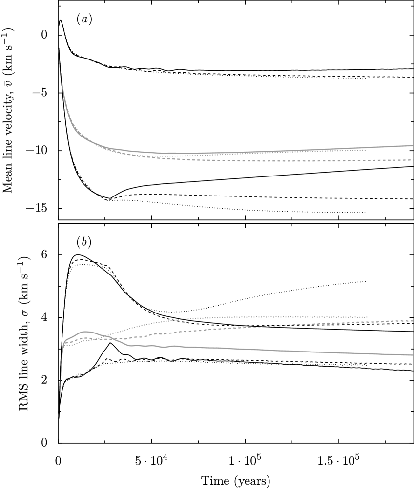
Figure 10.— Evolution of emission line kinematic properties for a face-on viewing angle for the three models. The different models are shown by: A (solid line), B (dashed line), and C (dotted line). (a) Mean line velocity, $\bar{v}$. (b) Root-mean-squared line width, $\sigma$. In panel (a), the top set of lines are for the neutral collisional line, the middle gray set are for the recombination line, and the bottom set are for the ionized collisional line. In the panel (b) the order is reversed.

The variation in the properties of the synthesized line profiles as the models evolve is presented in Figure 10, which shows the mean velocity,

$$\bar{v}=\frac{\displaystyle\int_{0}^{\infty}v(z)\eta(z)\,dz}{\displaystyle\int_{0}^{\infty}\eta(z)\,dz},$$ (7)

and the RMS velocity width,

$$\sigma=\frac{\displaystyle\int_{0}^{\infty}(v(z)-\bar{v})^{2}\eta(z)\,dz}{\displaystyle\int_{0}^{\infty}\eta(z)\,dz},$$ (8)

calculated for the three models as a function of time. Note that the velocity width, $\sigma$, only includes the contribution from the acceleration of the gas and does not include the thermal Doppler broadening. Supposing the emission to come predominantly from gas at $10^{4}\,\mathrm{K}$, the observed FWHM should be related to the RMS width by $\mathrm{FWHM}\simeq[(20\,\mathrm{km\,s^{-1}}/A)^{2}+(2.355\sigma)^{2}]^{1/2}$.

Once the models have settled down to their quasi-steady stage of evolution, it is remarkable how little variation is seen in the emission line properties, either between the models or as a function of time.

4. Observational parameters of the Orion Nebula

In this section, we derive observational parameters for the Orion nebula in order to compare with our simulations. We choose to use the spatial variation of the emission measure and electron density, together with the kinematic properties of various optical emission lines.

4.1. Emission measure and electron density

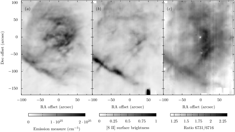
Figure 11.— (a) Emission measure. (b) [$\mathrm{S\,\scriptstyle II}$] 6716+6731 Å surface brightness. (c) [$\mathrm{S\,\scriptstyle II}$] $6731/6716$ ratio.

Emission measure and electron density maps of the inner Orion nebula are shown in Figure 11. We base these maps on velocity-resolved data cubes of the emissivity in various optical emission lines (García Díaz & Henney, 2003; Doi et al., 2004). This allows us to distinguish between the emission from the photoevaporation flow and that produced by Herbig-Haro shocks (O’Dell et al., 1997) and back-scattering from dust in the molecular cloud (Henney, 1998).

The emission measure map is calculated from the H$\alpha$ data of Doi et al. (2004), using a heliocentric velocity interval of $+1$ to $+33\,\mathrm{km\,s^{-1}}$, and correcting for foreground dust extinction using the $C(\mathrm{H\beta})$ map of O’Dell & Yusef-Zadeh (2000) and the extinction curve of Cardelli et al. (1989). The emission measure is assumed to be strictly proportional to the H$\alpha$ surface brightness, which would be the case for isothermal, Case B emission, and the constant of proportionality is found by comparison with the measured free-free optical depth at 20 cm (O’Dell & Yusef-Zadeh, 2000), assuming an electron temperature of $8900\,\mathrm{K}$. In regions of the map that do not contain significant high-velocity emission our derived emission measure is identical to that derived directly from the radio free-free data.

As an additional check on our results, we flux-calibrated our H$\alpha$ map (using the full velocity range) by comparison with published HST WFPC2 imaging (O’Dell & Doi, 1999; Bally et al., 2000) and converted to emission measure using the atomic parameters in Osterbrock (1989), which yielded values consistent at the 10% level with those derived by Baldwin et al. (1991) from the H 11–3 line. As recognised previously (Wen & O’Dell, 1995), the emission measures derived from the full velocity range of optical recombination lines are overestimated by up to 50% because of the contribution of light that has been back-scattered by dust in the molecular cloud. Our velocity-resolved technique automatically compensates for this without the need to introduce an arbitrary correction factor.

In order to calculate the electron density in the photoevaporation flow, we use velocity-resolved maps of the density-sensitive doublet lines [$\mathrm{S\,\scriptstyle II}$] 6716 and 6731 Å (García Díaz & Henney, 2003, 2005) to select only that gas in the range $+4$ to $+24\,\mathrm{km\,s^{-1}}$, close to the peak velocities of fully ionized species. The summed surface brightness in this velocity range for the two lines is shown in Figure 11b after correction for foreground extinction (the apparent emission peak at the lower right of the image is an artifact of the reduction procedure). The density-sensitive ratio $R=6731/6716$ for the same velocity range is shown in Figure 11c, in which higher values of $R$ correspond to higher densities. In order to calibrate our ratios, we first calculated maps summed over the full velocity range of the [$\mathrm{S\,\scriptstyle II}$] emission and compared these with the spectrophotometric data of Baldwin et al. (1991) and Pogge et al. (1992).

We find that a very good fit to the dependence of electron density on $R$ for gas at $8900\,\mathrm{K}$ (Cai & Pradhan, 1993) is

$$n_{\mathrm{e}}=n_{0}\frac{R-R_{1}}{R_{2}-R},$$ (9)

where $n_{0}=2489\,\mathrm{cm^{-3}}$, $R_{1}=0.697$, and $R_{2}=2.338$. Using this fit, the smallest ratio shown in Figure 11c corresponds to $n_{\mathrm{e}}\simeq 1000\,\mathrm{cm^{-3}}$ and the mid-range corresponds to 4–$6000\,\mathrm{cm^{-3}}$. The largest ratios shown in the image are in the high-density limit ($n_{\mathrm{e}}>10^{4}\,\mathrm{cm^{-3}}$), at which point the derived density becomes very uncertain due to the extreme sensitivity to experimental errors and variations in the temperature. Previous work, which did not resolve the kinematic line profiles, found that electron densities derived from fully ionized species (Jones, 1992; Megeath et al., 1990) are generally higher than those determined from [$\mathrm{S\,\scriptstyle II}$]. This has been attributed to the fact that part of the [$\mathrm{S\,\scriptstyle II}$] emission comes from partially ionized zones in which the electron fraction is significantly less than unity. As a result, it was found necessary to apply a correction factor to the [$\mathrm{S\,\scriptstyle II}$] densities, although there has been significant disagreement on its value (Baldwin et al., 1991; Wen & O’Dell, 1995). By using only the blue-shifted portion of the line profiles to calculate our densities, we are selecting the [$\mathrm{S\,\scriptstyle II}$] emission from the fully ionized gas. As a result, we have no need to apply a correction factor to our densities. Indeed we find that the $6731/6716$ ratio for the blue-shifted velocity range is typically 10% larger than the ratio calculated for the entire line, although there are some local variations and the difference is less at greater projected distances from the ionizing star.

4.2. Gas kinematics

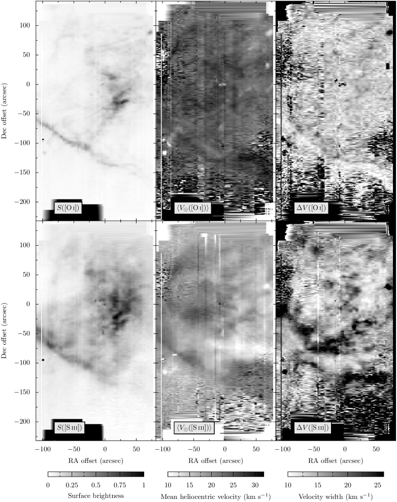
Figure 12.— Emission line maps for [$\mathrm{O\,\scriptstyle I}$] 6300 Å (top row) and [$\mathrm{S\,\scriptstyle III}$] 6312 Å (bottom row) constructed from longslit echelle spectroscopy. Left panels show the surface brightness. Central panels show the mean heliocentric line velocity. Right panels show the FWHM line width corrected for thermal and instrumental broadening.

In order to compare with the gas-kinematic behavior of the numerical models, we here present kinematic maps of the optical emission lines [$\mathrm{O\,\scriptstyle I}$] 6300 Å and [$\mathrm{S\,\scriptstyle III}$] 6312 Å (Figure 12). These are derived from echelle spectroscopy through a NS-oriented slit at a series of 60 different pointings using the Mezcal spectrograph of the Observatorio Astronómico Nacional, San Pedro Mártir, México. The observations are described in more detail in García Díaz & Henney (2005). We use these data in preference to the [$\mathrm{N\,\scriptstyle II}$], H$\alpha$, and [$\mathrm{O\,\scriptstyle III}$] data of Doi et al. (2004) because the latter contain no information on the east-west variation of the line velocities since they assume that the peak velocity of the total profile summed over each NS slit is the same. With our data, on the other hand, we have taken a pair of EW-oriented slit spectra, which allow us to “tie together” the wavelength calibrations of the individual NS slits. In addition, the existence in our spectra of the night-sky component to the [$\mathrm{O\,\scriptstyle I}$] line (at rest in the geocentric frame) allows us to make a very accurate wavelength calibration for that line. The images in Figure 12 show the spatial variation in line surface brightness (which has not been corrected for foreground extinction), the intensity-weighted mean line velocity, and the non-thermal component of the full-width half-maximum (FWHM) of the line, which was calculated by the subtraction in quadrature from the observed width of the instrumental width ($9\,\mathrm{km\,s^{-1}}$) and the thermal width ($5.35\,\mathrm{km\,s^{-1}}$ for [$\mathrm{O\,\scriptstyle I}$], $3.78\,\mathrm{km\,s^{-1}}$ for [$\mathrm{S\,\scriptstyle III}$]). All quantities were calculated for a spectral window that extends between heliocentric velocities of $-12$ to $+40\,\mathrm{km\,s^{-1}}$ to minimize the contamination from high-velocity emission from shocks.

The [$\mathrm{O\,\scriptstyle I}$] line is an example of a neutral collisional line, as discussed in § 3.4. As such, it originates in a thin zone close to the ionization front and shows a lot of fine-scale structure in its surface brightness. The mean velocity of [$\mathrm{O\,\scriptstyle I}$] is only blueshifted by a few $\mathrm{km\,s^{-1}}$ with respect to the molecular gas, which emits at $25$–$28\,\mathrm{km\,s^{-1}}$ (Omodaka et al., 1994; Wilson et al., 2001). There is a general trend for the [$\mathrm{O\,\scriptstyle I}$] emission to become more blue-shifted towards the west of the Trapezium, which is also seen in CO emission from the molecular gas (Wilson et al., 2001). Some of the bright linear filaments seen in the surface brightness map (such as the Bright Bar in the SW) correspond to filaments of increased redshift in the mean velocity map. Other linear structures in the mean velocity have no visible counterpart in the surface brightness (García Díaz & Henney, 2005). The most redshifted [$\mathrm{O\,\scriptstyle I}$] comes from diffuse emission just above the SE end of the Bright Bar, while the most blueshifted is due to the residual effect of high-velocity shocked emission from HH 201, 202, 203, and 204. The [$\mathrm{O\,\scriptstyle I}$] line width shows little large scale structure, with the notable exception of a marked decrease in the line width along the Bright Bar filament. Localized spots of increased line width correspond to the HH objects discussed above.

For the ionization parameter and EUV spectrum relevant to Orion, the [$\mathrm{S\,\scriptstyle III}$] emission traces the fully ionized gas ($x>0.9$), except for the zone closest to the ionizing star, which is predominantly S³⁺. It comes from a thicker layer and so shows smoother variations in surface brightness than does [$\mathrm{O\,\scriptstyle I}$], being similar in appearance to the emission measure map of Figure 11. The mean line velocity is blue-shifted several $\mathrm{km\,s^{-1}}$ with respect to [$\mathrm{O\,\scriptstyle I}$] and shows a more pronounced gradient from east to west. On the other hand, the large-scale features of the mean velocity map are rather similar to [$\mathrm{O\,\scriptstyle I}$], with redder emission being associated with the emission from the Bright Bar and other linear features. One feature seen in [$\mathrm{S\,\scriptstyle III}$] but not in [$\mathrm{O\,\scriptstyle I}$] is an EW-oriented spur of blue-shifted emission to the north of the Bright Bar (the $\mathrm{O\,\scriptstyle III}$ counterpart of this feature is discussed in Doi et al., 2004). The average [$\mathrm{S\,\scriptstyle III}$] linewidth is not much different from that of [$\mathrm{O\,\scriptstyle I}$] but [$\mathrm{S\,\scriptstyle III}$] shows much more variation across the nebula. The highest widths ($15$–$20\,\mathrm{km\,s^{-1}}$) are seen near the Trapezium, at the east end of the blue spur, and in the red-shifted emission at the faint SW end of the Bright Bar. The lowest widths ($\simeq 12\,\mathrm{km\,s^{-1}}$) are seen along the length of the Bright Bar and in a ring of radius 30–$60^{\prime\prime}$ around the Trapezium.

5. Application of the models to Orion

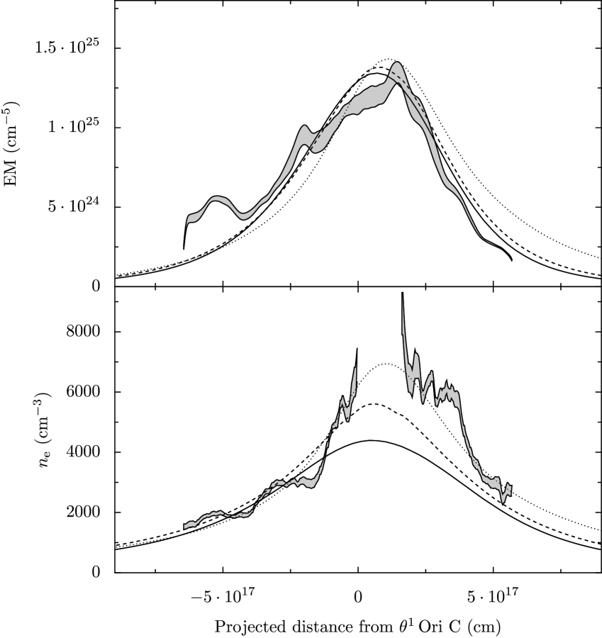
Figure 13.— Observed East-West profiles of emission measure (top panels) and electron density (bottom panels) in the Orion nebula (gray line), compared with predictions of the model simulations for an inclination angle of $15\arcdeg$: Model A (solid line), B (dashed line), and C (dotted line).

In order to compare our numerical simulations with the observational data of the previous section, we first extract the observational data in an EW strip, centered on the ionizing star $\theta^{1}$ Ori C. The strip is 60″ wide in the NS direction and the average emission measure (calculated from the H$\alpha$ surface brightness) and electron density (calculated from the [$\mathrm{S\,\scriptstyle II}$] line ratios) are shown in Figure 13 as a function of projected distance from the ionizing star (assuming a distance of 430 pc, O’Dell (2001b)). The data are represented by a gray band that indicates $\pm 3\sigma$ variation of individual pixels from the mean. The derived electron density is very uncertain close to $\theta^{1}$ Ori C on the West side since the observed line ratio is close to the high-density limit. We have therefore omitted this data from the graph.

We use the three models A, B, and C at a common age of $78,000\,\mathrm{yr}$ as representative of our numerical results and calculate the simulated observed profiles of emission measure and electron density for a viewing angle of $15\arcdeg$ with respect to the line of sight, following a procedure as close as possible to that employed in calculating the observed maps above. For the simulated emission measure, we first calculate simulated H$\alpha$ maps, restricted to the line-of-sight velocity range $-4$ to $-23\,\mathrm{km\,s^{-1}}$, then convert this to emission measure by assuming a fixed H$\alpha$ emissivity corresponding to $8900\,\mathrm{K}$. For the electron density, we calculate simulated maps for the $6716\,\mathrm{\AA}$ and $6731\,\mathrm{\AA}$ [$\mathrm{S\,\scriptstyle II}$] doublet components using the methods of § 3.4 for the same line-of-sight velocity range as for H$\alpha$. We then use the ratio of these two maps to derive $n_{\mathrm{e}}$ in exactly the same way as for the observations.

For each model, we rescale the lengths and densities to the Orion values as follows: first, we determine the star-ionization front distance, $z_{\mathrm{h,0}}$, by comparing the FWHM of the width of the EM in model units with the observed value of $6.12\times 10^{17}\,\mathrm{cm}$. Then, we determine the electron density scaling by fitting by eye to the broad peak of the observed EM profile.

The results are shown in the upper panel of Figure 13 in which it can be seen that all three models can provide a reasonable fit to the emission measure profile for a viewing angle of $15\arcdeg$. Models A and B fit the large-scale skewness of the profile somewhat better than Model C, which overpredicts the EM on the West side and underpredicts it on the East side. None of the models can reproduce the fine-scale structure seen in the observed profile. In general, the agreement is better on the West side of the profile, which is smoother than the East side. Model profiles for a viewing angle of $30\arcdeg$ (not shown) badly fail to fit the observed profile since their peaks are shifted too far to the West, while those for a viewing angle of $0\arcdeg$ (not shown) do not fit as well as the $15\arcdeg$ profiles since they are too symmetrical.

The parameters for the model fits in the $15\arcdeg$ case are listed in Table 1. These are the required effective ionizing photon luminosity of the central star, the distances along the symmetry axis from the star to the heating front and to the peak in the ionized gas density (see § 2), and the value of the ionized density peak. Since dust grains in the ionized nebula will absorb a fraction, $f_{\mathrm{d}}\sim 0.5$, of the ionizing photons emitted by the star (Arthur et al., 2004), and this effect is not included in the simulations, the derived quantity is $(1-f_{\mathrm{d}})Q_{\mathrm{H}}$.

Table 1Model fit parameters for $15\arcdeg$ viewing angle

	$(1-f_{\mathrm{d}})Q_{\mathrm{H}}/10^{49}\,\mathrm{s}^{-1}$	$z_{\mathrm{h,0}}/10^{17}\,\mathrm{cm}$	$z_{\mathrm{p,0}}/10^{17}\,\mathrm{cm}$	$n_{\mathrm{p}}/10^{4}\,\mathrm{cm^{-3}}$
Model	(1)	(2)	(3)	(4)
A	0.299	4.42	3.80	0.707
B	0.363	3.88	3.55	1.108
C	0.919	4.93	4.65	1.411

(1) Effective stellar ionizing luminosity. (2) Distance from star to heating front. (3) Distance from star to density peak. (4) Peak ionized density.

The results for the simulated observed electron density are shown in the lower panel of Figure 13 where it can be seen that Model C does the best job of fitting the observations. The other two models significantly underpredict the density in the central and Western portions of the nebula. None of the models reproduce the very high (but poorly determined) densities that seem to be indicated to exist close to $\theta^{1}$ Ori C. In § 6.1.3 below, we discuss how the the geometry of Model C can be reconciled with the fact that the nebula appears concave on the largest scales.

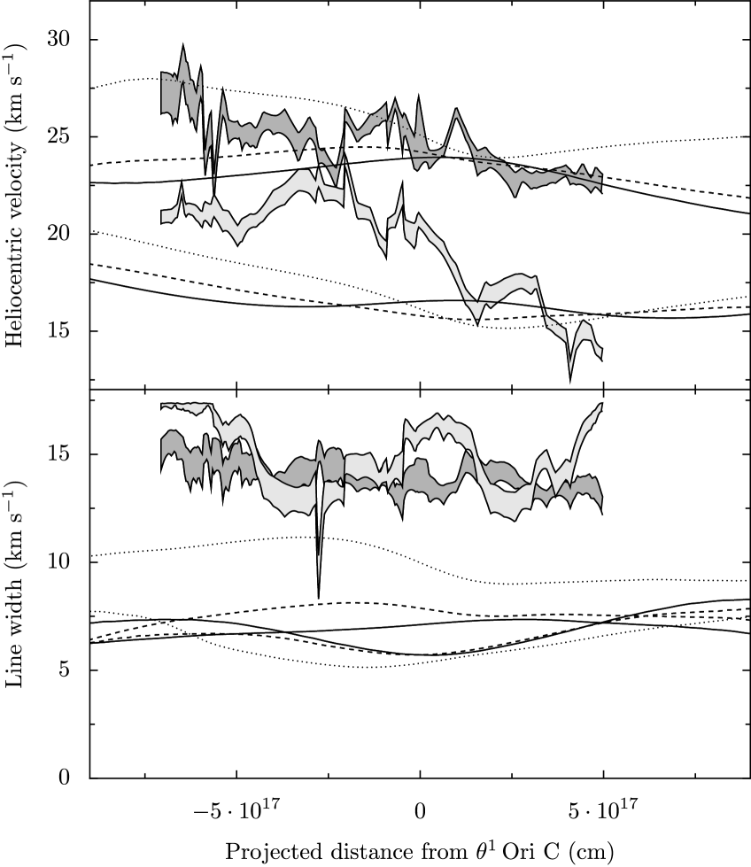
Figure 14.— Observed East-West profiles of [$\mathrm{O\,\scriptstyle I}$] (mid gray band) and [$\mathrm{S\,\scriptstyle III}$] (light gray band) mean velocity (top panels) and FWHM (bottom panels) in the Orion nebula, compared with predictions of the model simulations: Model A (solid line), B (dashed line), and C (dotted line).

We have also calculated simulated maps of mean velocity and line width of the [$\mathrm{O\,\scriptstyle I}$] and [$\mathrm{S\,\scriptstyle III}$] lines in order to compare with the observed kinematics presented in § 4.2. The results are shown in Figure 14 for the same EW strip as was used for the emission measure and density comparisons. The upper panel shows the observed mean heliocentric velocities of the two lines as gray bands indicating $\pm 3\sigma$ variation of individual pixels at each RA. The lines show the model predictions for an inclination angle of $15\arcdeg$ and assuming that the molecular gas has a constant heliocentric velocity of $+28\,\mathrm{km\,s^{-1}}$. The lower panel shows the same but for the non-thermal FWHM of the lines.

The models reproduce the magnitude and trend of the [$\mathrm{O\,\scriptstyle I}$] velocity as well as the qualitative fact that the [$\mathrm{S\,\scriptstyle III}$] is more blue-shifted than [$\mathrm{O\,\scriptstyle I}$]. Although they agree with the [$\mathrm{S\,\scriptstyle III}$] mean velocity on the western side of the nebula, they somewhat overpredict the blueshift of the [$\mathrm{S\,\scriptstyle III}$] line in the center of the nebula. Overall, Model C is a closer fit than the other models.

With regard to the line widths, the agreement is not very good. The observed [$\mathrm{S\,\scriptstyle III}$] widths are $2$–$5\,\mathrm{km\,s^{-1}}$ larger than the best model predictions (from Model C) and the [$\mathrm{O\,\scriptstyle I}$] widths are $7$–$9\,\mathrm{km\,s^{-1}}$ larger than any of the model predictions.

6. Discussion

6.1. The Orion Nebula

In § 5 the model predictions for the profiles of emission measure, electron density, and line kinematic properties are compared with observations of the Orion nebula. The EM profile is used to calibrate the length and density scales of the models and so its comparison with the model profiles does not provide a strong test. It is worth noting, however, that Models A and B can reproduce the large-scale skewness of the EM profile for a viewing angle of $15\arcdeg$, whereas Model C cannot. For Model C to produce the observed skewness requires a larger viewing angle, which shifts the predicted EM peak much farther to the West of $\theta^{1}$ Ori C than is observed. A further discrepancy with all the models is that the observed profile shows much fine-scale structure that is entirely absent in the simulations.

Since the observed $n_{\mathrm{e}}$ profile was not used in determining the model parameters, it provides a much more stringent test for the models. Only Model C predicts a sufficently high density in the central and Western regions of the nebula. Again, the observations show structure on scales $\leq 10^{17}\,\mathrm{cm}$, which are not present in the models.

6.1.1 Required ionizing photon luminosity

The derived parameters from the model fits (Table 1) show striking differences between the three models. In particular, the required effective ionizing photon luminosity is $Q_{\mathrm{H}}(1-f_{\mathrm{d}})=9.2\times 10^{48}\,\mathrm{s^{-1}}$ for Model C (where $f_{\mathrm{d}}$ is the fraction of ionizing photons absorbed by dust), which is roughly three times higher than the equivalent values for Models A and B. This is partly because the ionized density is more concentrated at the ionization front in Model C and thus requires a higher ionizing luminosity to sustain the same emission measure as compared to a situation in which the ionized gas is more evenly distributed between the star and the ionization front, as is the case for Models A and B. Another contributing factor is that the convexity of the ionization front of Model C (see Figure 3) means that the nebula is density-bounded for a large fraction of the solid angle as seen from the central star, whereas Models A and B are more concave and thus more ionization bounded. It has long been known that neutral gas in the so-called “veil” overlays the Orion nebula (van der Werf & Goss, 1989; Abel et al., 2004), so that the nebula must be ionization bounded on a scale of a few parsecs, thus contributing a low surface-brightness halo to the ionized emission. However, this would make a negligible contribution to the brightness of the inner region studied here. Indeed, Felli et al. (1993) find the total effective ionizing luminosity driving the nebula to be $9\times 10^{48}\,\mathrm{s^{-1}}$ from single-dish radio observations, which are sensitive to emission on a scale of parsecs that is not detected by interferometers. This is fully consistent with Model C but not with the other two models. Another independent estimate of the stellar ionizing luminosity comes from studying the surface brightness of the cusps of the Orion proplyds (Henney & Arthur, 1998; Henney & O’Dell, 1999), which gives a value of $(1-f^{\prime}_{\mathrm{d}})Q_{\mathrm{H}}=(1.0\pm 0.2)\times 10^{49}\,\mathrm{s^{-1}}$ for proplyd 167-317 (LV 2) that has the best-determined parameters (Henney et al., 2002). The fraction of ionizing photons absorbed by dust in the proplyd flow, $f^{\prime}_{\mathrm{d}}$, should be similar that for the nebula as a whole, $f_{\mathrm{d}}$, since in both cases the dust optical depth through the ionized gas is of order unity, so this result is also consistent only with our Model C.

6.1.2 Emission line kinematics and broadening

The comparison between the predicted and observed line kinematics is only partially successful. On the one hand, the trend of increasing blueshift with ionization is well reproduced by the models. This is a vast improvement on the plane-parallel weak-D models presented in Henney et al. (2005), which were unable to produce a difference of more than $1\,\mathrm{km\,s^{-1}}$ between the neutral and fully ionized lines. Our photoevaporation models predict a difference of about $5\,\mathrm{km\,s^{-1}}$ between [$\mathrm{O\,\scriptstyle I}$] and [$\mathrm{S\,\scriptstyle III}$], which is very similar to what is observed. The observations show a shift in the mean velocity from E to W of $\simeq 3\,\mathrm{km\,s^{-1}}$ for [$\mathrm{O\,\scriptstyle I}$] and $\simeq 6\,\mathrm{km\,s^{-1}}$ for [$\mathrm{S\,\scriptstyle III}$], which are both approximately reproduced by the models. In the case of [$\mathrm{O\,\scriptstyle I}$], some part of this variation can be accounted for by shifts in the velocity of the molecular gas behind the ionization front (Wilson et al., 2001) and furthermore the westernmost portion of the [$\mathrm{S\,\scriptstyle III}$] is affected by intermediate-velocity gas associated with the HH 202 jet and bowshock. Taking these into account, Model C can be seen to fit the observations quite well, apart from in the region around the Trapezium where the observed [$\mathrm{S\,\scriptstyle III}$] velocity is about $4\,\mathrm{km\,s^{-1}}$ redder than the model prediction. This may be evidence for the interaction of the stellar wind from $\theta^{1}$ Ori C with the photoevaporation flow, as is discussed further below.

On the other hand, the discrepancy seen between the predicted and observed line widths is very striking, especially for [$\mathrm{O\,\scriptstyle I}$], for which the models all predict a FWHM of $7\,\mathrm{km\,s^{-1}}$, which is only half the observed value. For [$\mathrm{S\,\scriptstyle III}$], the discrepancy, although less, is still significant: the best model predicts a FWHM of $12\,\mathrm{km\,s^{-1}}$ whereas the observed values range from $13$ to $17\,\mathrm{km\,s^{-1}}$. Since the widths of independent broadening agents should add approximately in quadrature, we thus require an extra broadening of $12\,\mathrm{km\,s^{-1}}$ for [$\mathrm{O\,\scriptstyle I}$] and $9\,\mathrm{km\,s^{-1}}$ for [$\mathrm{S\,\scriptstyle III}$]. The line widths in the models are mainly determined by the physical velocity gradients, $dv/dz$, in the photoevaporation flow and are of magnitude $\sim\left|dv/dz\right|\delta z$, where $\delta z$ is the thickness of the emitting layer. In principle, an additional broadening agent could be variation along the line of sight of the direction of the flow velocity vector (with magnitude $\sim\left|v\right|\delta\theta$) but this effect is very small in our models since the radius of curvature of the ionization front is of order the size of the nebula, so $\delta\theta$ is small. This broadening would be much more important if the ionization front had many small-scale irregularities, which does seem to be indicated by the large amount of structure seen in the surface brightness maps (Hester et al., 1991; O’Dell et al., 1991, 2003). An example of where this effect has been shown to be important is in the flows from the Orion proplyds (Henney & O’Dell, 1999). These are poorly resolved spatially with ground-based spectroscopy, so the full range of angles is present and one predicts line widths of order $2\left|v\right|$, with photoevaporation models successfully reproducing the observed line profiles for fully ionized species. However, although this small-scale divergence broadening might plausibly explain the [$\mathrm{S\,\scriptstyle III}$] linewidth discrepancy, it is hard to see how it can work for [$\mathrm{O\,\scriptstyle I}$] since the magnitude of the velocity in the [$\mathrm{O\,\scriptstyle I}$]-emitting zone is only $2$–$3\,\mathrm{km\,s^{-1}}$, which, even when doubled, is much smaller than the required broadening of $12\,\mathrm{km\,s^{-1}}$. Similar arguments apply to the contribution to the observed widths of back-scattered emission from dust behind the emitting layer (Henney, 1998), which again may be important for blueshifted lines such as [$\mathrm{S\,\scriptstyle III}$] but will be unimportant for [$\mathrm{O\,\scriptstyle I}$].

Previous authors have reached similar conclusions about the need for an extra broadening agent in the nebula from a purely empirical viewpoint (see O’Dell, 2001b, § 3.4.2–4 and references therein). More recently, O’Dell et al. (2003) have found evidence that the extra broadening may be greater in recombination lines than in collisional lines and thus may be related to the equally puzzling problem of temperature variations in the nebula.

Another proposed solution is that the broadening is caused by Alfvén waves, as is believed to be the case in giant molecular clouds (Myers & Goodman, 1988). In order to give an Alfvén velocity ($v_{\mathrm{a}}=\left(B^{2}/4\pi\rho\right)^{1/2}$) of $9\,\mathrm{km\,s^{-1}}$, which is necessary to explain the observed [$\mathrm{O\,\scriptstyle I}$] broadening, one requires a magnetic field of order $B=0.5\,\mathrm{mG}$ in the region where the line forms (which has an ionization fraction of order 20% and a total gas density roughly 3 times the peak ionized density). This is marginally inconsistent with the upper limit on $B$ derived from the Faraday rotation measure (Rao et al., 1998) and, furthermore, would predict very high Alfvén speeds either in the dense molecular gas or in the lower density, highly ionized gas. To see this, consider two possibilities for how the magnetic field responds to compression/rarefaction: first, suppose that $B$ is constant, such as might be the case for a highly ordered field with orientation parallel to the flow direction (perpendicular to the ionization front). In this case, $v_{\mathrm{A}}\sim\rho^{-1/2}$ and so a reasonable value is obtained in the dense molecular gas ($v_{\mathrm{A}}\simeq 3\,\mathrm{km\,s^{-1}}$ at $10^{5}\,\mathrm{cm^{-3}}$) but a very high value is obtained in the more highly ionized, lower density regions of the flow ($v_{\mathrm{A}}\simeq 30\,\mathrm{km\,s^{-1}}$ at $10^{3}\,\mathrm{cm^{-3}}$), which is ruled out by observations of lines such as [$\mathrm{O\,\scriptstyle III}$]. Second, suppose that $B$ is tangled or chaotic and can be considered as an isotropic pressure with effective adiabatic index $\gamma_{\mathrm{m}}=4/3$ (see Henney et al., 2005, Appendix C). In this case, $v_{\mathrm{A}}\sim\rho^{(\gamma_{\mathrm{m}}-1)/2}\sim\rho^{1/6}$, so that the Alfvén speed would have to exceed $10\,\mathrm{km\,s^{-1}}$ in the molecular gas, which greatly exceeds the linewidths of the molecular lines. Although we cannot definitely rule out the role of Alfvén waves, these considerations suggest that they do not provide a natural explanation for the line broadening.

6.1.3 Consistency with the large-scale nebular geometry

(a)(b)

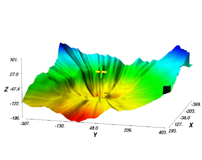
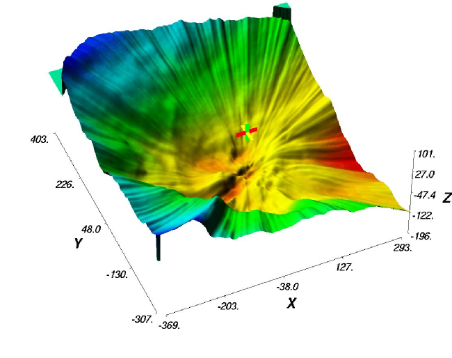
Figure 15.— Three-dimensional shape of the principal ionization front in Orion, derived from radio free-free surface brightness (Henney, 2005). (a) View over the molecular ridge from the WNW direction. (b) View over the Bright bar from the SSE direction. The $x$, $y$, and $z$ axes correspond to displacements along the EW, NS, and line-of-sight directions, respectively, with numerical values marked in arcseconds ($1^{\prime\prime}=6.45\times 10^{15}\,\mathrm{cm}$). The ionizing star is at the origin and is marked by a cross, while the observer is at $(x,y,z)=(0,0,+\infty)$. Shading of the surface indicates the $z$ height from low (red) to high (blue). This figure is available in color in the online edition.

Comparison of our models with the observed electron densities and line velocities in the nebula strongly favor Model C over the other two models, so it is worth considering whether the shape of the ionization front in this model is consistent with independent determinations. In Model C, the ionization front has a positive curvature, that is, it is convex as seen from the ionizing star. However, three-dimensional reconstruction of the shape of the ionization front paints a somewhat more complex picture (Wen & O’Dell, 1995; Henney, 2005), as is shown in Figure 15. In the brightest part of the nebula, just to the W of the ionizing star, the ionization front is indeed locally convex in the EW direction but is roughly flat in the NS direction. Also, the axis between the star and the closest point on the front is inclined at about $15\arcdeg$ to the line of sight, consistent with what we found for our models. On a larger scale, however, the front becomes concave in all directions apart from the south-west. The implications for our models are twofold: first, on a medium scale ($<1\arcmin\simeq 4\times 10^{17}\,\mathrm{cm}$) the flow should not be strictly cylindrically symmetric but instead should resemble Model C in its EW cross-section but more resemble Model B in its NS cross-section. Since we compared our models against an EW strip of the nebula, it is reasonable that Model C produced better fits. Secondly, on a larger scale the flow should come to more resemble Model A, but with a symmetry axis that is inclined towards the south-west, rather than towards the east and possible at a greater angle to the line-of-sight. How the flow will adjust between the differing curvature and symmetry axes is unclear, but it may involve internal shocks. Further complications will arise due to the interaction of the global flow with local flows from other convex features in the ionization front. The largest and most prominent of these is the Bright Bar but there are many other examples (O’Dell & Yusef-Zadeh, 2000), some of which are apparent in Figure 15.

6.2. Shortcomings of our models

Although our photoevaporation flow models have had some measure of success in accounting for the structure and kinematics of the Orion nebula on medium scales, there are many physical processes that we have neglected and which would need to be included in a complete model.

We have used a very simplified prescription for the radiative transfer in our models, in which we consider only one frequency for the ionizing radiation. Although we do include the hardening of the radiation field, thus accounting for the important reduction in the photoionization cross section deep in the ionization front, it would be more satisfactory to use a multi-frequency approach. The consideration of higher energy EUV radiation would allow us to calculate the helium ionization structure, while the inclusion of non-ionizing FUV radiation would permit a more realistic treatment of the heating and cooling in the neutral gas. Furthermore, the effects of dust absorption on the transfer of ionizing radiation are important and should be included.

One failure of our model has been an inability to acount for the reduced blueshift of high-ionization lines that is seen within a few times $10^{17}\,\mathrm{cm}$ of the Trapezium. It is possible that the stellar wind from $\theta^{1}$ Ori C or radiation pressure acting on dust grains may be important in this inner region. Both are effects that need to be incorporated in a future model.

There is much small scale structure present in the Orion ionization front (Hester et al., 1991), right down to scales $\sim 10^{15}\,\mathrm{cm}$, or smaller still if one includes the proplyds. Our models can be taken as reflecting the mean flow properties after all this small scale structure has been smeared out, but it is not obvious that such an approach is strictly valid. The very highest electron densities found close to the Trapezium are not reproduced by our models and seem to require that the emission there is dominated by much smaller-scale flows than we have considered. The effects of the mutual interaction of such flows is still in need of further research (but see Henney, 2003), which also needs to address the influence of bar-like features and the change in the orientation of the symmetry axis when one passes from $10^{18}\,\mathrm{cm}$ to $10^{19}\,\mathrm{cm}$ scales.

Lastly, but perhaps most importantly, our models completely neglect the role of the magnetic field. In the cold molecular gas, the pressure associated with magnetic field is expected to dominate the gas pressure, and so should have an important dynamic effect, but it is unclear if this is still the case in the ionized gas. For most plausible assumptions about the magnetic field geometry, the magnetic pressure is found to be a small fraction of the thermal pressure in the ionized gas (Henney et al., 2005). If the unexplained broadening of the [$\mathrm{O\,\scriptstyle I}$] line found in § 4.2 is ascribed to Alfvén turbulence, then this fraction may be as high as 25% at the ionization front. However, even if the magnetic field is dynamically unimportant in the ionized gas, it can still have an important effect on the jump conditions at the ionization front (Redman et al., 1998; Williams et al., 2000; Williams & Dyson, 2001).

7. Conclusions

We have carried out two-dimensional, cylindrically symmetric, hydrodynamical simulations of the photoevaporation of a cloud with large-scale density gradients, which gives rise to a transonic, ionized, photoevaporation flow with the following general properties:

1. After an initial transient phase, with duration $\sim 10^{4}\,\mathrm{yr}$ for typical compact $\mathrm{H\,\scriptstyle II}$ region sizes (§ 3.1), the flow enters a long-lived quasi-stationary phase in which the ionized flow is approximately steady in the frame of reference of the ionization/heating front (§ 3.2).

2. During the quasi-stationary phase (§§ 3.2, 3.3), the flow structure is determined entirely by two parameters: the distance of the ionizing star from the front, $z_{0}$, and the curvature of the front, $\kappa$. Depending on the curvature, the flows are more “champagne-like” ($\kappa<0$) or “globule-like” ($\kappa>0$).

3. The curvature of the front (§ 3.3) depends on the lateral density distribution in the neutral gas and on the evolutionary stage of the flow. Positively curved fronts are only obtained for lateral density distributions that are asymptotically steeper than $r^{-2}$. We found that initially flat or concave fronts tend to evolve with time towards more negative values of $\kappa z_{0}$ (increasing concavity), whereas initially convex fronts evolve towards more positive values of $\kappa z_{0}$ (increasing convexity).

4. The flat and convex ionization fronts in the simulations are found to be D-critical, whereas concave fronts are found to be weak-D (Appendix B). There is still a sonic point in the flows from concave fronts but it occurs in fully ionized gas, rather than in the front itself.

5. The relationship between gas ionization and kinematics shows little variation as a function of the front curvature (§ 3.4). In all cases, a gradient of $\simeq 10\,\mathrm{km\,s^{-1}}$ between the neutral and ionized gas is obtained. There is, however, a tendency for models with more positive curvature to show larger mean velocities and line widths for ionized species.

We have compared our models with both new and existing observations of the Orion nebula (§§ 4, 5), with the following results:

1. Only a convex model can simultaneously reproduce the observed distributions of emission measure and electron density in the nebula. A good fit is obtained for $\kappa z_{0}\simeq 0.5$, implying that the radius of curvature of the front is roughly twice its distance from the ionizing star. Flat and concave models predict an electron density in the west of the nebula that is much lower than is observed. They do, however, fit the observed emission measure distribution slightly better than a convex model.

2. Only a convex model is consistent with independent estimates of the ionizing luminosity, $Q_{\mathrm{H}}$, from $\theta^{1}$ Ori C. Flat and concave models trap a much higher fraction of the stellar ionizing photons in the central region of the nebula and predict a $Q_{\mathrm{H}}$ that is three times too small.

3. All the models can broadly reproduce the observed mean velocities of optical [$\mathrm{O\,\scriptstyle I}$] and [$\mathrm{S\,\scriptstyle III}$] emission lines but a convex model fits the data better.

4. None of the models can reproduce the observed widths of the optical emission lines, although convex models come close to doing so for the high-ionization lines. The largest discrepancy is found for the neutral [$\mathrm{O\,\scriptstyle I}$] line, which requires an extra broadening agent with a FWHM of $12\,\mathrm{km\,s^{-1}}$.

5. The best-fitting model over all has a flow axis inclined $15\arcdeg$ west from the line of sight and a distance between $\theta^{1}$ Ori C and the ionization front of $4.7\times 10^{17}\,\mathrm{cm}$.

Appendix A Analytic Model for the Flow from a Flat Ionization Front

In this section, we develop an approximate analytic treatment of the ionized portion of the photoevaporation flow, for the special case in which the ionization front is exactly flat. An earlier version of this calculation was presented in Henney (2003).

A.1. Assumptions and Simplifications

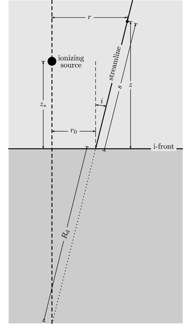
Figure 16.— Schematic diagram of the photoevaporation flow from a plane ionization front illuminated by a point source, in which the principal geometrical quantities are indicated.

Consider an infinite plane ionization front ($z=0$) illuminated by a point source of ionizing radiation, which lies at a height $z=z_{*}$ above the ionization front and defines the cylindrical axis $r=0$ (see Figure 16). Suppose that the ionization front is everywhere D-critical and that the volume $z>0$ is filled with a time-steady isothermal ionized photoevaporation flow with straight streamlines. Each streamline can be labeled with the cylindrical radius $r_{0}$ of its footpoint on the ionization front and makes an angle $i(r_{0})$ with the $z$-direction. Assume that the acceleration of the flow along a streamline is identical to that in the photoevaporation flow from a spherical globule with a radius equal to the local “divergence radius” of the flow: $R_{\mathrm{d}}=r_{0}\csc i$ so that the velocity along each streamline follows an identical function $U(y)\equiv u/c_{\mathrm{i}}$, where $y=1+s/R_{\mathrm{d}}$, $s$ is the distance along the streamline, and $c_{\mathrm{i}}$ is the isothermal sound speed in the ionized gas (since the front is D-critical, we have $U(0)=1$). The density at any point ($r$, $z$) can therefore be separated as

$$n(r,z)=\frac{N(r_{0})}{y^{2}U(y)}$$ (A1)

where $r=r_{0}+(y-1)R_{\mathrm{d}}\sin i$, $z=(y-1)R_{\mathrm{d}}\cos i$, and $N(r_{0})$ is the density at the ionization front.

The effective recombination thickness, $h$, is defined as in the caption to Figure 5, except integrated along a streamline rather than along the $z$-axis: $N^{2}(r_{0})h=\int_{0}^{\infty}n^{2}(r_{0},s)\,ds$, yielding

$$h=R_{\mathrm{d}}\int_{1}^{\infty}y^{-4}U^{-2}\,dy=\omega R_{\mathrm{d}},$$ (A2)

where $\omega$ is a constant that depends only on the acceleration law $U(y)$. Although $\omega\simeq 0.1$ is typical for spherical photoevaporation flows from globules (Bertoldi, 1989), the results of our numerical models above (see Fig. 7) suggest that the acceleration is somewhat slower in the present circumstances, leading to a larger value of $h$, so we leave $\omega$ as a free parameter for the time being.

A.2. Photoionization Balance

With this definition of $h$, and assuming that the photoevaporation flow is “recombination dominated” (Henney, 2001), that recombinations can be treated in the on-the-spot approximation, and ignoring any absorption of ionizing photons by grains, one can approximate the recombination/ionization balance along a line from the ionizing source to the ionization front by considering the perpendicular flux of ionizing photons incident on the equivalent homogeneous layer:

$$\frac{Q_{\mathrm{H}}\cos\theta}{4\pi(z_{*}^{2}+r_{0}^{2})}=\alpha_{\mathrm{B}}N^{2}(r_{0})h(r_{0}),$$ (A3)

where $\tan\theta=r_{0}/z_{*}$, $Q_{\mathrm{H}}$ is the ionizing photon luminosity (s^-1) of the source, and $\alpha_{\mathrm{B}}$ is the Case B recombination coefficient. This approximation will be valid when $h$ is small enough to satisfy $h<z_{*}$ and $h\sec\theta<H$, where $H\equiv\left|d\ln N/dr_{0}\right|^{-1}$ is the radial scale length of the ionized density profile at the ionization front. This profile can be found from equation (A3) to be

$$N(r_{0})=N_{0}\left(1+\frac{r_{0}^{2}}{z_{*}^{2}}\right)^{-3/4}\left(\frac{h}{h_{0}}\right)^{-1/2},$$ (A4)

where $x=r_{0}/z_{*}$ and $N_{0}$, $h_{0}$ are the values on the axis at $r_{0}=0$. Note that for any plausible $h(r_{0})$, the density at the ionization front will decrease with increasing radius.

A.3. Lateral Acceleration

In order to complete the solution, it is now only necessary to specify the radial dependence of the streamline angle, $i(r_{0})$, from which the radius of divergence, $R_{\mathrm{d}}(r_{0})$ and scale height, $h(r_{0})$, follow automatically. To do this, we must recognise that the streamlines cannot truly be straight: in a D-critical front the gas will be accelerated up to the ionized sound speed, $c_{\mathrm{i}}$, in the $z$-direction (perpendicular to the front) but at $z=0$ it will have no velocity in the $r$-direction (parallel to the front). However, the pressure gradient associated with the radially decreasing density will laterally accelerate the gas in the positive $r$-direction as it rises through the recombination layer (which is much thicker than the front itself), thus bending the streamlines outwards. To be definite, we will consider the characteristic angle of each streamline, $i(r_{0})$, to be that obtained by the gas at $z=h(r_{0})$.

The lateral acceleration, $a$, of the gas is given by

$$a=\frac{1}{\rho}\frac{dP}{dr}=\frac{c_{\mathrm{i}}^{2}}{H},$$ (A5)

where $H$ is the lateral density scale length defined above. Immediately after passing through the heating front, the gas will have a vertical velocity of $\simeq 0.3c_{\mathrm{i}}$, rising to $\simeq c_{\mathrm{i}}$ once it is fully ionized and then to $\simeq 2c_{\mathrm{i}}$ as it passes through the recombination layer. We take the typical vertical speed to be $v_{z}=\beta c_{\mathrm{i}}$, where $\beta$ is a parameter whose value must be determined but which should be somewhat less than unity. Hence, the time taken to rise to a height $h$ is $\delta t=h/\beta c_{\mathrm{i}}$, so that the lateral speed reached is $v_{r}=a\delta t=c_{\mathrm{i}}h/\beta H$ and the streamline angle is given by

$$\tan i=\frac{v_{r}}{v_{z}}=\frac{h}{\beta H},$$ (A6)

so that $R_{\mathrm{d}}=h/\omega=r_{0}(1+\beta^{2}H^{2}/h^{2})^{1/2}$ (see Fig. 16). In the limit that $h^{2}/\beta^{2}H^{2}\ll 1$, this can be solved to give

$$h\simeq(\omega\beta Hr_{0})^{1/2},$$ (A7)

which can be combined with equation (A4) and the definition of $H$ to give the following ODE for $h$:

$$\frac{dh}{dr_{0}}+\frac{3hr_{0}}{r_{0}^{2}+z_{*}^{2}}-\frac{2\omega\beta r_{0}}{h}=0.$$ (A8)

This can be solved directly by means of the substitution $y=h^{2}$ and the integrating factor $(r_{0}^{2}+z_{*}^{2})^{3}$ to give

$$h=\left(\frac{\omega\beta}{2}\right)^{1/2}z_{0}\left(1+\frac{r_{0}^{2}}{z_{*}^{2}}\right)^{1/2}$$ (A9)

which may in turn be substituted back into equation (A4) to give

$$N(r_{0})=N_{0}\left(1+\frac{r_{0}^{2}}{z_{*}^{2}}\right)^{-1}.$$ (A10)

From equation (A6), the streamline angles are then given by

$$\tan i=\left(\frac{\omega}{2\beta}\right)^{1/2}\frac{r_{0}}{\left(r_{0}^{2}+z_{*}^{2}\right)^{1/2}}.$$ (A11)

Hence, the vertical scale height on the axis is given by $h_{0}=(\omega\beta/2)^{1/2}z_{*}$, at which point the streamlines are vertical. We can now fix the value of $\omega\beta$ by comparing this with our numerical results from the model simulations. Figure 7 shows that for zero curvature, $h_{\mathrm{eff}}/z_{\mathrm{h}}\simeq 0.4$, which implies $\omega\beta\simeq 0.3$. Moving away from the axis, the streamlines start to diverge slightly, reaching an asympotic angle of $i_{\infty}=\tan^{-1}(\omega/2\beta)^{1/2}$ as $r_{0}\rightarrow\infty$. In Figure 17 this behavior of the streamline angle is compared with that seen in our numerical simulations of Model B, where it is found that $\omega/\beta\simeq 0.6$ gives a reasonable fit for $r_{0}<z_{*}$, which, combined with the estimate of $\omega\beta$, yields $\omega\simeq 0.4$ and $\beta\simeq 0.7$.

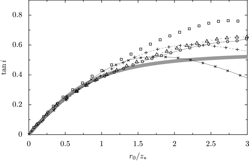
Figure 17.— Comparison of the increase in streamline angle with radius between the analytic model (thick gray line) and the numerical simulation of Model B at various evolutionary times: 40,000 (crosses), 60,000 (plusses), 80,000 (squares), 100,000 (circles), and 120,000 (triangles) years.

The validity of the analytical results for $r_{0}$ greater than a few times $z_{*}$ is not to be expected, since $h$ no longer satisfies the conditions stated after equation (A3) above. Nonetheless, it is satisfying that the general characteristics of the photoevaporation flows seen in our numerical simulations can be reproduced from these simple physical arguments.

It is interesting to consider how the calculation would be affected by the presence of dust grains in the ionized flow, which absorb part of the ionizing radiation. To first order, this may be treated by considering the column density of gas between the ionizing star and the ionization front, which is proportional to $Nh/\cos\theta$. From equations (A9) and (A10) it can be seen that this column density is a constant for all values of $r_{0}$. As a result, dust absorption has no differential effect on the structure of the flow in this approximation but merely reduces the effective ionizing luminosity of the star.

Appendix B Are the Ionization Fronts D-critical?

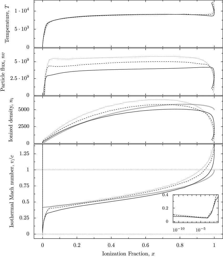
Figure 18.— Structure of the ionization front: various physical quantities as a function of ionization fraction, $x$. (a) Gas temperature. (b) Particle flux. (c) Ionized density. (d) Isothermal Mach number, with inset showing the same quantity on a logarithmic scale for small values of $x$. The different models are shown by: A (solid line), B (dashed line), and C (dotted line). The analytic curves of ionized density and Mach number for a steady, plane-parallel, isothermal, D-critical front are shown by thick gray lines. All velocities are given relative to the heating front.

The traditional classification of ionization fronts into weak/critical/strong and R-type/D-type (Kahn, 1954; Goldsworthy, 1961) was carried out for plane-parallel fronts. Although the fronts can be curved in our simulations, the ionization front thickness is always much less than the radius of curvature and so a plane-parallel approximation is justified for the front itself. It is therefore an interesting question whether or not our fronts are indeed D-critical, as is often assumed for photoevaporation flows.

Two approaches are possible to the empirical classification of the ionization fronts in the simulations. One possibility is to look at the velocity of propagation of the front with respect to the upstream gas. The other is to look at the internal structure of the front, which is the method we investigate first.

Figure 18 graphs various quantities as a function of ionization fraction, $x$. Figure 18a shows that almost all the gas heating in the front occurs at very low values of $x$, so the ionization transition itself can be considered approximately isothermal. Furthermore, Figure 18b shows that the particle flux is roughly constant through a great part of the front. At very low ionization fractions, the flow is not steady because the shock propagates at a slightly faster speed than the ionization front. At high ionization fractions, the streamlines start to diverge and the flow is no longer plane parallel, resulting in a reduction of the particle flux. Nonetheless, the flow can be seen to be approximately steady and plane-parallel over virtually the entire front.

In this case, one can apply the simple model developed in Appendix A of Henney et al. (2005). For a time-steady, plane-parallel, isothermal, D-critical front, where the critical point occurs at $x=1$, then the results of that paper imply

$$M(x)=\frac{2^{1/2}-(1-x)^{1/2}}{(1+x)^{1/2}}$$ (B1)

and

$$n_{\mathrm{i}}\propto\frac{x}{1-[(1-x)/2]^{1/2}}.$$ (B2)

These curves are shown in Figure 18c and d (thick gray lines), together with the same quantities for the three numerical models at an age of $78,000\,\mathrm{yr}$. The normalization of the theoretical $n_{\mathrm{i}}$ curve is arbitrary. The three models are very similar and also agree quite well with the analytical curve, except for near $x=0$ and $x=1$. In particular, the D-critical curve implies that the Mach number immediately after the heating front at $x\simeq 0$ should be $M_{\mathrm{h}}=\sqrt{2}-1\simeq 0.414$, which is close to that observed in the numerical models. This implies that the models are all close to D-critical, although they all pass through the sonic point before reaching $x=1$, with the most divergent model (C) doing so at $x\simeq 0.9$. Model A, which is the least divergent, shows a somewhat smaller initial jump in the Mach number, which may be evidence that it is weaker than D-critical.

The numerical models all show a maximum in the ionized density between $x=0.6$ and $x=0.8$, similar to that predicted by the D-critical curve. At higher values of $x$, on the other hand, the ionized density decreases much faster than in the analytical model because of the divergence in the numerical models. Note, however, that the particle flux is constant in the vicinity of the maxima in $n_{\mathrm{i}}$, so divergence is not important there.

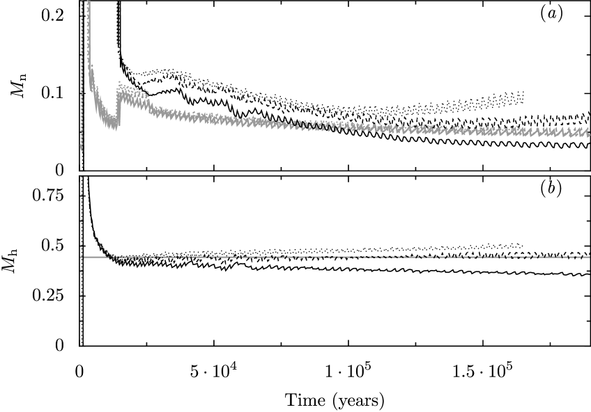
Figure 19.— Evolution with time of relative Mach numbers of the gas flow either side of the heating front. (a) Relative Mach number with which neutral gas enters the heating front, $M_{\mathrm{n}}$ (black lines). Also shown (gray lines) is the critical Mach number for a steady flow, $c_{\mathrm{n}}/2c_{\mathrm{i}}$. (b) Relative Mach number with which gas leaves the heating front, $M_{\mathrm{h}}$, calculated at $x=0.1$. Gray line shows the analytical approximation for a D-critical front.

The other test of the D-critical hypothesis is to look at the Mach number on the neutral side, that is, the Mach number of the gas flow relative to the heating front as it enters the front from the shocked neutral shell, $M_{\mathrm{n}}$. For a steady, plane-parallel front, there exists a maximum value, $M_{\mathrm{n,max}}=c_{\mathrm{n}}/2c_{\mathrm{i}}$, which corresponds to a D-critical front. $M_{\mathrm{n}}$ is about 0.06 for the models shown in Fig. 18d, as can be seen from the inset. The evolution with time of $M_{\mathrm{n}}$ for the models is shown in Figure 19a, which also shows (gray line) the theoretical maximum value, $M_{\mathrm{n,max}}$, taking $c_{\mathrm{i}}$ to be the sound speed at the sonic point in the flow. It can be seen that $M_{\mathrm{n}}$ actually exceeds $M_{\mathrm{n,max}}$ everywhere except for the late-time evolution of Model A! This should not be possible for a steady flow but is probably due to the fact that the sound speed in the neutral shell, $c_{\mathrm{n}}$, varies spatially within the shell, according to the past history of the propagation speed of the shock front, $U_{\mathrm{s}}$, thus violating the steady-state assumption even though the flow from the shell through the ionization front is approximately steady. Hence, $M_{\mathrm{n}}$ is not a suitable diagnostic for classifying the ionization front.

The evolution with time of $M_{\mathrm{h}}$ is shown in Figure 19b, calculated at the point where the gas leaves the heating front at $x=0.1$. At this point in the flow, the gas has already heated up to $\simeq 10^{4}\,\mathrm{K}$, although it is still largely neutral, see Figure 18. The analytic value for a D-critical front with a sonic point at $x=1$ is shown by the gray line (see eq.(B1) above). The numerical results for Model B can be seen to trace the analytical line almost exactly, indicating that the front is indeed D-critical in this model. For Model C, $M_{\mathrm{h}}$ slightly exceeds that analytical value, but this can be explained by the fact that the sonic point occurs nearer to $x=0.9$ in this model (see Fig. 18d). For Model A, $M_{\mathrm{h}}$ falls increasingly below the D-critical value as the evolution progresses, indicating that the ionization front becomes increasingly weak-D. This implies that there should be no sonic point within the ionization front itself. This is consistent with the fact that the sonic point occurs much further from the heating front than in the other two models (see Fig. 5c), in a region where the gas is fully ionized.

References

- Abel et al. (2004) Abel, N. P., Brogan, C. L., Ferland, G. J., O’Dell, C. R., Shaw, G., & Troland, T. H. 2004, ApJ, 609, 247
- Arthur et al. (2004) Arthur, S. J., Kurtz, S. E., Franco, J., & Albarrán, M. Y. 2004, ApJ, 608, 282
- Baldwin et al. (1991) Baldwin, J. A., Ferland, G. J., Martin, P. G., Corbin, M. R., Cota, S. A., Peterson, B. M., & Slettebak, A. 1991, ApJ, 374, 580 [ADS]
- Balick et al. (1974) Balick, B., Gammon, R. H., & Hjellming, R. M. 1974, PASP, 86, 616
- Bally et al. (2000) Bally, J., O’Dell, C. R., & McCaughrean, M. J. 2000, AJ, 119, 2919
- Bedijn & Tenorio-Tagle (1981) Bedijn, P. J. & Tenorio-Tagle, G. 1981, A&A, 98, 85
- Bedijn & Tenorio-Tagle (1984) —. 1984, A&A, 135, 81
- Bertoldi (1989) Bertoldi, F. 1989, ApJ, 346, 735
- Bertoldi & McKee (1990) Bertoldi, F. & McKee, C. F. 1990, ApJ, 354, 529
- Bodenheimer et al. (1979) Bodenheimer, P., Tenorio-Tagle, G., & Yorke, H. W. 1979, ApJ, 233, 85
- Cai & Pradhan (1993) Cai, W. & Pradhan, A. K. 1993, ApJS, 88, 329
- Cardelli et al. (1989) Cardelli, J. A., Clayton, G. C., & Mathis, J. S. 1989, ApJ, 345, 245
- Comeron (1997) Comeron, F. 1997, A&A, 326, 1195 [ADS]
- Doi et al. (2004) Doi, T., O’Dell, C. R., & Hartigan, P. 2004, AJ, 0, 0
- Dyson (1968) Dyson, J. E. 1968, Ap&SS, 1, 388
- Felli et al. (1993) Felli, M., Churchwell, E., Wilson, T. L., & Taylor, G. B. 1993, A&AS, 98, 137
- Ferland (2000) Ferland, G. J. 2000, in Astrophysical Plasmas: Codes, Models, and Observations, (Eds. S. J. Arthur, N. Brickhouse, and J. Franco) Revista Mexicana de Astronomía y Astrofísica (Serie de Conferencias), Vol. 9, 153–157 [ADS]
- Ferland (2001) Ferland, G. J. 2001, PASP, 113, 41 [ADS]
- Franco et al. (1989) Franco, J., Tenorio-Tagle, G., & Bodenheimer, P. 1989, Revista Mexicana de Astronomia y Astrofisica, vol. 18, 18, 65
- García Díaz & Henney (2003) García Díaz, M. T. & Henney, W. J. 2003, in Winds, Bubbles and Explosions, (Eds. S. J. Arthur and W. J. Henney) Revista Mexicana de Astronomía y Astrofísica (Serie de Conferencias), Vol. 15, 201–201
- García Díaz & Henney (2005) García Díaz, M. T. & Henney, W. J. 2005, ApJ, in preparation
- Garcia-Segura & Franco (1996) Garcia-Segura, G. & Franco, J. 1996, ApJ, 469, 171
- Godunov (1959) Godunov, S. K. 1959, Mat. Sbornik, 47, 271
- Goldsworthy (1961) Goldsworthy, F. A. 1961, Phil. Trans. A, 253, 277
- Henney (1998) Henney, W. J. 1998, ApJ, 503, 760 [ADS]
- Henney (2001) Henney, W. J. 2001, in The Seventh Texas-Mexico Conference on Astrophysics: Flows, Blows and Glows (Eds. William H. Lee and Silvia Torres-Peimbert) Revista Mexicana de Astronomía y Astrofísica (Serie de Conferencias) Vol. 10, pp. 57-60 (2001), 57–60 [ADS]
- Henney (2003) Henney, W. J. 2003, in Winds, Bubbles and Explosions, (Eds. S. J. Arthur and W. J. Henney) Revista Mexicana de Astronomía y Astrofísica (Serie de Conferencias), Vol. 15, 175–180
- Henney (2005) Henney, W. J. 2005, ApJ, xxx, xxx, in preparation
- Henney & Arthur (1998) Henney, W. J. & Arthur, S. J. 1998, AJ, 116, 322 [ADS]
- Henney et al. (2005) Henney, W. J., Arthur, S. J., Williams, R. J. R., & Ferland, G. J. 2005, ApJ, 621, 328
- Henney & O’Dell (1999) Henney, W. J. & O’Dell, C. R. 1999, AJ, 118, 2350 [ADS]
- Henney et al. (2002) Henney, W. J., O’Dell, C. R., Meaburn, J., Garrington, S. T., & Lopez, J. A. 2002, ApJ, 566, 315 [ADS]
- Hester et al. (1991) Hester, J. J., Gilmozzi, R., O’Dell, C. R., Faber, S. M., Campbell, B., Code, A., Currie, D. G., Danielson, G. E., Ewald, S. P., Groth, E. J., Holtzman, J. A., Kelsall, T., Lauer, T. R., Light, R. M., Lynds, R., O’Neil, E. J., Shaya, E. J., & Westphal, J. A. 1991, ApJ, 369, L75
- Hester et al. (1996) Hester, J. J., Scowen, P. A., Sankrit, R., Lauer, T. R., Ajhar, E. A., Baum, W. A., Code, A., Currie, D. G., Danielson, G. E., Ewald, S. P., Faber, S. M., Grillmair, C. J., Groth, E. J., Holtzman, J. A., Hunter, D. A., Kristian, J., Light, R. M., Lynds, C. R., Monet, D. G., O’Neil, E. J., Shaya, E. J., Seidelmann, K. P., & Westphal, J. A. 1996, AJ, 111, 2349
- Israel (1978) Israel, F. P. 1978, A&A, 70, 769
- Johnstone & Bally (1999) Johnstone, D. & Bally, J. 1999, ApJ, 510, L49 [ADS]
- Johnstone et al. (1998) Johnstone, D., Hollenbach, D., & Bally, J. 1998, ApJ, 499, 758 [ADS]
- Jones (1992) Jones, M. R. 1992, Ph.D. Thesis
- Kahn (1954) Kahn, F. D. 1954, Bull. Astron. Inst. Netherlands, 12, 187
- Kaler (1967) Kaler, J. B. 1967, ApJ, 148, 925
- López-Martín et al. (2001) López-Martín, L., Raga, A. C., Mellema, G., Henney, W. J., & Cantó, J. 2001, ApJ, 548, 288 [ADS]
- Megeath et al. (1990) Megeath, S. T., Herter, T., Gull, G. E., & Houck, J. R. 1990, ApJ, 356, 534
- Moore et al. (2002) Moore, B. D., Hester, J. J., Scowen, P. A., & Walter, D. K. 2002, AJ, 124, 3305 [ADS]
- Myers & Goodman (1988) Myers, P. C. & Goodman, A. A. 1988, ApJ, 326, L27
- O’Dell (2001a) O’Dell, C. R. 2001a, PASP, 113, 29
- O’Dell (2001b) —. 2001b, ARA&A, 39, 99 [ADS]
- O’Dell & Doi (1999) O’Dell, C. R. & Doi, T. 1999, PASP, 111, 1316 [ADS]
- O’Dell et al. (2001) O’Dell, C. R., Ferland, G. J., & Henney, W. J. 2001, ApJ, 556, 203 [ADS]
- O’Dell et al. (1997) O’Dell, C. R., Hartigan, P., Lane, W. M., Wong, S. K., Burton, M. G., Raymond, J., & Axon, D. J. 1997, AJ, 114, 730
- O’Dell et al. (2000) O’Dell, C. R., Henney, W. J., & Burkert, A. 2000, AJ, 119, 2910 [ADS]
- O’Dell et al. (2003) O’Dell, C. R., Peimbert, M., & Peimbert, A. 2003, AJ, 125, 2590
- O’Dell et al. (1993) O’Dell, C. R., Valk, J. H., Wen, Z., & Meyer, D. M. 1993, ApJ, 403, 678
- O’Dell et al. (1991) O’Dell, C. R., Wen, Z., & Hester, J. J. 1991, PASP, 103, 824
- O’Dell & Yusef-Zadeh (2000) O’Dell, C. R. & Yusef-Zadeh, F. 2000, AJ, 120, 382
- Omodaka et al. (1994) Omodaka, T., Hayashi, M., Hasegawa, T., & Hayashi, S. S. 1994, ApJ, 430, 256
- Osterbrock (1989) Osterbrock, D. E. 1989, Astrophysics of gaseous nebulae and active galactic nuclei (Mill Valley, CA: University Science Books)
- Pankonin et al. (1979) Pankonin, V., Walmsley, C. M., & Harwit, M. 1979, A&A, 75, 34
- Pogge et al. (1992) Pogge, R. W., Owen, J. M., & Atwood, B. 1992, ApJ, 399, 147
- Pottasch (1956) Pottasch, S. R. 1956, Bull. Astron. Inst. Netherlands, 13, 77
- Quirk (1994) Quirk, J. J. 1994, Internat. J. Numer. Methods Fluids, 18, 555
- Raga et al. (1999) Raga, A. C., Mellema, G., Arthur, S. J., Binette, L., Ferruit, P., & Steffen, W. 1999, Revista Mexicana de Astronomia y Astrofisica, 35, 123
- Rao et al. (1998) Rao, R., Crutcher, R. M., Plambeck, R. L., & Wright, M. C. H. 1998, ApJ, 502, L75+
- Redman et al. (1998) Redman, M. P., Williams, R. J. R., Dyson, J. E., Hartquist, T. W., & Fernandez, B. R. 1998, A&A, 331, 1099 [ADS]
- Rubin et al. (1991) Rubin, R. H., Simpson, J. P., Haas, M. R., & Erickson, E. F. 1991, ApJ, 374, 564
- Sanders et al. (1998) Sanders, R., Morano, E., & Druguet, M. 1998, J. Comp. Phys., 145, 511
- Sankrit & Hester (2000) Sankrit, R. & Hester, J. J. 2000, ApJ, 535, 847 [ADS]
- Scowen et al. (1998) Scowen, P. A., Hester, J. J., Sankrit, R., Gallagher, J. S., Ballester, G. E., Burrows, C. J., Clarke, J. T., Crisp, D., Evans, R. W., Griffiths, R. E., Hoessel, J. G., Holtzman, J. A., Krist, J., Mould, J. R., Stapelfeldt, K. R., Trauger, J. T., Watson, A. M., & Westphal, J. A. 1998, AJ, 116, 163 [ADS]
- Shu (1992) Shu, F. H. 1992, Physics of Astrophysics, Vol. II (University Science Books)
- Subrahmanyan et al. (2001) Subrahmanyan, R., Goss, W. M., & Malin, D. F. 2001, AJ, 121, 399 [ADS]
- Tenorio-Tagle (1979) Tenorio-Tagle, G. 1979, A&A, 71, 59
- Tenorio-Tagle & Bedijn (1981) Tenorio-Tagle, G. & Bedijn, P. J. 1981, A&A, 99, 305
- van der Werf & Goss (1989) van der Werf, P. P. & Goss, W. M. 1989, A&A, 224, 209
- van Leer (1982) van Leer, B. 1982, in Lecture Notes in Physics, Vol. 170, xxx, ed. E. Krause (Springer-Verlag), 507
- Vandervoort (1963) Vandervoort, P. O. 1963, AJ, 68, 296
- Vandervoort (1964) —. 1964, ApJ, 139, 869
- Wen & O’Dell (1995) Wen, Z. & O’Dell, C. R. 1995, ApJ, 438, 784
- Williams (1999) Williams, R. J. R. 1999, MNRAS, 310, 789 [ADS]
- Williams (2002) —. 2002, MNRAS, 331, 693 [ADS]
- Williams & Dyson (2001) Williams, R. J. R. & Dyson, J. E. 2001, MNRAS, 325, 293 [ADS]
- Williams et al. (2000) Williams, R. J. R., Dyson, J. E., & Hartquist, T. W. 2000, MNRAS, 314, 315 [ADS]
- Wilson et al. (2001) Wilson, T. L., Muders, D., Kramer, C., & Henkel, C. 2001, ApJ, 557, 240
- Yorke et al. (1982) Yorke, H. W., Bodenheimer, P., & Tenorio-Tagle, G. 1982, A&A, 108, 25
- Zuckerman (1973) Zuckerman, B. 1973, ApJ, 183, 863