Gravitational evolution of a perturbed lattice and its fluid limit

Abstract

We apply a simple linearization, well known in solid state physics, to approximate the evolution at early times of cosmological $N$-body simulations of gravity. In the limit that the initial perturbations, applied to an infinite perfect lattice, are at wavelengths much greater than the lattice spacing $l$ the evolution is exactly that of a pressureless self-gravitating fluid treated in the analagous (Lagrangian) linearization, with the Zeldovich approximation as a sub-class of asymptotic solutions. Our less restricted approximation allows one to trace the evolution of the discrete distribution until the time when particles approach one another (i.e. “shell crossing”). We calculate modifications of the fluid evolution, explicitly dependent on $l$ i.e. discreteness effects in the N body simulations. We note that these effects become increasingly important as the initial red-shift is increased at fixed $l$. The possible advantages of using a body centred cubic, rather than simple cubic, lattice are pointed out.

In current cosmological theories the physics of structure formation in the universe reduces, over a large range of scales, to understanding the evolution of clustering under Newtonian gravity, with only a simple modification of the dynamical equations due to the expansion of the Universe. The primary instrument for solving this problem is numerical $N$-body simulation (NBS, see e.g.nbs-standard-references ). These simulations are most usually started from configurations which are simple cubic (sc) lattices perturbed in a manner prescribed by a theoretical cosmological model. In this letter we observe that, up to a change in sign in the force, the initial configuration is identical to the Coulomb lattice (or Wigner crystal) in solid state physics (see e.g. pines ), and we exploit this analogy to develop an approximation to the evolution of these simulations. We show that one obtains, for long wavelength perturbations, the evolution predicted by an analagous fluid description of the self-gravitating system, and in particular, as a special case, the Zeldovich approximation zeldovich-ZApaper . Further we can study precisely the deviations from this fluid-like behaviour at shorter wavelengths arising from the discrete nature of the system. This analysis should be a useful step towards a precise quantitative understanding, which is currently lacking, of the role of discreteness in cosmological NBS (see e.g. discreteness-references ; discreteness-tbmjfsl ; discreteness-hamana ). One simple conclusion, for example, is that a body centred cubic (bcc) lattice may be a better choice of discretisation, as its spectrum has only growing modes with exponents bounded above by that of fluid linear theory.

The equation of motion of particles moving under their mutual self-gravity is nbs-standard-references

$${\ddot{\bf x}}_{i}+2H(t){\dot{\bf x}}_{i}=-\frac{1}{a^{3}}\sum_{i\neq j}\frac{Gm_{j}({\bf x}_{i}-{\bf x}_{j})}{|{\bf x}_{i}-{\bf x}_{j}|^{3}}\,.$$ (1)

Here dots denote derivatives with respect to time $t$, ${\bf x}_{i}$ is the comoving position of the $i$th particle, of mass $m_{i}$, related to the physical coordinate by ${\bf r}_{i}=a(t){\bf x}_{i}$, where $a(t)$ is the scale factor of the background cosmology with Hubble constant $H(t)=\frac{\dot{a}}{a}$. We treat a system of $N$ point particles, of equal mass $m$, initially placed on a Bravais lattice, with periodic boundary conditions. Perturbations from the Coulomb lattice are described simply by Eq. (1), with $a(t)=1$ and $Gm^{2}\rightarrow-e^{2}$ (where $e$ is the electronic charge). As written in Eq. (1) the infinite sum giving the force on a particle is not explicitly well defined. It is calculated by solving the Poisson equation for the potential, with the mean mass density subtracted in the source term. In the cosmological case this is appropriate as the effect of the mean density is absorbed in the Hubble expansion; in the case of the Coulomb lattice it corresponds to the assumed presence of an oppositely charged neutralising background.

We consider now perturbations about the perfect lattice. It is convenient to adopt the notation ${\bf x}_{i}(t)={\bf R}+{\bf u}({\bf R},t)$ where ${\bf R}$ is the lattice vector of the $i$th particle (which we can consider as its Lagrangian coordinate), and ${\bf u}({\bf R},t)$ is the displacement of the particle from R. Expanding to linear order in ${\bf u}({\bf R},t)$ about the equilibrium lattice configuration (in which the force on each particle is exactly zero), we obtain

$${\bf{\ddot{u}}}({\bf R},t)+2H{\bf{\dot{u}}}({\bf R},t)=-\frac{1}{a^{3}}\sum_{{\bf R}^{\prime}}{\cal D}({\bf R}-{\bf R}^{\prime}){\bf u}({\bf R}^{\prime},t)\,.$$ (2)

The matrix ${\cal D}$ is known in solid state physics, for any interaction, as the dynamical matrix (see e.g. pines ). For gravity we have ${\cal D}_{\mu\nu}({\bf R}\neq{\bf 0})=Gm(\frac{\delta_{\mu\nu}}{R^{3}}-3\frac{R_{\mu}R_{\nu}}{R^{5}})$ (where $\delta_{\mu\nu}$ is the Kronecker delta), and ${\cal D}_{\mu\nu}({\bf 0})=-\sum_{{\bf R}\neq{\bf 0}}{\cal D}_{\mu\nu}({\bf R})$ .

From the Bloch theorem for lattices it follows that ${\cal D}$ is diagonalised by plane waves in reciprocal space. Defining the Fourier transform by ${\bf{\tilde{u}}}({\bf k},t)=\sum_{{\bf R}}e^{-i{\bf k}\cdot{\bf R}}{\bf u}({\bf R},t)$ and its inverse as ${\bf u}({\bf R},t)=\frac{1}{N}\sum_{{\bf k}}e^{i{\bf k}\cdot{\bf R}}{\bf{\tilde{u}}}({\bf k},t)$ (where the sum is over the first Brillouin zone), Eq. (2) gives

$${\bf\ddot{{\tilde{u}}}}({\bf k},t)+2H(t){\bf\dot{{\tilde{u}}}}({\bf k},t)=-\frac{1}{a^{3}}{\cal{\tilde{D}}}({\bf k}){{\bf{\tilde{u}}}}({\bf k},t)$$ (3)

where ${\cal{\tilde{D}}}({\bf k})$, the Fourier transform (FT) of ${\cal D}({\bf R})$, is a symmetric $3\times 3$ matrix for each ${\bf k}$. Diagonalising it one can determine, for each ${\bf k}$, three orthonormal eigenvectors ${\bf e}_{n}({\bf k})$ and their eigenvalues $\omega_{n}^{2}({\bf k})$ ($n=1,2,3$), which obey pines the Kohn sum rule $\sum_{n}\omega_{n}^{2}({\bf k})=-4\pi G\rho_{0}$, where $\rho_{0}$ is the mean mass density.

Given the initial displacements and velocities at a time $t=t_{0}$, the dynamical evolution is then given as

$${\bf u}({\bf R},t) =\frac{1}{N}\sum_{{\bf k}}\sum_{n}[{\bf{\tilde{u}}}({\bf k},t_{0})\cdot{\bf{\hat{e}}}_{n}({\bf k})U_{n}({\bf k},t)$$ (4)

$$+{\bf\dot{\tilde{u}}}({\bf k},t_{0})\cdot{\bf{\hat{e}}}_{n}({\bf k})V_{n}({\bf k},t)]{\bf{\hat{e}}}_{n}({\bf k})e^{i{\bf k}\cdot{\bf R}}$$

where $U_{n}({\bf k},t)$ and $V_{n}({\bf k},t)$ are a set of linearly independent solutions of the mode equations

$${\ddot{f}}+2H{\dot{f}}=-\frac{\omega_{n}^{2}({\bf k})}{a^{3}}f$$ (5)

chosen so that $U_{n}({\bf k},t_{0})=1$, $\dot{U}_{n}({\bf k},t_{0})=0$, $V_{n}({\bf k},t_{0})=0$, $\dot{V}_{n}({\bf k},t_{0})=1$.

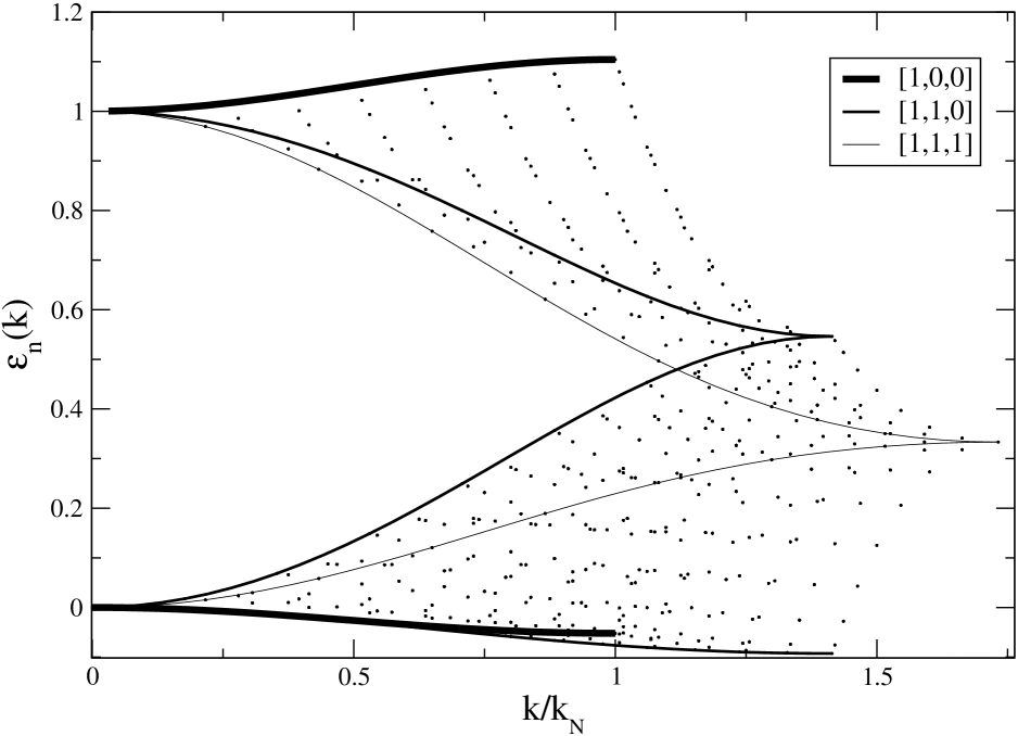
Figure 1: Eigenvalues $\epsilon_{n}({\bf k})$ for a sc lattice. The lines connect eigenvectors with ${\bf k}$ in the specific directions indicated. Note that the two acoustic branches are degenerate in the $[1,0,0]$ and $[1,1,1]$ directions.

In Fig. 1 are shown the eigenvalues of the dynamical matrix, for gravity, for a $16^{3}$ sc lattice, determined numerically by applying the linearization to a standard Ewald summation of the gravitational force (see e.g. ewald ). For convenience the eigenvalues have been normalized, with $\epsilon_{n}({\bf k})=-\frac{\omega_{n}^{2}({\bf k})}{4\pi G\rho_{0}}$, and they are plotted, as a function of the modulus $k\equiv|{\bf k}|$, normalized to the Nyquist frequency $k_{N}=\pi/l$, where $l$ is the lattice spacing. This diagonalisation can be performed rapidly even for the largest lattices used in current cosmological NBS, but the figure remains essentially unchanged except for an increase in the density of the eigenvalues. The lines in the figure connect the eigenvectors along some specific chosen directions, making the characteristic branch structure of the eigenvectors evident. It can be shown pines that ${\cal D}_{\mu\nu}({\bf k}\rightarrow 0)=-{\hat{k}}_{\mu}{\hat{k}}_{\nu}4\pi G\rho_{0}$ (where ${\bf\hat{k}}={\bf k}/k$), so the branch with eigenvalue tending to $-4\pi G\rho_{0}$ is longitudinal (in this limit). In the Coulomb lattice this is the optical branch, describing oscillations for $k\rightarrow 0$ with plasma frequency $\omega_{p}^{2}=4\pi e^{2}n_{0}/m$ (where $n_{0}$ is the electronic number density). There are then also two acoustic branches with eigenvalues tending to zero as $k\rightarrow 0$ and which become purely transverse in this limit. A striking feature of Fig.1 is that there are eigenvectors with $\epsilon_{n}({\bf k})<0$, which correspond to unstable modes for the Coulomb system, with solutions to Eq. (5) $U_{n}({\bf k},t)=\cosh(|\omega_{n}({\bf k})|t)$ and $V_{n}({\bf k},t)=(1/|\omega_{n}({\bf k})|)\sinh(|\omega_{n}({\bf k})|t)$ (taking $a=1$ and $t_{0}=0$). Thus the sc Coulomb lattice is unstable to perturbations, which is not an unexpected result: the ground state of this classical system is known to be the bcc lattice wc-ground state , and these unstable modes in the sc lattice correspond to instabilities towards such lower energy configurations. For the case of gravity, in a static universe, these modes are sinusoidally oscillating, while the modes $\epsilon_{n}({\bf k})>0$ describe the expected exponential instabilities. Note further that, since the Kohn sum rule can be written $\sum_{n}\epsilon_{n}({\bf k})=1$, the appearance of modes with $\epsilon_{n}({\bf k})>1$ is only possible when there are modes with $\epsilon_{n}({\bf k})<0$. Without calculation we can thus conclude that a bcc lattice will have only unstable modes in the case of gravity, and that $\epsilon_{n}({\bf k})\leq 1$. We will return to this point below.

The damping term coming from the expansion of the universe modifies these solutions to Eq. (5). For the case of an Einstein de Sitter (EdS, flat matter dominated) universe, for which $H^{2}(t)=\frac{8\pi G\rho_{0}}{3a^{3}}$ and thus $a=(t/t_{0})^{2/3}$, we find

$$U_{n}({\bf k},t) = \frac{\alpha_{n}^{+}({\bf k})(t/t_{0})^{\alpha_{n}^{-}({\bf k})}+\alpha_{n}^{-}({\bf k})(t/t_{0})^{-\alpha_{n}^{+}({\bf k})}}{\alpha_{n}^{+}({\bf k})+\alpha_{n}^{-}({\bf k})}$$

$$V_{n}({\bf k},t) = t_{0}\frac{(t/t_{0})^{\alpha_{n}^{-}({\bf k})}-(t/t_{0})^{-\alpha_{n}^{+}({\bf k})}}{\alpha_{n}^{+}({\bf k})+\alpha_{n}^{-}({\bf k})}$$ (6)

where $\alpha_{n}^{\pm}({\bf k})=\frac{1}{6}[\sqrt{1+24\epsilon_{n}({\bf k})}\pm 1]$. Thus for $\epsilon_{n}({\bf k})>0$ there are, as in the static case, both a growing and a decaying solution. For $\epsilon_{n}({\bf k})<0$ the solutions are all power-law decaying. For $\epsilon_{n}({\bf k})<-\frac{1}{24}$, there is a weak remnant of the static universe oscillating behaviour: $\alpha_{n}^{\pm}({\bf k})$ are then complex, and it is simple to show that the mode functions are a product of a power law $(t/t_{0})^{-\frac{1}{6}}$ and a sinusoidal oscillation periodic in the logarithm of the evolution time $\ln(t/t_{0})$.

Let us now consider the case that the initial fluctuations contain only modes s.t. $kl\ll 1$. We have then simply for each ${\bf k}$ the longitudinal mode ${\bf e}_{1}({\bf k})={\hat{\bf k}}$, with $\epsilon_{1}({\bf k})=1$, and two transverse modes with zero eigenvalues. Using the corresponding mode functions from Eq. (6), and Eq. (4), a simple calculation shows that

$${\bf u}({\bf R},t) ={\bf u}_{\perp}({\bf R},t_{0})+{\bf u}_{\parallel}({\bf R},t_{0})\left[\frac{3}{5}(\frac{t}{t_{0}})^{\frac{2}{3}}+\frac{2}{5}(\frac{t}{t_{0}})^{-1}\right]$$ (7)

$$+{\bf v}_{\parallel}({\bf R},t_{0})t_{0}\left[\frac{3}{5}(\frac{t}{t_{0}})^{\frac{2}{3}}-\frac{3}{5}(\frac{t}{t_{0}})^{-1}\right]$$

$$+{\bf v}_{\perp}({\bf R},t_{0})3t_{0}\left[1-(\frac{t}{t_{0}})^{-\frac{1}{3}}\right]$$

where we have decomposed the particle displacements and peculiar velocities (${\bf v}({\bf R},t)\equiv{\dot{\bf r}}_{i}-H{\bf r}_{i}=a{\bf{\dot{u}}}({\bf R},t)$) into an irrotational (curl-free) part ${\bf a}_{\parallel}({\bf R})=\frac{1}{N}\sum_{{\bf k}}({\bf a}({\bf R})\cdot{\bf{\hat{k}}}){\bf{\hat{k}}}\,e^{i{\bf k}.{\bf R}}$, and a rotational part ${\bf a}_{\perp}={\bf a}-{\bf a}_{\parallel}$. Using the definition of the peculiar gravitational acceleration ${\bf g}({\bf R},t)\equiv{\ddot{\bf r}}_{i}-\frac{\ddot{a}}{a}{\bf r}_{i}=a[{\bf{\ddot{u}}}+2H{\bf{\dot{u}}}]$, it is simple to show, using Eq. (2), that ${\bf g}({\bf R},t_{0})=4\pi G{\rho_{0}}{\bf u}_{\parallel}({\bf R},t_{0})=\frac{2}{3t_{0}^{2}}{\bf u}_{\parallel}({\bf R},t_{0})$. Using this expression in Eq. (7), the displacement of each particle with respect to its initial position (i.e. ${\bf u}({\bf R},t)-{\bf u}({\bf R},t_{0})$) can be written solely in terms of the initial gravitational field ${\bf g}({\bf R},t_{0})$ and the components of the initial peculiar velocity, ${\bf v}_{\perp}({\bf R},t_{0})$ and ${\bf v}_{\parallel}({\bf R},t_{0})$. It is then easy to verify that the solution in Eq. (7) corresponds exactly to that derived in buchert1992 , from a linearization of the Lagrangian equations for a self-gravitating fluid, for the displacements of fluid elements with respect to their Lagrangian coordinates . As discussed in buchert1992 there are several limits of this expression which correspond to the so called Zeldovich approximation (ZA), which assumes zeldovich-ZApaper a decomposition of ${\bf u}({\bf R},t)$ into a product of a function of time and a single vector field defined at ${\bf R}$. The most commonly used form of this approximation takes ${\bf u}_{\perp}({\bf R},t_{0})=0={\bf v}_{\perp}({\bf R},t)$ and ${\bf u}_{\parallel}({\bf R},t_{0})=\frac{3}{2}{\bf v}_{\parallel}({\bf R},t_{0})t_{0}$. This corresponds to setting the coefficients of all but the growing mode in Eq. (7) to zero i.e. it imposes directly the asymptotic behaviour of the general solution. We then have simply ${\bf u}({\bf R},t)=\frac{3}{2}{\bf g}({\bf R},t_{0})t_{0}^{2}(t/t_{0})^{\frac{2}{3}}$ which is precisely the solution used standardly in setting up initial conditions for cosmological NBS (e.g. nbs-standard-references ).

This result provides a direct analytical derivation explaining precisely the well documented success (see e.g. melott-ZA ) of the ZA in describing the evolution of cosmological NBS, in particular in “truncated” forms of the approximation in which initial short wavelength power is filtered truncatedZA . The eigenvectors and the spectrum of eigenvalues contain, however, much more than this fluid limit. The expression Eq. (4) gives an approximation to the full early time evolution of any perturbed lattice, treated as a full discrete $N$-body system. It therefore includes all modifications of the theoretical fluid evolution in its regime of validity, which extends up to the time when particles approach one another (i.e. up to close to “shell crossing”). We will report elsewhere detailed comparisons in numerical simulations of this approximation with the ZA and its improvements. In the rest of this letter we consider the quantification of the discreteness corrections to the pure fluid limit described by our approximation.

Assuming still an EdS universe, and that the initial perturbations are set up in the standard manner using the ZA, as described above, it follows directly from Eq. (4) that ${\tilde{u}}_{\mu}({\bf k},t)=\sum_{\nu}{\cal A}_{\mu\nu}({\bf k},t){\tilde{u}}_{\nu}({\bf k},t_{0})$, where ${\cal A}_{\mu\nu}({\bf k},t)=\sum_{n}[U_{n}(t)+\frac{2}{3t_{0}}V_{n}(t)]({\bf{\hat{e}}}_{n})_{\mu}({\bf{\hat{e}}}_{n})_{\nu}$ (the ${\bf k}$ dependences on the right hand side are implicit). The full linearised evolution is encoded in this matrix, which can be calculated straighforwardly for any given lattice once the eigenvalues and eigenvectors have been found. One can then determine directly e.g. the power spectrum (PS) of the displacement fields ${\cal S}_{\mu\nu}({\bf k},t)\equiv{{\tilde{u}}_{\mu}}({\bf k},t){{\tilde{u}}_{\nu}^{*}}({\bf k},t)$. Given ${\cal S}$ one can then calculate, by the method developed in gabrielli-pre-2004 , the PS of the density field for the full point distribution. For small displacements (compared to $l$) and neglecting the terms describing the discreteness of the lattice, it is a good approximation to use the continuity equation which gives $\tilde{\delta\rho}({\bf k},t)\approx-i{\bf k}\cdot{\tilde{\bf u}}({\bf k},t)$, where $\tilde{\delta\rho}({\bf k},t)$ is the FT of the density fluctuation field. It follows that $P({\bf k},t)\approx A_{P}^{2}({\bf k},t)P({\bf k},t_{0})$ where $A_{P}({\bf k},t)=\sum_{\mu,\nu}{\hat{k}}_{\mu}{\hat{k}}_{\nu}{\cal A}_{\mu\nu}({\bf k},t)$ and $P({\bf k},t)\propto|\tilde{\delta\rho}({\bf k},t)|^{2}$ is the PS of the density fluctuations. It is simple to verify that in the fluid limit discussed above ($kl\rightarrow 0$) one obtains, as expected, $A_{P}^{2}({\bf k},t)=a^{2}(t)$.

In Fig. 2 is shown this amplification factor $A_{P}^{2}({\bf k},t)$, divided by $a^{2}$. The scale factor chosen is $a=5$, a value at which typical NBS reach shell crossing. Deviations from unity are a direct measure of the modification of the theoretical evolution introduced by the discretisation. Note that $A_{P}^{2}({\bf k},a)$ is plotted as a function of $k$, each point corresponding to a different value of ${\bf k}$. The fact that the evolution depends on the orientation of the vector ${\bf k}$ is a manifestation of the breaking of rotational invariance by the lattice discretisation. The three different symbols for the points correspond to three different intervals of the cosine of the minimum angle $\theta$ between the vector ${\bf k}$ and one of the axes of the lattice. We thus see that the largest eigenvalues correspond to modes describing motion parallel to one of the axes of the lattice. For a $N^{3}$ lattice and $N$ even, for instance, the largest eigenvalue, with a growth law $\propto a^{1.06}$, is a longitudinal mode with $k=k_{N}$ and ${\bf k}$ parallel to the axes of the lattice, which describes the motion of pairs of adjacent infinite planes towards one another. Also shown in the figure is an average of $A_{P}^{2}({\bf k},a)$ over 25 bins of equal width in $k$, both for the $16^{3}$ lattice from which the points have been calculated, and for a larger $64^{3}$ lattice.

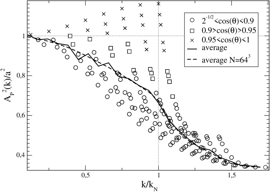
Figure 2: Amplification function $A_{P}^{2}({\bf k},t)$ for the power spectrum, divided by the fluid limit amplification ($a^{2}$), at $a=5$, for a sc lattice. See text for details.

We thus see that there are qualitatively two kinds of effects introduced by the discretisation: (i) an average slowing down of the growth of the modes relative to the theoretical fluid evolution, and (ii) a pronounced anistropy in $k$-space. There are notably a small fraction of modes (approximately 2.5 %) with growth exponents larger than in linear fluid theory (which, for sufficiently large $a$, will always dominate the evolution). We can conclude, however, as foreshadowed in the discussion above, that this evidently undesirable feature of the sc lattice discretisation can be circumvented by employing a bcc lattice. The known stability of this configuration of the Coulomb lattice wc-ground state implies that the fluid exponent is in this case an upper bound for all modes (and that there are no oscillating modes for the case of gravity). Further the bcc crystal is more isotropic (and indeed more compact torquato ) than the sc lattice, and thus we would expect the effects of breaking of isotropy to be less pronounced. The average slowing down of the growth of the modes, by an amount which depends on the time and the dimensionless product $kl$ (at $a=5$, as seen in Fig. 2, a 10% effect at half the Nyquist frequency), on the other hand, would be expected to be a common feature of any discretisation (e.g. using “glassy” configurations white-leshouches , or the discretisation developed in mj-dl-bm-initial-conditions ).

This analysis does not, of course, allow one to conclude fully about the role of discreteness effects in the longer time evolution of such simulations. It should provide, however, a first step to the quantitative understanding of these effects. One important conclusion which we can draw is the following: for a given physical wavelength, the discrepancy between the fluid and full evolution grows, up to shell crossing, with time. Thus, for a given physical scale, discreteness effects increase when the starting time of the simulation is decreased. For the particular case of the sc lattice it is clear that artificial collapses of infinite planes along the axes of the lattice, which grow more rapidly than even long-wavelength fluid modes, will be increasingly priveleged as earlier starting times are taken. This implies that at least one of the conditions for keeping discreteness effects under control in an NBS will be a constraint on the initial time (i.e. that the starting red-shift be greater than some value, given the discretisation scale). We note that the initial red-shift is not a parameter considered in discussions of discreteness effects in NBS in the literature (e.g. discreteness-references ; discreteness-hamana ).

We can extend our treatment easily to incorporate a smoothing of the gravitational force up to a scale $\epsilon$. Here we have taken pure gravity (i.e $\epsilon=0$) as in most cosmological NBS $\epsilon\ll l$, which gives negligible modification of our results. Just as in the analogous condensed matter system, the method can also be extended to higher order. It would be interesting in particular to map at higher order this description of the discrete system onto the corresponding order of fluid Lagrangian theory, which has been explored extensively in the cosmological literature (see e.g. higher-order-lagragian stuff , and references therein). Further it should be possible to use the approach presented here to understand better the nature of existing approximations which go beyond the simple fluid limit, for example those involving pressure terms associated to velocity dispersion (see e.g. higher-order-lagragian stuff ; buchert-dominguez and references therein).

References

- (1) G. Efstathiou et al, Astrophys. J. Supp. 57, 241 (1985).
- (2) D. Pines, Elementary Excitations in Solids, Benjamin (1963).
- (3) Ya. Zeldovich, Astron. Astrophys. 5, 84 (1970).
- (4) A. Melott and S. Shandarin, Ap. J. 410, 469 (1993); A. Melott et al., Ap. J. Lett. 479, 79 (1996); R. Splinter et al., Ap. J. 497, 38 (1998).
- (5) T. Baertschiger et al., Ap. J. Lett. 581, L63-L66 (2002).
- (6) T. Hamana at al.,, Ap. J. 568, 455 (2002).
- (7) L. Hernquist et al., Astrophys.J. Supp. 75, 231 (1991).
- (8) R.R. Sari et al., J. Phys. A : Math. Gen. 9 1539 (1976).
- (9) T. Buchert, Mon. Not. R. Astron. Soc. 254, 729 (1992).
- (10) A. Melott, Ap. J. 426, L19 (1994).
- (11) P. Coles et al., Mon. Not. R. Astron. Soc. 260, 765 (1993).
- (12) A. Gabrielli, Phys. Rev. E 70, 066131 (2004).
- (13) S. Torquato, and F. H. Stillinger, Phys. Rev. E 68, 041113 (2003).
- (14) S.D.M. White, astro-ph/9410043.
- (15) M. Joyce, D. Levesque and B. Marcos, astro-ph/0411607.
- (16) T. Tatekawa, astro-ph/0412025.
- (17) T. Buchert and A. Dominguez, astro-ph/0502318.