On the Dayside Thermal Emission of Hot Jupiters

Abstract

We discuss atmosphere models of HD209458b in light of the recent day-side flux measurement of HD209458b’s secondary eclipse by Spitzer-MIPS at 24 $\mu$m. In addition, we present a revised secondary eclipse IRTF upper limit at 2.2 $\mu$m which places a stringent constraint on the adjacent H₂O absorption band depths. These two measurements are complementary because they are both shaped by H₂O absorption and because the former is on the Wien tail of the planet’s thermal emission spectrum and the latter is near the thermal emission peak. A wide range of models fit the observational data, confirming our basic understanding of hot Jupiter atmospheric physics. Although a range of models are viable, some models at the hot and cold end of the plausible temperature range can be ruled out. One class of previously unconsidered hot Jupiter atmospheric models that fit the data are those with C/O $\gtrsim$1 (as Jupiter may have), which have a significant paucity of H₂O compared to solar abundance models with C/O = 0.5. The models indicate that HD209458b is in a situation intermediate between pure in situ reradiation and very efficient redistribution of heat; one which will require a careful treatment of atmospheric circulation. We discuss how future wavelength-dependent and phase-dependent observations will further constrain the atmospheric circulation regime. In the shorter term, additional planned measurements for HD209458b, especially Spitzer IRAC photometry, should lift many of the model degeneracies. Multiwavelength IR observations constrain the atmospheric structure and circulation properties of hot Jupiters and thus open a new chapter in quantitative extrasolar planetology.

1 Introduction

The star HD209458 is the brightest known ($V=7.5$) to host a short-period giant planet which transits the face of the star (Charbonneau et al., 2000; Henry et al., 2000). Recently Deming et al. (2005b) detected the secondary eclipse of the planet by the star in this system, at a wavelength of 24$\mu$m using the MIPS instrument on the Spitzer Space Telescope. The measured flux decrement during secondary eclipse provides a direct measurement of the planetary day side thermal emission. Together with the recent Spitzer IRAC secondary eclipse detection of TrES-1 (Charbonneau et al., 2005), this marks the first measurement of the thermal emission from a known extrasolar planet.

In this paper we examine what constraints can be placed on the planetary properties by this historic measurement. While our principal constraint is the measured 24 micron flux ($F_{24\mu{\rm m}}$) there are several additional observational data points useful for the study of the HD209458b atmosphere. The most relevant additional constraint for the planetary day side flux is an upper limit on the H₂O absorption band depths on either side of the 2.2 $\mu$m continuum flux peak ($\Delta F_{2.2\mu{\rm m}}$), reported by Richardson et al. (2003). Two data points from transmission spectra of the lower atmosphere—which probe the planetary limb—are relevant: the Na resonance doublet detection at 0.584 $\mu$m (Charbonneau et al., 2002) and an upper limit on CO at 2 $\mu$m (Deming et al., 2005a). With these data, we can begin to constrain atmosphere models of the extrasolar planet HD209458b.

The new Spitzer data is consistent with a circular orbit for HD209458b, based on the equal time spacing between primary and secondary eclipses (Deming et al., 2005b). In addition, the latest radial velocity determination of the eccentricity is essentially zero: $e=0.013\pm 0.009$ (Laughlin et al., 2005). With a circular orbit, the anomalously large radius of HD209458b is not explained by an interacting companion (Bodenheimer et al., 2003; Deming et al., 2005b). While atmospheric processes have also been hypothesized to play a role in the radius evolution of HD209458b (Guillot & Showman, 2002), to first-order, the atmospheric circulation regime on the $\sim$ 3-day period hot Jupiters with radii closer to Jupiter’s is not expected to differ much (Menou et al., 2003). The $F_{24\mu{\rm m}}$ also indicates that the planet HD209458b is in synchronous rotation with its orbit, presenting the same face to the star at all times. Because the timescale for synchronization is much smaller than the timescale for orbital circularization (Goldreich & Soter, 1966), the tidally-locked assumption is likely valid. The notion of a permanent day side has important consequences for model atmospheres and data interpretation because it means only one side of the planet is being heated by the star.

We begin by describing the HD209458b $F_{24\mu{\rm m}}$ measurement and $\Delta F_{2.2\mu{\rm m}}$ upper limit in §2. In §3 we describe the radiative transfer models and their uncertainties. In §4 we present a comparison of the models with the HD209458b data as well as a discussion of the relation between the observations of TrES-1 and HD209458b. In §5 we consider the broader implications and near-term prospects for both theory (§5.1) and observation (§5.2). We conclude in §6 by describing how specific upcoming observations of HD209458b will enable a more definitive atmospheric characterization.

2 HD209458b Secondary Eclipse Data

In this paper we focus on the thermal emission data. Both $F_{24\mu{\rm m}}$ and $\Delta F_{2.2\mu{\rm m}}$ are secondary eclipse measurements which probe the planetary day side thermal emission.

2.1 The Spitzer 24$\mu$m Flux

The HD209458b secondary eclipse measured by Spitzer yields a planet/star flux ratio $F_{24\mu{\rm m}}/F_{*}=0.00260\pm 0.00046$, a 5.6$\sigma$ result. During secondary eclipse the planet is obscured and only starlight is present. The resulting flux decrement yields the ratio of planet to stellar flux. Multiplying this by the measured stellar flux at this wavelength ($21.17\pm 0.11$ mJy), the planetary flux is thus measured to be $F_{24\mu{\rm m}}=55\pm 10~{}\mu$Jy.

2.2 The IRTF 2.2 $\mu$m Constraint

Hot Jupiter atmosphere models generically predict a peak in the continuum near 2.2 $\mu$m due to the combined influence of water and CO absorption (with CO a relatively weak component at 2.3 $\mu$m). Richardson et al. (2003) used the method of “occultation spectroscopy” to search for this signature during the HD209458b secondary eclipse using the NASA Infrared Telescope Facility (IRTF) SpeX (Rayner et al., 2003) spectral data from 1.9 to 4.2 microns at a spectral resolution of $\Delta\lambda/\lambda=1500$. We have revisited the data to improve the upper limit.

The data do not provide an absolute upper limit to the 2.2$\mu$m flux itself. The differential nature of the observations means that only a relative measurement among the data points in the specified spectral range is possible. We therefore calculate the upper limit to the flux difference, or band depth, at the location in the spectrum where an absorption band is expected. Note that the data points are expressed in terms of the star-planet flux ratio. We use three data bins: a central bin where the flux peak is predicted to reside (2.09–2.31$\mu$m), and one bin on either side of the flux peak bin where an absorption band trough should appear (1.955–2.09$\mu$m and 2.31–2.52$\mu$m). The difference between the flux peak bin and the absorption trough bins are $2.02\times 10^{-5}\pm 1.25\times 10^{-4}$ and $9.78\times 10^{-6}\pm 1.52\times 10^{-4}$ respectively. We average these two values to obtain an average band depth of $1.5\times 10^{-5}\pm 9.8\times 10^{-5}$. Since the result is essentially zero, we take the error on the mean $\sim 1\times 10^{-4}$ to be the upper limit on the band depth on either side of the 2.2 $\mu$m flux peak at the $1\sigma$ level.

We convert this contrast ratio limit into a flux limit of $\Delta F_{2.2\mu{\rm m}}=200\mu$Jy (see Figure 1), using a Kurucz model atmosphere for the star (Kurucz, 1992) and the HD209458b planet-star area ratio (using $R_{p}=1.347\pm 0.060R_{J}$ and $R_{*}=1.146\pm 0.050R_{\odot}$ from Brown et al., 2001). To summarize, the $\Delta F_{2.2\mu{\rm m}}$ constraint means that the band depths from the continuum peak to the absorption trough must be $<200\mu$Jy. This proves to be a useful constraint and is discussed further in relation to model atmospheres in §3.

3 HD209458b Atmosphere Models

Model atmosphere computations are required for an interpretation of spectral data because the planetary fluxes at different wavelengths are shaped by a variety of physical processes. Measurements of the flux level at only one or two wavelengths can be very misleading if not interpreted in the appropriate model context.

3.1 Background and Caveats

Model spectra were computed with a 1D plane parallel radiative transfer code. This code solves three equations: the equation of radiative transfer, the equation of radiative equilibrium, and hydrostatic equilibrium to derive three unknowns: temperature (as a function of altitude), pressure (as a function of altitude) and the radiation field (as a function of altitude and wavelength). The boundary conditions are the stellar radiation at the top of the atmosphere, and the interior entropy at the bottom of the atmosphere. The model outputs are temperature, pressure, and radiation field (from which the emergent flux can be computed). From the wavelength-integrated thermal emission flux ($F$), $T_{eq}$ can be calculated by $(F/\sigma_{R})^{1/4}$ where $\sigma_{R}$ is the radiation constant, and the geometric albedo can be computed by ratioing the visible-wavelength emergent flux to the incident stellar flux.

Although the physics of this 1D model is straightforward, it is necessary to choose several input parameters, which thus constitute uncertainties with various levels of impact. The interior entropy is unknown, although it can be estimated from evolutionary models. Opacities govern the absorption and reemission of radiation and so drive the entire radiative transfer problem, determining the vertical temperature-pressure profile and the planetary flux. The choices of metallicity, which atomic and molecular species to include, whether to include only equilibrium or non-equilibrium chemistry as well, all affect the opacities and are thus input parameters. Clouds are the most serious uncertainty in terms of opacities. They form at a the saturation vapor pressure and (for solar system planets) can extend 1 to 2 pressure scale heights above this “cloud base”. Dozens of high temperature condensates could potentially exist; only a few are suspected to have a significant magnitude of opacity. The condensate opacity is controlled by particle size distribution and index of refraction, as well as particle shape. Although cloud models have been used by some researchers to compute the particle size distribution and cloud vertical extent for spherical particles (Ackerman & Marley, 2001; Cooper et al., 2003), they still have as a free parameter the type of condensate and the amount of condensed material in the cloud (e.g., by specifying the efficiency of sedimentation). All extrasolar planet atmospheres models in the literature consider horizontally homogeneous clouds (i.e., covering the entire planet).

Finally, for 1D models we must also make an assumption of how the incident stellar radiation is redistributed across the surface of the planet. We use the parameter $f$ (described in §4.1) as the proxy for atmospheric circulation: $f=1$ if the absorbed stellar radiation is redistributed evenly throughout the planet’s atmosphere (e.g., due to strong winds rapidly redistributing the heat) and $f=2$ if only the heated day side reradiates the energy (for the latter $T_{eq}$ is for the day side only). The implementation in the models is achieved by multiplying the incoming stellar radiation by a factor of $f/4$.

3.2 Model Choices

In terms of choices for the models presented here, we use: a Kurucz model atmosphere for the stellar radiation (Kurucz, 1992); solar abundances (HD209458A is close to solar metallicity with [Fe/H] = 0.04 (Gonzalez et al., 2001); and line opacities of H₂O, CH₄, CO, Na, K, and collision-induced absorption opacities of H₂-H₂ (Borysow et al., 2001) and H₂-He (Jørgensen et al., 2000). We adopt a planetary interior energy flux corresponding to an effective temperature $T_{\rm eff}=500$ K. A Gibbs Free energy minimization code was used to compute chemical equilibrium (Seager, 1999). H₂ Rayleigh scattering and scattering and absorption by MgSiO₃ and Fe vertically and horizontally uniform and homogenous clouds are included with a specified particle size distribution (a log normal distribution with particle radius of 2 $\mu$m and $\sigma=0.05$) and vertical extent (two pressure scale heights above the cloud base) are also included. Note that for computational efficiency we use a separate, higher spectral resolution, radiative transfer code with the same input assumptions to compute the final emergent spectra based on the T/P profiles. A more detailed description of the code and opacity sources can be found in Seager (1999) and Seager et al. (2000). (See Barman et al., 2001; Sudarsky et al., 2003; Burrows et al., 2005; Fortney et al., 2005, for choices made by other modelers).

With all of the above uncertainties there are many choices that lead to a wide range of models for a given planet. Rather than an exhaustive search of the model parameter space, we consider three models (Figure 1) which span a range of reasonable possibilities, to interpret the HD209458b $F_{24\mu{\rm m}}$ and $\Delta F_{2.2\mu{\rm m}}$ data. Model 1 is possibly the simplest case one can consider; an $f=2$, cloud-free model with solar abundances. The second case, model 2, is a similarly simple model, but now with $f=1$, so that some energy is redistributed to the night side. Model 3 illustrates the effects of thick clouds; it is an $f=1$ model with thick, high clouds given by the parameters described above.

4 Data Interpretation

4.1 Planetary Equilibrium Temperature

The planetary equilibrium effective temperature $T_{eq}$ is a fundamental parameter of the planetary atmosphere and is useful as a proxy for the global temperature of a planet atmosphere. To first order $T_{eq}$ tells us how much radiation is being absorbed by the dayside of the planet. In this subsection we relate the measured $F_{24\mu{\rm m}}$ to $T_{eq}$.

The measured flux $F_{24\mu{\rm m}}=55\pm 10\mu$Jy can be converted into a 24$\mu$m brightness temperature $T_{24\mu{\rm m}}=1130\pm 150$ K (Deming et al., 2005b). The brightness temperature is the temperature of a blackbody emitting the flux equivalent at a specific wavelength and is not necessarily an accurate representation of the planet’s equilibrium effective temperature $T_{eq}$. Only if the planet radiates as a blackbody is $T_{eq}$=$T_{24\mu{\rm m}}$.

The spectrum of a hot Jupiter, however, is expected to be very different from a blackbody due primarily to strong H₂O absorption throughout near-IR and mid-IR wavelengths. In particular, in the mid-IR (which is the spectral region probed by MIPS) H₂O has strong continuous absorption such that there is no true planetary continuum expected from models at the MIPS wavelength bands, even though the relatively flat spectrum makes it appear so. In other words, the H₂O vapor absorption in the 24 $\mu$m region substantially depresses the planetary flux. This implies that if H₂O vapor absorption is present, the true $T_{eq}>1130$ K. Figure 1 shows the theoretical spectrum of our three HD209458b example models; each of these models match $F_{24\mu{\rm m}}$ even though their $T_{eq}$ (1700 K, 1420 K, and 1450 K respectively) are all hotter than $T_{24\mu{\rm m}}$. We also show the blackbody spectrum for these temperatures to demonstrate how significantly $F_{24\mu{\rm m}}$ is suppressed by H₂O absorption in these models (a flux depression equivalent to a decrease of $\sim$ 300–600 K in $T_{24\mu{\rm m}}$).

The true equilibrium temperature is regulated by several competing physical effects—the amount of irradiation received from the host star, the fraction that is simply reflected rather than absorbed (governed by the Bond albedo $A_{B}$), and the amount of energy circulated away from the hotter regions by hydrodynamic processes in the atmosphere. Considering energy balance between the absorbed and reemitted flux for a planet with zero eccentricity and ignoring any (likely much smaller) contribution from the planetary interior,

$$T_{eq}=T_{*}\left(\frac{R_{*}}{2a}\right)^{1/2}\left[f(1-A_{B})\right]^{1/4},$$ (1)

where $R_{*}$ is the stellar radius, $T_{*}$ is the stellar effective temperature, $a$ the semi-major axis, and $A_{B}$ the Bond albedo. Here $f$ is the proxy for atmospheric circulation, derived by considering whether the incident stellar radiation is reemitted into $4\pi$ steradians ($f=1$) if the absorbed stellar radiation is redistributed evenly throughout the planet’s atmosphere (e.g., due to strong winds rapidly redistributing the heat) or reemitted into $2\pi$ steradians ($f=2$) if only the heated day side reradiates the energy (for the latter $T_{eq}$ is for the day side only). Figure 2a shows $T_{eq}$ for the HD209458 parameters ($T_{*}=6000$ K, $R_{*}=1.18R_{\odot}$, and $a=0.046$ AU; Mazeh et al., 2000; Cody & Sasselov, 2002).

An equilibrium temperature $T_{eq}=1700$ K is at the hot end of the range for the HD209458 system parameters, as shown in Figure 2. If our model 1 with $T_{eq}=1700$ K were the unique, correct planetary model, this hot $T_{eq}$ would have significant implications: it is only plausible with both a low $A_{B}$ and no heat redistribution (i.e., $f=2$). At the low end of the plausible temperature range, $T_{eq}=1130$ K is unlikely. A $T_{eq}=1130$ K model would require that HD209458b has a very high Bond albedo ($>0.65$), and would probably require $f=1$ because $A_{B}>0.8$ is difficult to attain. Most of the solar system planets have $A_{B}<0.35$, with the exceptions of Venus ($A_{B}=0.75$) and Pluto ($A_{B}=0.4$) (de Pater & Lissauer, 2001).

4.2 Constraints on Models

Model 1 (solar metallicity, no clouds, no energy redistribution) is characterized by strong near-IR H₂O vapor absorption bands. The H₂O absorption also causes a strong depression of $F_{24\mu{\rm m}}$. With the strong alkali metal absorption dominating H₂ Rayleigh scattering at visible wavelengths, this model has a low albedo (geometric albedo = 0.15) and hence high $T_{eq}=1700$ K.

The Na detection and CO upper limit transmission spectroscopy are both too weak to match a solar abundance cloud-free chemical equilibrium model (Charbonneau et al., 2002; Deming et al., 2005b) and therefore in general provide a useful model constraint. In this cloudless case the Na could be transported to the night side and converted to Na₂S at the lower temperatures (Guillot & Showman, 2002; Iro et al., 2005); similarly CO would be converted to CH₄ on the night side, thus also potentially satisfying the limits from transmission spectroscopy. It is important to keep in mind that the transmission spectroscopy probes the planetary limb; with $f=2$, the day and night side are assumed to be different temperatures and so the planetary limb could have different conditions from those computed on the day side, for example a high cloud at the limb due to the falling temperatures away from the substellar point. This high cloud would also satisfy the Na and CO limits from transmission spectroscopy.

We use this $T_{eq}=1700$ K model as an example of a model that is ruled out by the data. Although this model satisfies $F_{24\mu{\rm m}}$ and can satisfy the transmission spectra data, it is ruled out (at the $5\sigma$ level) by the $\Delta F_{2.2\mu{\rm m}}$ data. The strong water vapor absorption bands adjacent to 2.2$\mu$m are in conflict with the $\Delta F_{2.2\mu{\rm m}}$ limit. The $\Delta F_{2.2\mu{\rm m}}$ constraint means that the band depths from the continnuum peak to the absorption trough must be $<200\mu$Jy, whereas in this model the band depths are $\sim 1000\mu$Jy. We used this simple model in Deming et al. (2005b) primarily to illustrate that $T_{eq}$ does not have to equal $T_{24\mu{\rm m}}$. The fact that model 1 is ruled out by our revised 2.2 $\mu$m upper limit shows that $\Delta F_{2.2\mu{\rm m}}$ is a useful constraint on models.

Model 2 (in which energy is now redistributed to the night side) has a lower computed $T_{eq}=1420$ K. While this model fits $F_{24\mu{\rm m}}$, it only fits the $\Delta F_{2.2\mu{\rm m}}$ constraint at the $3\sigma$ level due to the strong H₂O absorption features. In the context of this $f=1$ cloud-free, solar abundance model we note that the atmospheric circulation could allow for substantially varying temperatures at different horizontal locations (e.g., Showman & Guillot, 2002; Cho et al., 2003; Cooper & Showman, 2005) and so more detailed models may show partial cloud cover and lower Na abundances from molecular condensation (which may also better fit the weak Na and CO transmission spectra).

In Model 3 we allow for formation of thick, absorptive clouds and so, in contrast to models 1 and 2, it has very weak absorption band features with a computed $T_{eq}=1450$ K. The absorption and remission and scattering from largely grey cloud particles causes the absorption bands, including the continuous H₂O absorption at 24 microns, to be much shallower than in a cloud-free model. The cloud bases are computed to be at 5 and 10 millibar for MgSiO₃ and Fe respectively, with the cloud tops two pressure scale heights above at 0.8 and 1.3 millibar; this is consistent with both the lower-than-expected Na and CO transmission spectra. As seen from Figure 1 this model fits both the $\Delta F_{2.2\mu{\rm m}}$ and $F_{24\mu{\rm m}}$ data. We emphasize that the amount of condensates and their opacity strength (controlled by particle type and size distribution for spherical particles) hugely affects the overall spectrum; the condensate opacity is competing with the H₂O opacity to determine the water absorption band strengths. Different choices for the particle type, fraction of species condensed, cloud vertical scale height, and particle size distribution will all affect the overall opacity. Just one example is that larger particle sizes are likely to be more reflective and would not weaken the absorption bands nearly as much as absorptive particles.

4.3 Consequences of Model Constraints

Based on our investigation of models 1 through 3, we can draw some general conclusions. We showed above that the $T_{eq}=1700$ K model, under our adopted input assumptions (described in §4), is ruled out based on the $\Delta F_{2.2\mu{\rm m}}$ absorption band depth constraint. Other hot models are also ruled out by the data. First, a truly isothermal cloud-free atmosphere would satisfy the $\Delta F_{2.2\mu{\rm m}}$ because a vertically isothermal LTE atmosphere does not have any spectral features—i.e., it is a blackbody spectrum. However, such an isothermal $T_{eq}=1700$ K model is ruled out by the $F_{24\mu{\rm m}}$ data even considering the $3\sigma$ error on $T_{24\mu{\rm m}}$ which permits a value as high as 1580 K. Second, most hot models in between the isothermal atmosphere and the strong vertical temperature gradient atmosphere are likely ruled out; as the vertical temperature gradient gets shallower and satisfies $\Delta F_{2.2\mu{\rm m}}$ with a weaker absorption band, the 24 $\mu$m model flux gets higher and away from the measured $F_{24\mu{\rm m}}$. Third, a hot atmosphere with clouds that are highly absorptive (low $A_{B}$), such as Fe clouds, could also result in a blackbody spectrum (even without an isothermal atmosphere)—again a hot blackbody or near blackbody spectrum is ruled out because $T_{24\mu{\rm m}}=1130$ K is lower than resulting values of $T_{eq}$.

A second category of models that are difficult to fit are those with $T_{eq}$ at the cold end of the plausible range (equation (1) and Figure 2). As described above, for HD209458b to have a $T_{eq}$ near 1130K, a very high $A_{B}>0.65$ is required. Such a high $A_{B}$ could be possible only from a narrow range of cloud parameters and is not attainable in the absence of clouds—i.e., due to Rayleigh scattering alone.

Both of our $f=1$ and $f=2$ cloud-free models have a strong H₂O absorption band on either side of the 2.2 $\mu$m flux peak that do not fit the $\Delta F_{2.2\mu{\rm m}}$ constraint at the $1\sigma$ level. What could cause weaker H₂O absorption features to fit $\Delta F_{2.2\mu{\rm m}}$? Absorption and remission by cloud particles weaken the 2.2 $\mu$m absorption feature and are hence consistent with the data. A more isothermal atmosphere would also have weaker absorption features (see above). Decreasing the water vapor abundance could also serve to weaken the water vapor absorption features adjacent to 2.2 $\mu$m. This situation is hard to physically realize in a solar abundance atmosphere. Photodissociation from stellar UV radiation affects water only in the upper atmosphere, close to the microbar pressure level (Liang et al., 2003) where the low H₂O abundance would have little effect on the overall planetary spectrum.

4.4 Low H₂O Abundance in the C/O $\gtrsim$ 1 Regime

A possible scenario with a very low abundance of water vapor, that would satisfy $\Delta F_{2.2\mu{\rm m}}$, is one with atmospheric abundances of the carbon-to-oxygen ratio C/O $\gtrsim 1$. This is in contrast to the solar C/O ratio used in all extrasolar planet models published so far (0.5 or 0.42, Allende Prieto et al., 2002; Anders & Grevesse, 1989, respectively). In addition to being metal-rich overall, Jupiter is likely enriched in C with C/O = 1.8 (Lodders, 2004). In addition, Saturn has less oxygen enrichment than other heavy elements, including carbon (Visscher & Fegley, 2004). The enhanced metallicity on Jupiter and the other solar system planets is thought to come from post-formation planetesimal accretion and may well be applicable to hot Jupiters; enriched C compared to O over solar abundances would require pollution from carbon-rich planetesimals.

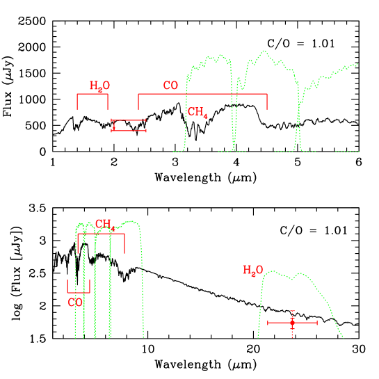
Figure 3: Thermal emission spectrum for HD209458b with C/O = 1.01 (and other elements in solar abundance). This chemical regime results in much reduced water abundance and increased CH₄ opacity compared to the solar abundance spectra shown in Figure 1. The $\Delta F_{2.2\mu{\rm m}}$ constraint and $F_{24\mu{\rm m}}$ measurement are shown, as are the IRAC and MIPS bandpasses (dotted lines).

A high C/O ratio $\gtrsim 1$ can have a large effect on the spectral signatures of hot planetary atmospheres (see Figure 3 and Figure 1 in Kuchner & Seager, 2005, Seager & Kuchner, in preparation). This is because at high temperatures the dominant carbon-bearing molecule is CO, and in equilibrium formation of CO is chemically favored instead of H₂O. In an extreme case, then, with all of the O tied up in CO, there will be no H₂O vapor present. In reality, depending on the temperature-pressure profile, there will be a small amount of water vapor present, but a few to $>$ eight orders of magnitude below the CO number density. This extreme paucity of H₂O is significant, because the hot Jupiter spectra are normally predominantly shaped by H₂O absorption bands. In the C/O $>$ 1 case the planetary spectrum will instead be dominated by CO absorption and by CH₄ absorption (which forms at higher temperatures than for C/O $<1$). (Note that for 0.5 $<$ C/O $<$1, the water vapor will decrease much less significantly, by a factor of a few to 100 respectively. See Fortney et al. (2005) for a discussion of the effects of C/O = 0.7.) In contrast to the hot Jupiter case, a C/O ratio $\gtrsim 1$ has a much less significant effect on the spectral signatures of planetary atmospheres cooler than the hot Jupiters (below $T_{eq}\sim$ 1000 K). In this case CH₄ is the dominant carbon-bearing molecule regardless of the C/O value; whatever O is present is free to form H₂O.

Any hot Jupiters with C/O $\gtrsim$ 1 should have a very low amount of water vapor, more so for those at the hot $T_{eq}$ range and those with hot upper atmospheres. Figure 3 shows an estimated thermal emission spectrum (using a scaled model 1 T/P profile to reproduce a $T_{eq}=1600$ K) with (condensate-free) chemical equilibrium computed for a value of C/O = 1.01. More careful modeling is needed to explore the consequences of a carbon-enriched hot Jupiter atmosphere, particularly for condensate formation which is affected by the O abundance. For C/O $>1$ graphite and SiC clouds can form which are not present in C/O $<1$ models.

4.5 HD209458b and TReS-1 Comparison

We now turn briefly to a discussion of the thermal emission detected from TrES-1, and how it relates to HD209458b day side thermal emission. The secondary eclipse detection of TrES-1 (Alonso et al., 2004) by Charbonneau et al. (2005) at Spitzer IRAC bands (4.5 and 8 $\mu$m) was reported at the same time as the HD209458b secondary eclipse detection. A planetary brightness temperature was reported at each bandpass: $T_{4.5\mu{\rm m}}=1010\pm 60$ K and $T_{8\mu{\rm m}}=1230\pm 110$ K, with an average $T_{\rm TrES-1}=1060\pm 60$ K. In this section we consider the TrES-1 data as it relates to HD209458b.

As for HD209458b, $T_{\rm TrES-1}$ does not constrain $A_{B}$ due to the unknown atmospheric redistribution of absorbed stellar radiation ($f$ in equation $\left(1\right)$; c.f. Charbonneau et al., 2005). If $T_{\rm TrES-1}=T_{eq}=1060$ K (shown in Figure 2b for the TrES-1 parameters $R_{*}=0.85R_{\odot}$, $T_{*}=5250$ K, $a=0.039$ AU; Alonso et al., 2004), then $0.3<A_{B}<0.7$, a large range. Using the same arguments as for HD209458b (non-blackbody-nature of the spectrum due primarily to H₂O absorption) the $T_{eq}$ is likely to be hotter than 1100K. A very interesting consequence of TrES-1 stellar temperature and planet semi-major axis is that if $T_{eq}>1200K$ an $f=1$ model is ruled out, otherwise we would have the unphysical situation $A_{B}<0$.

We emphasize that HD209458b and TrES-1 are likely to be different planets in terms of their atmospheric structure. We caution that the similar measured brightness temperatures of TrES-1 and HD209458b are misleading; they are at different wavelengths and probably probe different atmospheric altitudes/temperatures. Furthermore, TrES-1 and HD209458b are theoretically likely to have different $T_{eq}$ due to the former’s intrinsically fainter parent star (K0V ($T_{\rm eff}=5250$ K) vs. G0V ($T_{\rm eff}=6000$ K) respectively; see Figure 2). This temperature difference could have important consequences in terms of cloud altitude and the CO/CH₄ abundance ratio. A cold model for TrES-1 would have more CH₄ in the atmosphere than the hotter HD209458b models, for the same abundances. The two planets are also different in their radii (for HD209458b $R_{P}=1.347\pm 0.060R_{J}$ (Brown et al., 2001) and for TrES-1 $R_{P}=1.08_{-0.04}^{+0.18}R_{J}$ (Alonso et al., 2004)).

Although the two planets are different, it is still instructive to compare the TrES-1 data to the HD209458b models (Figure 1), since the solar abundance models have the same generic H₂O and CO absorption features at 4.5 and 8 $\mu$m. It is certainly puzzling that the $8\mu$m flux is $\gtrsim$ the $4.5\mu$m flux, because one generally expects more thermal emission at shorter wavelengths (see Figure 1). The TrES-1 data constrain the relative flux ratios of a shallow H₂O band at $8\mu$m and a deeper H₂O + CO band at 4.5 microns. For most model fluxes that match the $8\mu$m band the model fluxes are too high in the $4.5\mu$m band (Charbonneau et al., 2005) but only marginally so considering the $3\sigma$ errors on the data.

One solution to the IRAC $8\mu$m and $4.5\mu$m data discrepancy (Charbonneau et al., 2005) is a missing source of opacity at 4.4$\mu$m to cause a deeper absorption band. This discrepancy is at face value opposite to the requirement of weak H₂O bands for HD209458b from $\Delta F_{2.2\mu{\rm m}}$. Additional H₂O opacity would not likely solve the IRAC measurement discrepancy, because H₂O is present in both observed IRAC bands. An increased CO abundance without an increased H₂O abundance could potentially solve the problem because CO absorbs in the 4.4 $\mu$m band and not the 8 $\mu$m. A higher CO number density and lower H₂O number density could be realized with a higher C/O ratio than solar (but not necessarily C/O $>$1), as long as not too much CH₄ is present (which also absorbs in the 8$\micron$ IRAC band and whose number density grows as C/O increases) (Seager & Kuchner, in preparation). See Fortney et al. (2005) for a discussion of metallicity and varying C/O ratios for TReS-1 models. A second solution to fit the nearly equal fluxes in the IRAC $8\mu$m and $4.5\mu$m bands is a close-to-vertically isothermal model with weaker absorption bands. Such a model would have to be a cool model to fit the data, as illustrated by the blackbody fit in Figure 1 and in Charbonneau et al. (2005). We note that a cooler model fit indicates that efficient redistribution of absorbed stellar radiation (i.e., $f=1$) is likely to be present whereas for a hotter model it is not (see above). It is therefore important for future observations to distinguish between the best fit models: a hotter model with strong absorption bands or a colder model with weak absorption bands.

5 Atmospheric Circulation: Self-Consistent Models and Future Observational Diagnostics

We now turn from interpreting data, to examining future prospects for theoretical models. One of the major simplifications in the above models is the basic assumption about how the absorbed stellar radiation is redistributed throughout the planet atmosphere, with an extreme $f=1$ or $f=2$ assumption. Indeed, this is one of the most compelling issues to understanding the hot Jupiter data and models alike. With a permanent day side facing the star from tidal locking and intense stellar radiation from the very small semi-major axes ($<0.05$ AU) strong winds are expected to develop to advect the heat away from the planetary day side (e.g., Showman & Guillot, 2002; Cho et al., 2003; Menou et al., 2003; Cooper & Showman, 2005). In this section we describe why such self-consistent coupled radiative transfer/atmospheric circulation models are required, and discuss the possibility of constraining the atmospheric circulation regime on HD209458b (and other hot Jupiters by extension) from wavelength- and time-dependent photospheric signatures such as $F_{24\mu{\rm m}}$.

5.1 Radiative and Advective Regimes

In the simplest terms, the influence of atmospheric circulation on the planetary atmosphere horizontal temperature-pressure structure can be discussed as a competition between a typical radiative timescale ($\tau_{\rm rad}$) and a typical advective timescale ($\tau_{\rm adv}$) (e.g., Showman & Guillot, 2002; Iro et al., 2005). One can roughly estimate the relevant timescales from the following relations:

$$\tau_{\rm rad}\sim\frac{P}{g}\frac{c_{P}}{4\sigma T^{3}}$$ (2)

$$\tau_{\rm adv}\sim\frac{R_{P}}{U},$$ (3)

where $P$ is the pressure, $g$ is the surface gravity, $c_{P}$ is the heat capacity, and $U$ is the characteristic wind speed (a priori unknown). We are interested in the ratio of these quantities at the location where most of the incoming energy is deposited. This is determined largely by the opacity of the atmosphere at visible wavelengths.

One can ask: is the bulk of the stellar radiation absorbed in the radiative regime $\tau_{\rm rad}/\tau_{\rm adv}\ll 1$, or in the advective regime $\tau_{\rm rad}/\tau_{\rm adv}\gg 1$? If the atmosphere is in the radiative regime, the bulk of the absorbed energy would be reemitted before being advected to the night side. In this case (which corresponds to our $f=2$ model) we would expect a strongly phase-dependent horizontal temperature gradient centered on the substellar point, and a strong day-night temperature difference. If, on the contrary, the bulk of the stellar energy is absorbed in the advective regime, then atmospheric circulation (Showman & Guillot, 2002; Cho et al., 2003; Cooper & Showman, 2005) is directly required to understand the horizontal heat transfer. The horizontal temperature field should then be much more uniform (corresponding to our $f=1$ model) because heat is transported and redistributed efficiently over the entire planet.

The main issue in understanding in which regime we are is the unknown wind speed $U$. If we consider $U=1000$ m/s throughout the atmosphere (for illustration purposes) we can investigate the regime where the bulk of stellar radiation is absorbed in our models. For our $f=2$ cloud-free model 1, (Figure 4a) most of the stellar radiation is absorbed at or above 1 bar. This is right on the boundary near $\tau_{\rm rad}/\tau_{\rm adv}\sim 1$. For a smaller $U$, we would be in the radiative regime, and for a larger $U$ in the advective regime (since $\tau_{\rm rad}/\tau_{\rm adv}\propto U$). On the other hand, in our $f=1$ model 3 with very thick clouds, much of the stellar radiation is absorbed much higher in the atmosphere, around 5 mbar (Figure 4a). In this case, the stellar energy is absorbed well into the radiative regime. One notices immediately that this conclusion contradicts the basic assumption of the $f=1$ model, namely that energy is efficiently redistributed! This ambiguity is probably not fatal since the model improvements discussed below will alleviate this.

Considering windspeeds different from $U=1000$ m/s we see that, according to the simple timescale comparison, efficient transport of heat in atmospheric regions with very small $\tau_{\rm rad}$ requires a supersonic speed (Cooper & Showman, 2005). While there is no a priori reason to disregard supersonic winds from first principles, such a situation would be remarkable because all observed wind speeds on solar system planets are well in the subsonic regime. This unusual situation could be attributed to the extremely close proximity to the star and correspondingly higher temperatures and shorter $\tau_{rad}$ values for hot Jupiters (see equation (2)) From a theoretical viewpoint, if circulation with large-scale supersonic winds exist, it poses a very interesting problem for flow adjustment dynamics. Supersonic winds are not required, however, to redistribute the energy in the short $\tau_{\rm rad}$ regime; other mechanisms such as subsonic winds/advection, atmospheric waves, or horizontal radiative transfer can cause energy to be transported or to diffuse away from the hot planetary day side.

All of the above indicate the need for coupled radiative-atmospheric circulation models. In particular we need to address the unknown value of $U$, the fact that the bulk of the stellar radiation is absorbed near the boundary between the radiative and advective regimes and the apparent contradictions in 1D model assumptions for heat redistribution. Furthermore, the above simple $\tau_{\rm rad}/\tau_{\rm adv}$ timescale argument cannot replace combined radiative transfer-atmospheric circulation calculations because these two atmospheric timescales are actually non-linearly coupled: atmospheric winds are driven by pressure gradients due to uneven radiative heating in this context of strong insolation. The value of $U$ in equation (3) depends on $T$ (wind forcing) while $T$ itself depends on $U$ because of heat advection by the winds.

What do we mean by a coupled radiative transfer/atmospheric circulation model? The 1D emergent spectra (§4) depend on the vertical temperature gradient. This temperature gradient, in fact, depends on the atmospheric circulation to determine the temperatures at various altitudes. Further, in the atmospheric circulation picture a 1D model is not valid, and a computation of different vertical (i.e., radial) T/P profiles away from the substellar point, followed by the subsequent hemispherical integration of the emergent spectra is necessary. As such, no truly self-consistent models yet exist in the literature. As more data accrues, such consistent models will become necessary.

5.2 Wavelength-Dependent, Phase-Dependent Observational Diagnostics

Infrared observations of hot Jupiters can provide data to help constrain the atmospheric circulation via measured horizontal temperature gradients. These observations include: day-night temperature differences measured for transiting hot Jupiters; IR phase curves as a hot Jupiter planet orbits its parent star; and the rate of secondary eclipse ingress and egress which will differ if the planetary dayside is nonuniform in temperature.

Assuming that we can distinguish observationally between strong horizontal temperature gradients and a uniform horizontal temperature, what can be told about atmospheric circulation? In this section we describe how wavelength-dependent, phase-dependent observations can potentially be used to constrain the planet’s atmospheric circulation regime.

The key point is that the altitude of thermal emission is wavelength dependent, due to wavelength-dependent opacities. This means that at different wavelengths we can potentially “see” altitudes with different ratios of the radiative to advective timescales. Additionally, the stellar radiation is absorbed at visible wavelengths, heats the atmosphere, and is reemitted at infrared wavelengths. The altitude where visible radiation is absorbed compared to the altitude where thermal reemission occurs are only weakly coupled in the absence of clouds: the chemistry of molecular and atomic species (Na, K, H₂-H₂ collision-induced opacities) which control the absorption of stellar irradiation at visible wavelengths is not directly coupled to the chemistry of molecules that control thermal reemission at IR wavelengths (predominantly H₂O). The IR spectrum, therefore, allows us to probe different atmospheric heights, independently of the altitude where the bulk of stellar radiation is absorbed. The altitude dependence of thermal emission is shown explicitly in Figure 4a for the models previously considered. Thermal emission at 24 $\mu$m occurs relatively high in the planetary atmosphere ($P\sim 10$ mbar). Wavelengths at the continuum between H₂O bands (in particular, in the 1–2$\mu$m range and at the 4$\mu$m continuum peak) probe much deeper altitudes closer to 1 bar. Thus, we could potentially probe different regimes of atmospheric circulation in a single atmosphere using multi-wavelength observations.

We consider two extreme cases, where the radiation is absorbed deep in the atmosphere ($\sim$ 1 bar) or high in the atmosphere (near millibar pressures).

Building on our discussion in the previous section, if the stellar radiation is absorbed deep in the planetary atmosphere, at pressures $>1$ bar, we are likely to be in the advective regime. In this regime, redistribution of the absorbed stellar energy by the atmospheric circulation will be significant. Higher up in the atmosphere, the temperature field will be determined by a combination of horizontal advection, vertical radiative transport through the various atmospheric layers, and horizontal and vertical wave propagation, but the initial redistribution of heat at the absorption levels should have a significant impact on the overall temperature structure in the entire atmosphere. Different predictions for the temperature field expected in this advective regime exist (Showman & Guillot, 2002; Cooper & Showman, 2005; Cho et al., 2003, Cho et al., in preparation) and they should ultimately be testable with observations in the future once they are combined with detailed spectral predictions.

If the stellar radiation is absorbed at high atmospheric altitudes, in the radiative regime, different observational signatures are expected. In this case the energy is expected to be reemitted before it can be advected to the planetary night side. One expects a strong dayside horizontal temperature gradient, centered on the substellar point. Such a strong temperature gradient could be detected from the rate of ingress (and egress) which would be different from the uniform horizontal temperature case. An additional observational diagnostic is a very strong day-night temperature difference, which may be detectable by accurate flux differencing from near primary and secondary eclipses.

If we believe the stellar irradiation is absorbed very high in the atmosphere where the radiative timescale is short, and no strong temperature gradients are inferred (particularly none centered on the substellar point) then an interesting possibility exists: very high winds which may even be supersonic. However, other processes may also mitigate the extreme temperature gradient (see §5.1). An observational diagnostic to differentiate between supersonic winds and subsonic processes is Doppler broadening of atomic lines which could potentially be detected in future observations of primary transit transmission spectral lines (Brown et al., 2001).

In short, the prospect of multiple wavelength, phase-dependent observations offers the possibility of building a picture of the three dimensional temperature field on the surface of planets such as HD209458b and of constraining the nature of the atmospheric circulation.

6 Summary and Near Future Prospects

We have shown that, to first order, 1D radiative transfer models can fit the HD209458b thermal emission data at 24 microns (see also Burrows et al., 2004, 2005; Fortney et al., 2005). This confirms not only that the models work, but also that hot Jupiters are indeed hot and likely heated externally by their parent stars. If we conservatively adopt the $3\sigma$ error bars (Figure 1), a wide range of models fit the data and we are far from a unique interpretation of the atmosphere of HD209458b. We have described a previously unconsidered set of models that can fit the data, hot Jupiter atmosphere models with C/O $\gtrsim$1 which have a significantly different chemical equilibrium than the C/O = 0.5 solar abundance models, in particular an extremely low abundance of water vapor. Despite the viability of a wide range of models the data do allow us to begin to rule out some models, specifically hot, cloud-free models and models at the cold end of the plausible $T_{eq}$ range. Because the very hottest models are ruled out—models only possible with $f=2$—a situation intermediate between pure radiative equilibrium and very efficient redistribution of heat is likely, which will require a careful treatment of radiative-advective processes.

Observations planned for the next year will help towards a more definitive characterization of HD209458b. These observations are listed in Table 1. The most useful planned measurements will be the Spitzer IRAC 3.6 $\mu$m and 4.5 $\mu$m bands. From Figure 1 we see that the 3.6 $\mu$m band will quantify the overall flux level in a continuum window. The IRAC 4.5 $\mu$m band will quantify the flux difference in the CO and H₂O absorption feature, and should support the $\Delta F_{2.2\mu{\rm m}}$ constraint of a weak H₂O band. Because we believe that the very hottest models are ruled out, a geometric albedo constraint from the visible-wavelength secondary eclipse will be complementary in ruling out cold models, especially a limit $<$ 0.5 (by MOST or HST; see Table 1). A little further into the future, SOFIA could potentially measure secondary eclipse closer to the planet’s thermal emission peak at $<4~{}\mu$m which will help measure the $T_{eq}$.

There are many compelling questions concerning the hot Jupiters. Do their atmospheres have the basic composition we are assuming, such as abundant water vapor? Have processes such as atmospheric escape of light gases or non-equilibrium chemistry affected the atmosphere in ways that have not yet been considered? Is the planet metallicity or C/O ratio greater than solar and an indicator of planet formation conditions? What is the atmospheric circulation like on these planets which exist in a radiation forcing regime unlike any planets in our solar system—can stable supersonic winds be present? With the upcoming data on HD209458b and coupled radiative-transfer/atmospheric models we can begin to answer these questions.

Instrument	Wavelength ($\mu$m)	Diagnostic	Date	Comments	Ref
Spitzer IRAC	3.6, 4.5, 8, 10	flux level, H2O + CO	2005 or 06	secondary eclipse	1
Spitzer MIPS	24	night side T or constraint	2005	primary eclipse	2
MOST	0.3–0.8	single band photometry	2004	data in hand	3
		geometric albedo or upper limit
HST STIS	UV–near IR	spectrophotometry	2003	data in hand	4
		geometric albedo or upper limit
HST STIS	UV-near IR	transmission spectra	2001	data in hand	5
		Rayleigh scattering, Na, K, H2O
HST NICMOS	1-2	transmission spectra	2004	data in hand	6
		H2O

Table 1: Upcoming observational measurements for the HD209458b atmosphere. References: (1) Spitzer IRAC GTO program PI G. Fazio; (2) Spitzer GO program 3405 PI S. Seager; (3) Walker et al. (2003); (4) HST program 9055 PI D. Charbonneau; (5) HST program 9447 PI D. Charbonneau; (6) HST program 9832 PI T. Brown.

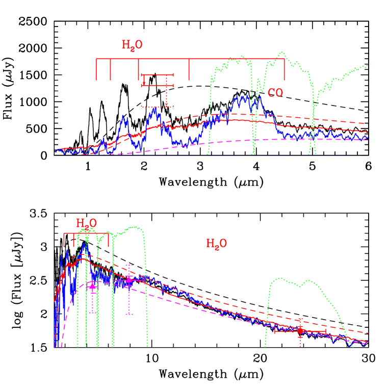
Figure 1: Theoretical spectra of HD209458b. The upper panel shows the 1 to 6 micron window which is expected to contain many H₂O absorption features, and the lower panel shows the spectrum from 1 to 30 microns with log flux on the y axis. Black curve: model 1, $T_{eq}=1700$ K, $f=2$ cloud-free model; blue curve: model 2, $T_{eq}=1450$ K, $f=1$ cloud-free model; red curve: model 3, $T_{eq}=1420$ K, $f=1$ cloudy model. Note how the red curve has very weak absorption bands. The dashed curves show blackbody spectra with $T=1700$ K (black curve) and $T=1430$ K (red curve); HD209458b data points (red solid error bars 1$\sigma$, red dotted error bars 3$\sigma$) are shown as follows. IRTF $\Delta F_{2.2\mu{\rm m}}$ upper limit: the absorption band depth on either side of the 2.2 $\mu$m flux peak must be smaller than the vertical difference between the horizontal bars shown (indicated by the arrows). Because $\Delta F_{2.2\mu{\rm m}}$ is a relative measurement, these horizontal bars can be moved along the y axis. Spitzer MIPS 24$\mu$m point is shown. A hot blackbody is ruled out by the MIPS data, while model 1 ($T_{eq}=1700$ K) is ruled out by $\Delta F_{2.2\mu{\rm m}}$. Spitzer IRAC TrES-1 4.5$\mu$m and 8$\mu$m data are scaled for comparison with HD209458b (magenta triangles and error bars). A $T=1060$ K blackbody (magenta dashed curve) is shown that fits the IRAC data. The renormalized Spitzer IRAC and MIPS band passes are shown as green dotted lines.

Figure 2: The dayside $T_{eq}$ as a function of $A_{B}$ for different values of $f$ (see equation 1). Top panel: $T_{eq}$ for the HD209458 system parameters. The 24 $\mu$m brightness temperature $T_{24}=1130$ K is shown (dash-dot line); if $T_{eq}=T_{24}$ the planet must have a very high Bond albedo. Bottom panel: $T_{eq}$ for the TrES-1 system parameters. The Spitzer IRAC measured brightness temperature of 1050 K is shown (dash-dot line). If $T_{eq}>1200$ K, $f=1$ models are ruled out. Although the measured brightness temperatures for HD209458b and TrES-1 are similar (albeit measured at different wavelengths), values of $T_{eq}$ as a function of $A_{B}$ show that the viable range of planet equilibrium temperature are quite different.

Figure 4: The photosphere and atmospheric circulation. Left panel: Pressure (as a proxy for altitude) at the planetary photosphere as a function of wavelength. (We define the photosphere at an optical depth of 2/3.) The f=2 cloud-free model (model 1) is shown as the solid curve, the f=1 cloudy model (model 3) is shown as the dashed one. Right panel: the altitude dependence of the ratio of the radiative to advective timescales $\tau_{\rm rad}/\tau_{\rm adv}$. A windspeed $U$ of 1000 m/s was adopted for illustration; the ratio scales linearly with $U$ so that other values can be considered. See text for discussion.

References

- Ackerman & Marley (2001) Ackerman, A. S. & Marley, M. S. 2001, ApJ, 556, 872
- Allende Prieto et al. (2002) Allende Prieto, C., Lambert, D. L., & Asplund, M. 2002, ApJ, 573, L137
- Alonso et al. (2004) Alonso, R., Brown, T. M., Torres, G., Latham, D. W., Sozzetti, A., Mandushev, G., Belmonte, J. A., Charbonneau, D., Deeg, H. J., Dunham, E. W., O’Donovan, F. T., & Stefanik, R. P. 2004, ApJ, 613, L153
- Anders & Grevesse (1989) Anders, E. & Grevesse, N. 1989, Geochim. Cosmochim. Acta, 53, 197
- Barman et al. (2001) Barman, T. S., Hauschildt, P. H., & Allard, F. 2001, ApJ, 556, 885
- Bodenheimer et al. (2003) Bodenheimer, P., Laughlin, G., & Lin, D. N. C. 2003, ApJ, 592, 555
- Borysow et al. (2001) Borysow, A., Jørgensen, U. G., & Fu, Y. 2001, JQSRT, 68, 235
- Brown et al. (2001) Brown, T. M., Charbonneau, D., Gilliland, R. L., Noyes, R. W., & Burrows, A. 2001, ApJ, 552, 699
- Burrows et al. (2005) Burrows, A., Hubeny, I., & Sudarsky, D. 2005, submitted to ApJ, astro-ph/0503522
- Burrows et al. (2004) Burrows, A., Sudarsky, D., & Hubeny, I. 2004, in AIP Conf. Proc. 713: The Search for Other Worlds, 143–150
- Chamberlain & Hunten (1987) Chamberlain, J. W. & Hunten, D. M. 1987, Orlando FL Academic Press Inc International Geophysics Series, 36
- Charbonneau et al. (2000) Charbonneau, D., Brown, T. M., Latham, D. W., & Mayor, M. 2000, ApJ, 529, L45
- Charbonneau et al. (2002) Charbonneau, D., Brown, T. M., Noyes, R. W., & Gilliland, R. L. 2002, ApJ, 568, 377
- Charbonneau et al. (2005) Charbonneau, D., et, & al. 2005, ApJ, in press
- Cho et al. (2003) Cho, J. Y.-K., Menou, K., Hansen, B. M. S., & Seager, S. 2003, ApJ, 587, L117
- Cody & Sasselov (2002) Cody, A. M. & Sasselov, D. D. 2002, ApJ, 569, 451
- Cooper & Showman (2005) Cooper, C. S. & Showman, A. P. 2005, submitted to ApJL, astro-ph/0502476
- Cooper et al. (2003) Cooper, C. S., Sudarsky, D., Milsom, J. A., Lunine, J. I., & Burrows, A. 2003, ApJ, 586, 1320
- de Pater & Lissauer (2001) de Pater, I. & Lissauer, J. 2001, Planetary Sciences (Planetary Sciences, by Imke de Pater and Jack Lissauer. Cambridge University Press, 2001, 544 pp.)
- Deming et al. (2005a) Deming, D., Brown, T. M., Charbonneau, D., Harrington, J., & Richardson, J. L. 2005a, ApJ, in press
- Deming et al. (2005b) Deming, D., Seager, S., Richardson, L. J., & Harrington, J. 2005b, Nature, 111, 111
- Fortney et al. (2005) Fortney, J. J., Marley, M. S., Lodders, K., Saumon, D., & Freedman, R. 2005, submitted to ApJL
- Goldreich & Soter (1966) Goldreich, P. & Soter, S. 1966, Icarus, 5, 375
- Gonzalez et al. (2001) Gonzalez, G., Laws, C., Tyagi, S., & Reddy, B. E. 2001, AJ, 121, 432
- Guillot & Showman (2002) Guillot, T. & Showman, A. P. 2002, A&A, 385, 156
- Henry et al. (2000) Henry, G. W., Marcy, G. W., Butler, R. P., & Vogt, S. S. 2000, ApJ, 529, L41
- Iro et al. (2005) Iro, N., Bezard, B., & Guillot, T. 2005, A&A, in press
- Jørgensen et al. (2000) Jørgensen, U. G., Hammer, D., Borysow, A., & Falkesgaard, J. 2000, A&A, 361, 283
- Kuchner & Seager (2005) Kuchner, M. & Seager, S. 2005, ApJ, submitted
- Kurucz (1992) Kurucz, R. L. 1992, in IAU Symp. 149: The Stellar Populations of Galaxies, 225–+
- Laughlin et al. (2005) Laughlin, G., Marcy, G. W., Vogt, S. S., Fischer, D. A., & Butler, R. P. 2005, ApJ, submitted
- Liang et al. (2003) Liang, M., Parkinson, C. D., Lee, A. Y.-T., Yung, Y. L., & Seager, S. 2003, ApJ, 596, L247
- Lodders (2004) Lodders, K. 2004, ApJ, 611, 587
- Lodders & Fegley (1997) Lodders, K. & Fegley, B. 1997, in American Institute of Physics Conference Series, 391–+
- Mazeh et al. (2000) Mazeh, T., Naef, D., Torres, G., Latham, D. W., Mayor, M., Beuzit, J., Brown, T. M., Buchhave, L., Burnet, M., Carney, B. W., Charbonneau, D., Drukier, G. A., Laird, J. B., Pepe, F., Perrier, C., Queloz, D., Santos, N. C., Sivan, J., Udry, S., & Zucker, S. 2000, ApJ, 532, L55
- Menou et al. (2003) Menou, K., Cho, J. Y.-K., Seager, S., & Hansen, B. M. S. 2003, ApJ, 587, L113
- Rayner et al. (2003) Rayner, J. T., Toomey, D. W., Onaka, P. M., Denault, A. J., Stahlberger, W. E., Vacca, W. D., Cushing, M. C., & Wang, S. 2003, PASP, 115, 362
- Richardson et al. (2003) Richardson, L. J., Deming, D., & Seager, S. 2003, ApJ, 597, 581
- Seager (1999) Seager, S. 1999, Ph.D. Thesis
- Seager et al. (2000) Seager, S., Whitney, B. A., & Sasselov, D. D. 2000, ApJ, 540, 504
- Showman & Guillot (2002) Showman, A. P. & Guillot, T. 2002, A&A, 385, 166
- Sudarsky et al. (2003) Sudarsky, D., Burrows, A., & Hubeny, I. 2003, ApJ, 588, 1121
- Visscher & Fegley (2004) Visscher, C. & Fegley, B. 2004, AAS/Division for Planetary Sciences Meeting Abstracts, 36,
- Walker et al. (2003) Walker, G., Matthews, J., Kuschnig, R., Johnson, R., Rucinski, S., Pazder, J., Burley, G., Walker, A., Skaret, K., Zee, R., Grocott, S., Carroll, K., Sinclair, P., Sturgeon, D., & Harron, J. 2003, PASP, 115, 1023