Observation of small scale structure using sextupole lensing

Abstract

Weak gravitational lensing seeks to determine shear by measuring induced quadrupole (elliptical) shapes in background galaxy images. Small impact parameter (a few kpc) gravitational lensing by foreground core masses between $2\,10^{9}\mbox{ and }\,2\,10^{12}M_{\odot}$ will additionally induce a sextupole shape with the quadrupole and sextupole minima aligned. This correlation in relative orientation of the quadrupole and sextupole provides a sensitive method to identify images which have been slightly curved by lensing events. A general theoretical framework for sextupole lensing is developed which includes several low order coefficients in a general lensing map. Tools to impute map coefficients from the galaxy images are described and applied to the north Hubble deep field. Instrumental PSFs, camera charge diffusion, and image composition methods are modelled in the coefficient determination process. Estimates of Poisson counting noise for each galaxy are used to cut galaxies with signals too small to reliably establish curvature. Curved galaxies are found to be spatially clumped, as would be expected if the curving were due to small impact parameter lensing by localized ensembles of dark matter haloes. Simulations provide an estimate of the total required lensing mass and the acceptable mass range of the constituent haloes. The overdensities and underdensities of visible galaxies and their locations in the Hubble foreground is found to be consistent with our observations and their interpretation as lensing events.

1 Introduction

Weak gravitational lensing methods [for review see (Bartelmann and Schneider, 1999; Mellier, 1998; Hoekstra, Yee, and Gladders, 2002) and references therein] allow one to investigate the evolution of matter clustering and the growth of large-scale structure (Wittman et al., 2000; Mellier et al., 2002), and thus probe the properties of both dark energy and dark matter. It is a unique way to investigate both the past and future of the universe. Structure growth is understood as the growth of the matter density fluctuations predicted by inflationary cosmology and dark energy evolution (for review see (Peebles, 1994)), hence the structure of density fluctuations provides information about inflationary scenarios (Huterer and Turner, 2000; Huterer, 2001; Linder and Jenkins, 2003). On the other hand, the matter distribution measurements give bounds on the dark energy equation of state, allowing one to predict the future of the universe (Linde, 2002; Kallosh and Linde, 2003; Kallosh et al., 2003).

The traditional weak gravitational lensing techniques (Kaiser, 2000), which locate and quantify the large clumps of matter such as clusters of galaxies (visible or dark) with $10^{14}\,M_{\odot}$, are not sensitive to the substructure of large clusters or to smaller groups and clumps of matter. We present here a new method designed to detect the presence of smaller clumps. We have applied the method to the north Hubble deep field and have seen a signal which has the features we were expecting. We call this “sextupole lensing”, since it involves the measurement of the quadrupole and sextupole lensing strengths, and may be extended to other sextupole-order and higher terms as well.

Sextupole-lensing strengths lie between strong and weak lensing since these lensing events must yield both quadrupole and sextupole moments the order of the background noise. In comparision, the induced quadrupole moment in weak lensing can be smaller than the background noise and in strong lensing the magnitude of the lensing shear parameter is close to unity.

In the multipole-lensing view, the familiar strong-lensing arclets (Bartelmann and Schneider, 1999; Mellier, 1998) are an example of the general property that the nonlinear 1/r deflections of a light stream passing a mass concentration will produce, relative to the stream centroid, a full complement of moments. The curving seen in the arclet can be understood as the correlated superposition of a quadrupole and sextupole moment, with the length of the arclet usually is determined by the local strength of the octupole moment.

  

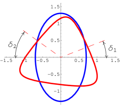
Figure 1: ”Curved” and ”Aligned” galaxies. $\delta=\delta_{1}$ if $|\delta_{1}|<30^{\circ}$, else $\delta=\delta_{2}$. $-30^{\circ}\leq\delta\leq 30^{\circ},$ where $\delta\sim 0^{\circ}$ for ”curved” and $\delta\sim\pm 30^{\circ}$ for ”aligned” galaxies.

The typical cluster identifiable through weak lensing, has a mass of 10¹⁴ solar masses and a radius of about 500 kpc. Since the strength of the quadrupole kick, responsible for the ellipticity, is proportional to the mass and falls off like 1/r², one could get the same induced quadrupole moment in a light stream positioned 5 kpc from an object of 10¹⁰ solar masses. In the latter example, since the sextupole moment varies as 1/r³, the sextupole moment becomes 100 times stronger, becoming as large as the intrinsic sextupole moments of background galaxies. It occurred to us that if ensembles of dark matter contain an abundance of lower-mass clumps, the light streams passing through them might occasionally pass close to a 10⁹ to 10¹¹ solar mass object producing an observable sextupole moment in the image (Irwin and Shmakova, 2003a). Since such “close-encounter” lensing has an alignment of the quadrupole and sextupole moments, a signal for ensembles of dark matter containing a population of lower mass objects, would be evident as spatial correlations in the orientation of the sextupole with respect to the quadrupole moments (“a spatial correlation of an angular correlation”).

Additionally, if the light stream penetrates a mass clump at a location where the mass gradient is non-zero, another 3rd order moment, like the sextupole moment but with a rotational dependence of a dipole moment, is created. This moment, which we call the gradient moment, would be correlated in the same manner.

Let us begin with the simple case of a concentrated point mass. The $1/r$ deflection of a light stream may be expanded in a power series. With a dark matter clump at the origin, and the beam centroid at position $x_{0}$, the kick $\Delta x^{\prime}$ is given as

$$\Delta x^{\prime}=-\frac{4MG}{x}=-\frac{4MG}{x_{0}+\Delta x}=-\frac{4MG}{x_{0}}\left[1-\frac{\Delta x}{x_{0}}+\left(\frac{\Delta x}{x_{0}}\right)^{2}+...\right].$$ (1)

$\Delta x$ indicates the offset from the centroid within the light stream. Each term in the power series is down from the previous term by the fraction $\frac{\Delta x}{x_{0}}$. In other words, to see the effects of higher order terms, the impact parameter can be only a small multiple of the light-stream width.

This power series expansion can be generalized to yield the kick in both coordinates:

$$\Delta x^{\prime}+i\Delta y^{\prime}=-\frac{4MG}{x_{0}+(\Delta x-i\Delta y)}=-\frac{4MG}{x_{0}}\left[1-\frac{\Delta x-i\Delta y}{x_{0}}+\left(\frac{\Delta x-i\Delta y}{x_{0}}\right)^{2}+...\right].$$ (2)

Concentrating on the linear term, one sees for example that the horizontal kick is defocussing, while the vertical kick is focusing. The image appears larger in the focussed direction and smaller in the defocussed direction, hence the linear term changes a circle into an ellipse. It is a general feature that the image distortions have the opposite sign of the map coefficients.

Equation 2 may equally well be written in polar coordinates:

$$\Delta x^{\prime}+i\Delta y^{\prime}=-\frac{4MG}{x_{0}}\left[1-\frac{r}{x_{0}}e^{-i\theta}+\left(\frac{r}{x_{0}}\right)^{2}e^{-i2\theta}+...\right].$$ (3)

The 2nd-order term is the sextupole term. For $\theta=0$ the deflections of the 1st- and 2nd-order terms have the opposite sign, hence the quadrupole is minimum there and the sextupole term is maximum. For $\theta=\pi$ the quadrupole has its other minimum and the sextupole also has a minimum. To the right in fig. 1 are shown the superposition of quadrupole and sextupole distortions for two distinct orientations of the sextupole moment with respect to the quadrupole moment. It is the curved shape that would arise from a lensing event.

The plan we will follow is to measure the quadrupole and sextupole shape of all galaxies, classify each galaxy according to whether it is “curved”, “mid-range” or “aligned”, and examine the distribution of “curved” galaxies on the sky to determine if such galaxies are randomly distributed or unusually clumped.

The remaining sections within this paper are : 2. Lensing maps which introduces the general concept of a nonlinear map, and derives its coefficients for lensing from a general mass distribution arranged on a single plane. Examples of a point mass and a Gaussian radial distribution are provided. 3. Extraction of map coefficients from images, describes three increasingly sophisticated methods for inferring the nonlinear map coefficients from images. The first method is based on image moments, the second uses the best fit of a mapped (initially symmetric) galaxy shape parameterized in a simple form. The third method expands upon the second method to include effects of the point-spread function, charge diffusion in the camera, and important features of the image composition process.

4. Galaxy properties describes the selection of galaxies in the Hubble deep fields and their size and intensity. 5. Quadrupole coefficient measurements presents the results of three methods of map determination to measure the quadrupole coefficient. An analytical estimate for the noise in the quadrupole coefficient, based on Poisson noise of the galaxy image, is presented and noise cuts are implemented. 6. Sextupole coefficient measurements presents the analogous results for the sextupole. The distribution in the angle between quadrupole minimum and sextupole minimum, distinguishing “curved”, “mid-range”, and “aligned” galaxies, is presented.

7. Clumping probabilities employs a “nearest neighbors” analysis to quantify the probability of obtaining the observed spatial distribution of “curved” galaxies in the field if it were to arise randomly. Both “curved” and “aligned” and galaxies are shown to be more clumped than randomly chosen subsets.

8. Dark matter lensing? estimates the mass of the ensembles required to obtain the observed clumping. The total mass and constituent mass are discussed. Lensing by overdensities in dark matter foregrounds is proposed. 9. Systematic effects addresses possible systematic sources of clumping, such as correlated curvature originating with the background galaxies themselves, or correlated curvature from an uncompensated residual of the point-spread function. Section 10. Summary summarizes the paper.

2 Lensing maps

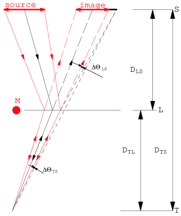
Figure 2: A diagram showing 3 light rays from a source image scattered by a single concentrated mass. The relationship $D_{TS}\Delta\theta_{TS}=D_{LS}\Delta\theta_{LS}$ expresses the observed displacement angle in terms of the actual deflection angle for one ray of the image. Distances are at the epoch of the lensing deflection.

Fig. 2 shows rays from a distant background galaxy being deflected by a mass concentration. The apparent image, as seen by the telescope, is defined by an intensity function which depends only on the angle of each ray as it enters the telescope. Following a ray backwards, toward the apparent image, it is deflected by mass distributions, but is known to depart somewhere from the source galaxy. The ray will have a definite position and angle at the source galaxy (measured relative to the position and angle of the centroid ray). This map from telescope variables to source variables will be symplectic since the light geodesics are described by a Hamiltonian. From the point of view of the galaxy, all rays traced backward from the telescope come from the same point. Hence the two angles (or equivalently, the focal plane coordinates) at the telescope uniquely describe the trajectory through space and the initial position $x_{S}$ and $y_{S}$ (and angle ${x}^{\prime}_{S}$ and ${y}^{\prime}_{S}$) at the galaxy. Thus the “backwards” map can be written as a set of 4 functions $x_{S}(x_{T},y_{T}),\;y_{S}(x_{T},y_{T}),\;{x}^{\prime}_{S}(x_{T},y_{T}),\;\mbox{and }{y}^{\prime}_{S}(x_{T},y_{T})$, where “T” designates “telescope” and “S” designates “source”. The coordinate system for both the source and telescope images will be taken to be location on the focal plane. The position of the centroid trajectory is taken to be identical for both images, i.e. the dipole kick suffered by the image as a whole is ignored. Only under special circumstances, such as strong lensing, will a ray leaving the telescope at different angles arrive at the same point on the source galaxy. We will not consider such cases and hence will be able to drop the two functions ${x}^{\prime}_{S}\mbox{ and }{y}^{\prime}_{S}$ and concern ourselves with regions for which the determinant

$${\Big{|}}\begin{array}[]{cc}{\frac{\partial x_{S}}{\partial x_{T}}}&{\frac{\partial x_{S}}{\partial y_{T}}}\\ {\frac{\partial y_{S}}{\partial x_{T}}}&{\frac{\partial y_{S}}{\partial y_{T}}}\\ \end{array}{\Big{|}}>0.$$ (4)

The two functions $x_{S}(x_{T},y_{T})\mbox{ and }y_{S}(x_{T},y_{T})$ can be combined into one complex function by defining $w_{S}=x_{S}+iy_{S}$. This complex function can be written in terms of the variables $w_{T}=x_{T}+iy_{T}$ and $\bar{w}_{T}=x_{T}-iy_{T}$ by substituting $x_{T}=\frac{1}{2}\left({w_{T}+\bar{w}_{T}}\right)$ and $y_{T}=\frac{1}{2i}\left({w_{T}-\bar{w}_{T}}\right)$. The map equations can then be written as the single function $w_{S}(w_{T,}\bar{w}_{T}).$ Since the transverse width of the light stream will be small compared to characteristic dimensions of the variations of the lensing mass distributions, we may expand this function in a power series about the stream centroid:

$$w_{S}(w_{T},\bar{w}_{T})=w_{T}+\sum\limits_{n,m=0}^{\infty}{a_{nm}w_{T}^{n}}\bar{w}_{T}^{m}.$$ (5)

The significance of the variables $w$ and $\bar{w}$ rests on the fact that products and powers of them are rotation eigenfunctions. It follows that the terms in the expansion for $w_{S}$ have a simple interpretation. The $1+a_{10}$ combination represents a simple rotation and scaling, the $a_{01}$ term is a quadrupolar distortion, the $a_{02}$ term is a sextupolar distortion, the $a_{03}$ term is an octupolar distortion, the $a_{20}$ term is a cardioid-like distortion, and the $a_{11}$ term is an $r^{2}$-dependent translation of circles, and so on. We will be concerned primarily with the terms $a_{01}$, $a_{02}$, $a_{03}$, and $a_{20}$ and refer to them more simply by the letters, $a,\;b,\;c,\mbox{ and }\bar{d}$, respectively. As we show in the following paragraph, for a map arising from mass distributed on a plane, $a_{10}$ is necessarily real and $a_{11}=2\bar{a}_{20}=2{d}.$ Note that the coefficients $b,\;c,\mbox{ and }d$ have dimensions. Since we are using focal-plane position as the coordinate system, units will usually be given in terms of the pixel grid on that plane.

In this paper we limit ourselves to maps arising from mass distributions which can adequately be represented by mass projected onto a single plane (which we will refer to as the lensing plane). To determine the Green’s function for this case, consider the effect of a point mass. A light stream passing at distance $r$ will be deflected radially by the angle $\Delta{r}^{\prime}=-\frac{4MG}{r}$. The potential for such a kick, the sought Green’s function, is $2\Phi_{\delta}=4MG\,Ln\left[r\right]$. This is just the Green’s function for the 2 dimensional Laplace equation, $\nabla^{2}\Phi=4\pi G\rho$, where $\rho$ is the mass density function.

In accord with the variables chosen for the map, we expand the solution to Laplace’s equation in the variables $w=x+iy$ and $\bar{w}=x-iy$. Variables without subscripts are taken to lie in the lensing plane. To enable power series expansions, it is useful to introduce derivative operators $\partial\equiv\frac{\partial}{\partial w}\equiv\frac{1}{2}\left[{\frac{\partial}{\partial x}-i\frac{\partial}{\partial y}}\right]$ and $\bar{\partial}\equiv\frac{\partial}{\partial\bar{w}}\equiv\frac{1}{2}\left[{\frac{\partial}{\partial x}+i\frac{\partial}{\partial y}}\right]$, which have the desired property that $\partial w=\bar{\partial}\bar{w}=1$ and $\partial\bar{w}=\bar{\partial}w=0$.

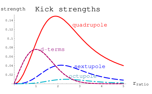
Figure 3: Relative strength of the quadrupole, sextupole, octupole, and cardioid-like kicks within a Gaussian clump. The horizontal axis is the radius divided by the rms lens radius.

Using these variables, the power series expansion for the potential is $\Phi=\sum\limits_{n,m=0}^{\infty}\frac{1}{n!m!}\Phi_{nm}w^{n}\bar{w}^{m}$ where $\Phi_{nm}={\partial}^{n}\bar{\partial}^{m}\Phi$ evaluated at $w=w_{0}$. The reality condition on $\Phi$ implies relationships among these coefficients. For example, the $\Phi_{nn}$ are real and $\Phi_{nm}=\overline{\Phi_{mn}}$. If both $n$ and $m$ are greater than or equal to 1, the term will be proportional to the density or a derivative of the density, since $\Phi_{11}=\frac{1}{4}\nabla^{2}\Phi=\pi G\rho$. The two components of the kick, given in the form $\Delta x^{\prime}+i\Delta y^{\prime}$, are contained in the single equation,

$$\Delta{w}^{\prime}=-2\,\bar{\partial}{\left(2\Phi\right)}.$$ (6)

The geometry of fig. 2 implies $w_{S}=w_{T}+D_{LS}\Delta w^{\prime}(w,\bar{w})$ with $w=\frac{D_{TL}}{D_{TS}}w_{T}$. Thus for a general potential the map coefficients are given by

$$a_{10} = -4D_{LS}\frac{D_{TL}}{D_{TS}}\Phi_{11}=-4\pi GD_{LS}\frac{D_{TL}}{D_{TS}}\rho,$$ (7)

$$a = -4D_{LS}\frac{D_{TL}}{D_{TS}}\Phi_{02},$$ (8)

$$b = -4D_{LS}\left({\frac{D_{TL}}{D_{TS}}}\right)^{2}\frac{1}{2}\Phi_{03},$$ (9)

$$c = -4D_{LS}\left({\frac{D_{TL}}{D_{TS}}}\right)^{3}\frac{1}{3!}\Phi_{04},\,\mbox{ and }$$ (10)

$$d = -4D_{LS}\left({\frac{D_{TL}}{D_{TS}}}\right)^{2}\Phi_{12}=-2\pi GD_{LS}\left({\frac{D_{TL}}{D_{TS}}}\right)^{2}\bar{\partial}\rho.$$ (11)

The map coefficients for the point source may be found by evaluating the derivatives of $2\Phi_{\delta}=4MG\,Ln\left[r\right]=2MG\,Ln\left[w\bar{w}\right]$:

$$a_{\delta} = D_{LS}\frac{D_{TL}}{D_{TS}}\frac{4MG}{\bar{w}_{0}^{2}},$$ (12)

$$b_{\delta} = -D_{LS}\left({\frac{D_{TL}}{D_{TS}}}\right)^{2}\frac{4MG}{\bar{w}_{0}^{3}},$$ (13)

$$c_{\delta} = D_{LS}\left({\frac{D_{TL}}{D_{TS}}}\right)^{3}\frac{4MG}{\bar{w}_{0}^{4}},\,\,\mbox{and}$$ (14)

$$d_{\delta} = a_{10\,\delta}=0.$$ (15)

The map coefficients can be easily found for any symmetric mass distribution by using Gauss’ law ( $\frac{\partial\Phi}{\partial r}=\frac{2M(r)G}{r}=\frac{4\pi G}{r}\int\limits_{0}^{r}\rho(r^{\prime})r^{\prime}dr^{\prime}$) and the relationship $\bar{\partial}\Phi(r)=\frac{w}{2r}\frac{\partial\Phi(r)}{\partial r}.$ For a plot of the coefficient strengths in the case of a Gaussian mass distribution see fig. 3.

3 Extraction of map coefficients from images

We use three distinct methods to estimate lensing map coefficients: $1)$ a moment method, $2)$ a radial-fit method, and $3)$ a model method that takes into account the point-spread function (PSF), the diffusion of charge between camera pixels, the dithering of pointing, and drizzle of photon counts onto the final pixel grid.

The moment method has the advantage of simplicity, but because the images are necessarily truncated its accuracy is compromised as a result of edge effects and an inherent ambiguity in including the effect of the PSF. Furthermore, it does not bring into play the knowledge that moments derived from the action of lensing will have a radial strength proportional to the derivative of the radial profile of the galaxy. The radial-fit method overcomes these shortcomings. When we take into account the PSF and other known processes that distort galaxy images, namely the charge diffusion and image composition, we refer to the method as the model method. The model method begins with a parameterized radial profile of the source galaxy and in addition models the PSF, diffusion and other image composition processes. This latter method is limited by the imperfect knowledge of the features it seeks to include (such as PSF and charge diffusion), plus of course, the noise inherent in background galaxy shapes and photon counting noise.

We wish to emphasize that the radial-fit and model methods do not contain an implicit assumption of azimuthal symmetry for the background galaxies. One can imagine applying either of these methods to an unlensed galaxy, and finding non-zero map coefficients, $a_{S}$ and $b_{S}$. Then if that same galaxy is later lensed one obtains, $a=a_{S}+a_{L}$ and $b=b_{S}+b_{L}$, where $a_{L}$ and $b_{L}$ are the coefficients of the linear and quadratic terms in the lensing map. For a proof of this see the appendix.

3.1 Moment method

Image moments are defined by the integrals $M_{nm}=\int w^{n}\bar{w}^{m}i(x,y)dxdy$, where $i(x,y)$ is the light-intensity function normalized to unit integral. According to the notation introduced in the previous section, we distinguish the original source galaxy intensity by the subscript $S$ and the intensity as observed at the telescope by the subscript $T$. Because of the symplectic nature of the lensing map, these intensities are related to one another by $i_{S}(x_{S},y_{S})\,dx_{S}dy_{S}=i_{T}(x_{T},y_{T})\,dx_{T}dy_{T}$. Using this relationship one can relate the moments of the source to the moments of the observed image through

$$M_{nm}^{S} = \int w_{S}^{n}\bar{w}_{S}^{m}\,i_{S}(x_{S},y_{S})dx_{S}dy_{S}$$ (16)

$$= \int(w_{T}+\Delta w)^{n}(\bar{w}_{T}+\overline{\Delta w})^{m}i_{T}(x_{T},y_{T})\,dx_{T}dy_{T},$$ (17)

where $\Delta w=a\bar{w}_{T}+b\bar{w}_{T}^{2}+c\bar{w}_{T}^{3}+2d{\kern 1.0pt}w_{T}\bar{w}_{T}+\bar{d}{\kern 1.0pt}w_{T}^{2}$.

Inserting this expression for $\Delta w$ into the expression for $M_{20}^{S}$ one can find the following equation for the quadrupole map coefficient:

$$\begin{array}[]{c}M_{20}^{S}=\int{\left({w_{T}+a\bar{w}_{T}+...}\right)^{2}\,}i_{T}(x_{T},y_{T})dx_{T}dy_{T}\approx M_{20}^{T}+2aM_{11}^{T}+a^{2}M_{02}^{T}.\end{array}$$ (18)

Since the moments on the right hand side of this equation can be measured from the telescope image (neglecting problems with truncation errors), one obtains a quadratic equation for $a$ depending on the value of $M_{20}^{S}$, which, lacking any information of its value, is usually set equal to zero. Since $w\bar{w}=r^{2}\mbox{ it follows that }M_{11}^{T}$ is the mean square radius of the telescope image. Solving for $a$,

$$a\approx-\frac{\Delta M_{20}}{2M_{11}^{T}}\,\frac{2}{1+\sqrt{1+\frac{\Delta M_{20}\bar{M}_{20}}{M_{11}^{T2}}}},$$ (19)

where $\Delta M_{nm}\equiv M_{nm}^{T}-M_{nm}^{S}.$

Likewise an equation for the sextupole moment may be found by inserting the expression for $\Delta w$ into the expression for $M_{30}^{S}$ obtaining

$$M_{30}^{S}\approx M_{30}^{T}+3b\,M_{22}^{T}+3a\,M_{21}^{T}+\ldots\mbox{ whence }b\,\approx-\frac{\Delta M_{30}}{3M_{22}^{T}}-\frac{a\,M_{21}^{T}}{M_{22}^{T}}\quad.$$ (20)

Similarly the expression for $c$ is derived from

$$M_{40}^{S}\approx M_{40}^{T}+4c\,M_{33}^{T}+4a\,M_{31}^{T}+6a^{2}M_{22}^{T}+\ldots\mbox{ yielding }c\,\approx-\frac{\Delta M_{40}}{4M_{33}^{T}}-\frac{a\,M_{31}^{T}}{M_{33}^{T}}-\frac{3a^{2}\,M_{22}^{T}}{2M_{33}^{T}}.$$ (21)

And to get an expression for the d-term, we insert $\Delta w$ into an expression for $M_{21}^{S}$ resulting in

$$M_{21}^{S}=M_{21}^{T}+2a\bar{M}_{21}^{T}+\bar{a}M_{30}^{T}+5d\,M_{22}^{T}+\ldots\mbox{ yielding }d\approx-\left[\Delta M_{21}^{T}+2a\bar{M}_{21}^{T}+\bar{a}M_{30}^{T}\right]\frac{1}{5M_{22}^{T}}.$$ (22)

If the image were not truncated it would be possible to extend this method to expressions for the moments in the presence of a PSF. The resulting corrections to the moment equations provide insight into the magnitude of PSF corrections. Intensity functions which have been convolved with the PSF and moments derived from these functions will be designated by a “^∧”. Let $p$ be the point-spread function. Then

$$\hat{M}_{nm}^{T} = \int{w_{T}^{n}\bar{w}_{T}^{m}\,\hat{i}_{T}(x_{T},y_{T})dx_{T}dy_{T}}=\int{\int{w_{T}^{n}\bar{w}_{T}^{m}\,p(\vec{r}_{T}-\vec{{r}^{\prime}}_{T})\,i_{T}({\vec{r}}^{\prime}_{T})dx_{T}dy_{T}d{x}^{\prime}_{T}d{y}^{\prime}_{T}}}$$

$$= \int{\int{\left({\Delta w_{T}+{w}^{\prime}_{T}}\right)^{n}\left({\Delta\bar{w}_{T}+\bar{{w}^{\prime}}_{T}}\right)^{m}}}p(\Delta\vec{r}_{T})i_{T}({\vec{r}}^{\prime}_{T})d\Delta x_{T}d\Delta y_{T}d{x}^{\prime}_{T}d{y}^{\prime}_{T}.$$

Here $\Delta x_{T}\equiv x_{T}-{x}^{\prime}_{T}$ etc. When the binomial expressions are expanded, the double integral reduces to the sum of a product of single integrals. One finds, for example,

$$\hat{M}_{20}^{T} = M_{20}^{P}+M_{20}^{T},\quad\hat{M}_{30}^{T}=M_{30}^{T}+M_{30}^{P},\quad\hat{M}_{21}^{T}=M_{21}^{T}+M_{21}^{P},$$ (24)

$$\hat{M}_{11}^{T} = M_{11}^{P}+M_{11}^{T},\quad\mbox{and}\quad\hat{M}_{22}^{T}\approx M_{22}^{T}+2M_{11}^{P}M_{11}^{T}+M_{22}^{P}.$$ (25)

In all cases, if the moments of the point-spread function are known, the moments of the original image can be found from the smeared image.

Finally, using the approximations $\hat{a}\equiv-\frac{\hat{M}_{20}^{T}}{2\hat{M}_{11}^{T}}$ and $a^{P}\equiv-\frac{M_{20}^{P}}{2M_{11}^{P}}$ and similar approximations for $\hat{b}$ and $b^{P}$, and using the relationships of eq.24, one can find an approximation for the map coefficients “before PSF”:

$$a=\frac{1}{\lambda_{1}^{T}}\left(\hat{a}-\lambda_{1}^{P}a^{P}\right)\;\;\;\mbox{and}\;\;\;b=\frac{1}{\lambda_{2}^{T}}\left(\hat{b}-\lambda_{2}^{P}b^{P}\right),$$ (26)

where

$$\lambda_{1}^{X}\equiv\frac{M_{11}^{X}}{M_{11}^{T}+M_{11}^{P}}\,;\;\;\mbox{ and }\;\;\lambda_{2}^{X}\equiv\frac{M_{22}^{X}}{M_{22}^{T}+2M_{11}^{T}M_{11}^{P}+M_{22}^{P}}.$$ (27)

3.2 Radial-fit method

We assume a radial profile for the background galaxy of the form

$$F(r_{S}^{2})=(A+Br_{S}^{2}+Cr_{S}^{4})_{{}_{+}}\,e^{-Dr_{S}^{2}}.$$ (28)

This will be adequate since this function must depend only on $r_{S}^{2}$, and we have a parameter ($A$) for the strength at the center of the galaxy, a parameter ($B$) that allows for an arbitrary quadratic behavior at the origin, there is a cut-off parameter ($D$) that reflects the image size , and a parameter ($C$) which can modify the behavior as one approaches the cut-off. The $+$ subscript indicates that if the polynomial has a value less than zero, it is to be set equal to zero. This is necessary to avoid negative intensities, which would be unphysical. Given a centroid, one may numerically determine the radial profile of a galaxy (for example, by dividing each pixel into many smaller pixels), and this may be compared with the fit results. In cases we have examined, the two curves are almost indistinguishable.

For convenience we introduce two additional parameters: each occurrence of $r_{S}^{2}$ is replaced by $(r_{S}/r_{0})^{2}$, and a constant $c_{0}$ multiplies the polynomial.

$$F(r_{S}^{2})=c_{0}(A+Bs+Cs^{2})_{{}_{+}}\,e^{-Ds}\mbox{ with }s=(\frac{r_{S}}{r_{0}})^{2}.$$ (29)

$r_{0}$ is taken to be near the rms size of the source image. By changing the size of $r_{0}$ one can change the size of the image without affecting its shape. The factor $c_{0}$ is introduced so that the shape parameters, which are now dimensionless, have values $A\approx 1$ and $B\mbox{ and }C$ can be compared to unity.

The effect of lensing is contained in the parameters of the map of eq. 5. One replaces each occurrence of $r_{S}^{2}$ by the expression $w_{S}\bar{w}_{S}$.

The parameters of the radial profile and the map are determined by minimizing the L2 norm:

$$\|{i_{F}-i_{T}}\|_{\rho}^{2}=\int{(i_{F}-i_{T})^{2}\,\rho\,dx_{T}dy_{T}}\mbox{, where }i_{F}=F(r_{S}^{2})\,|\frac{\partial w_{S}}{\partial w_{T}}|.$$ (30)

In $i_{F}$, $r_{S}^{2}=w_{S}\bar{w}_{S}$ is understood to be a function of $x_{T}$ and $y_{T}$ through $w_{T}$ and $\bar{w}_{T}$. The $|...|$ is the Jacobian of the transformation between $S$ and $T$ variables. All map variables in the Jacobian occur in 2nd order except for the $d$ variable, which occurs in 1st order. A weight function $\rho$ can be introduced if desired. However, because this technique ignores truncated pixels rather than considering them to be zero, edge effects are inherently smaller compared to the moment method. At each calculation of $i_{F}$ the Jacobian is monitored to see that it is not negative at that or any smaller $r$.

With parameters $a,b,c,$ and $d$ included in the map, then together with the centroid position, $w_{0}$, and the shape parameters $A,B,C,$ and $D$, there are 14 variables to determine. The fit is done in several steps using a multi-dimensional Newton’s method. At each step any subset of the 14 variables are allowed to vary. The curvature matrix for these parameters is computed, then diagonalized and eigenvectors with very small eigenvalues are not allowed to contribute to the function change in that step. The convergence to a minimum is controlled by a parameter step size, which finally is required to be as small as $10^{-15}$.

The map parameters are not strictly orthogonal, but because of their distinct leading angular behavior, they appear to be stable and well determined. We have thoroughly tested the fit program by fitting many generated matrices, starting from a variety of initial conditions. Typically map parameters are reproducible to parts per thousand at typical moderate parameter strengths. The method is less accurate for images with large map parameters.

3.3 Model method

The model method begins by constructing an $i_{F}$ as in the previous subsection (here on .02” pixels) and convolving it with a sub-sampled PSF (also on .02” pixels) as provided by the Tiny Tim program. This convolved image is dropped (25 times) onto a dithered original pixel grid (0.1” pixels). A diffusion kernel,

$$K=\left[\matrix{.025&.05&.025\cr.05&.70&.05\cr.025&.05&.025}\right]$$ (31)

is applied to each resulting image. The image on each original pixel is shrunk to half its size in each dimension, and then “drizzled” to the final Hubble deep field grid (0.04” pixels) according to the intersection of the diminished original pixel area with the pixels in the final grid. We do not attempt to reproduce the actual offsets of the dithers of the original camera. The actual process has 9 dithers whose offsets vary across the field. We are content to capture the main features of the dither, diffusion, and drizzle process. Ultimately one would prefer to avoid the drizzle operation and fit the original dithered images directly. The model method is well suited for that.

An additional complication with the model method comes from the Jacobian condition given the fact that $a$ and $b$ for the fit to the source are typically larger by a factor of about 2 as compared to the radial-fit method. In the case where we are fitting only the $a$ and $b$ map parameters, the Jacobian is given by $1-|a+2b\bar{w_{T}}|^{2}.$ For fixed radius $r$ the condition on positivity for all angles $\theta$ becomes $|a|+2|b|r\leq 1$. We must introduce an additional cut, of the form $|a|+2|b|r_{Max}\leq 1$.

4 Galaxy properties

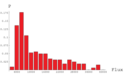
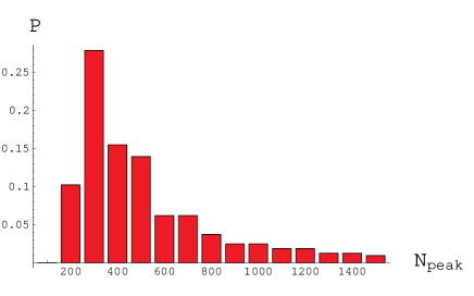
Figure 4: The distribution of total photon counts for all galaxies in the north HDF with $z\geq 0.8$, identified by SExtractor with intensity exceeding $6\sigma_{NF}$, and having a single major maximum (left plot). The photon count of the peak pixel for the same galaxies (right plot).

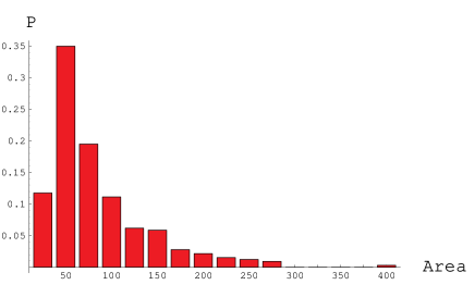
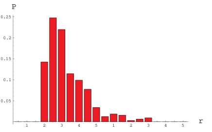
Figure 5: Distribution of galaxy areas (left plot) and distribution of galaxy rms radii (right plot) for the galaxy set described in fig. 4 above.

The software SExtractor (Bertin and Arnouts, 1996) was used to select galaxies from the Hubble deep field and to specify which pixels to include in the image. Galaxies were selected which appeared for both a $4\sigma_{NF}$ and a $6\sigma_{NF}$ threshold option (4 or 6 times the rms noise floor) with the convolution option taken to be the identity. Only galaxies that had been assigned a $z$-value with $z>0.8$ were kept. There were about 569 galaxies so identified in the north field. The images used in our analysis were cut at $6\sigma_{NF}$ and defined to be the dominant simply-connected region.

Galaxy images were transferred to the Mathematica programming environment for inspection where galaxies with more than one maxima were removed. Of the 569 identified galaxies with $z>0.8$, 427 survived this single-max cut. The total photon count and peak height of the surviving galaxies are shown in fig. 4, and the total area and rms radius are shown in fig. 5.

5 Quadrupole coefficient measurements

5.1 Quadrupole coefficients from moment and radial-fit methods

In fig. 6 (left) we compare the distributions of the magnitudes of the quadrupole coefficients using the moment method and the radial-fit method. The range of magnitudes is surprisingly similar. This can only arise if the fit to the radial profile results in an $M_{20}^{T}$ moment that is significantly less than the integrated moment. For if $M_{20}^{T}$ were arising dominantly from the mapping of an originally radial galaxy profile, one can derive a simple analytic expression for the magnitude of this moment, even when truncated. To see this, consider the following expression for one component of $M_{20}^{T}$.

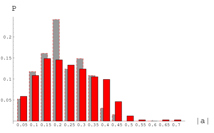
Figure 6: Distribution of the quadrupole map coefficient for all galaxies in the set described in fig. 4, for both the moment method (background) and the radial fit method (foreground)(left plot) and comparison of the angular orientation of the quadrupole map coefficient for the moment method and the radial fit method (right plot).

$$\Re\left[M_{20}^{T}\right] = \int r^{2}cos2\theta\,i_{S}(r_{S}^{2})\,|\frac{\partial w_{S}}{\partial w_{T}}|\,dA$$ (32)

$$\approx \int r^{2}cos2\theta\,\{i_{S}(r^{2})+2r^{2}(a_{x}cos2\theta+a_{y}sin2\theta)\,\frac{di_{S}}{dr^{2}}+...\}\,rdrd\theta$$ (33)

$$\approx 2\pi a_{x}\int r^{4}\frac{di_{S}}{dr^{2}}dr^{2}\approx-2a_{x}\int[i_{S}(r^{2})-i_{S}(r_{T}^{2})]dA=-2a_{x}\underline{M}_{11}^{T}$$ (34)

The integral here is only over the footprint of the truncated image, which for the purposes of this estimate, is assumed to be a disk of radius $r_{T}$. The underline of $M_{11}^{T}$ indicates that the integrand is to be defined as the photon-count-per-pixel in excess of the truncation floor. We will call this an “above-floor” moment. The equation can now be solved for $a_{x}$ with a result which is satisfyingly simple and directly comparable with the result found using the moment method as in eq.18: the denominator $M_{11}^{T}$ is simply replaced by $\underline{M}_{11}^{T}$. Similar results can be found for the other moments, which we summarize here for future reference.

$$a \approx -\frac{M_{20}^{T}}{2\underline{M}_{11}^{T}},\quad\quad\quad\quad b\approx-\frac{M_{30}^{T}}{3\underline{M}_{22}^{T}},$$ (35)

$$c \approx -\frac{M_{40}^{T}}{4\underline{M}_{33}^{T}},\quad\mbox{and}\quad d\approx-\frac{M_{21}^{T}}{9\underline{M}_{22}^{T}-4M_{22}^{T}}.$$ (36)

The irregularity in the expression for $d$ arises from the linear dependence on $d$ in the Jacobian.

Since the “above-floor” expressions for the coefficients may have a significantly smaller denominator than the expressions used in the straight moment method, these “above-floor” estimates for map coefficients could be significantly larger. Based on our results for the radial-fit method, which does insist on such a relationship, one can only draw the conclusion that a part of the moment $M_{20}^{T}$ is not coming from the distortion of the radial profile. This is an interesting result, and indicates that the radial-fit method is indeed an important tool in making such a distinction. We would assert that a substantial amount of noise is projected out with the radial method. This could be important for high-resolution weak-lensing surveys such as SNAP.

The orientation of moments is more important to us than their magnitude. Figure 6 (right) compares the map coefficient orientation of the radial-fit method with the moment method. We would like to establish the orientation of the resultant elliptical shape within $10^{\circ}$. Since the quadrupole map coefficient advances by $2\phi$ as the ellipse rotates by $\phi$, the relevant limit for the determination of $\phi$ is $20^{\circ}$. One can see in fig. 6 that the angle differences between these two methods for the quadrupole map coefficient are often larger than $20^{\circ}$.

5.2 Quadrupole noise estimates

The first formula of eq. 35 can be used to derive a Poisson-noise estimate for the quadrupole coefficient, $a_{fit}$, derived from the fit method. An estimate for the contribution of Poisson noise to $M_{20}$ is required. For each component, this can be obtained from the integral

$$\Re\left[M_{20}^{T}\right] = \frac{\int r^{2}cos2\theta\,\zeta\sqrt{n(r,\theta)}dA}{\int n(r,\theta)dA}\approx\frac{1}{N}\sqrt{\int r^{4}cos^{2}2\theta\,n(r,\theta)dA}\approx\sqrt{\frac{M_{22}^{T}}{2N}}$$ (37)

where $\zeta$ is a stochastic variable, $n(r,\theta)$ is the number of counts for each pixel, and $N$ is the total number of counts for the image. Similar formulae hold for the other map coefficients. We summarize the results:

$$|a_{x\,N}| \approx \sqrt{\frac{M_{22}^{T}}{2N}}\frac{1}{2\underline{M}_{11}^{T}},\quad\quad\quad\quad\quad|b_{x\,N}|\approx\sqrt{\frac{M_{33}^{T}}{2N}}\frac{1}{3\underline{M}_{22}^{T}},$$ (38)

$$|c_{x\,N}| \approx \sqrt{\frac{M_{44}^{T}}{2N}}\frac{1}{4\underline{M}_{33}^{T}},\quad\mbox{and}\quad|d_{x\,N}|\approx\sqrt{\frac{M_{33}^{T}}{2N}}\frac{1}{9\underline{M}_{22}^{T}-4M_{22}^{T}}.$$ (39)

The subscript $x$ indicates that this is an estimate for one component, which could be in any direction of course. It is a minimum estimate, in the sense that only the Poisson counting noise is being included. For example, contributions to the noise from edge effects are not included.

The actual $|a|$ should be large enough so that if the perpendicular component to $a$ was changed by an amount $|a_{x\,N}|$ the angle would change by less than the required resolution on angles. The magnitude of the relative orientation of the quadrupole and sextupole shapes ($\delta$ in fig. 1), runs from $0^{\circ}$ to $30^{\circ}$ . Since we choose to designate “curved” galaxies as those for which $|\delta|<10^{\circ}$, “aligned” galaxies as those for which $|\delta|>20^{\circ}$, and “mid-range” galaxies as the remaining ones, and considering positive as well as negative signs for $\delta$, the regions describing curved and aligned are actually $20^{\circ}$ wide. Hence we may take $10^{\circ}$ (=0.17 rad) as an estimate for the required resolution on $\delta$. Since $\delta$ is the difference between the orientation of the quadrupole and sextupole shapes, the resolution on $\delta$ could be achieved by requiring the sum of the resolution squared of each shape individually to be less than $(0.17)^{2}$ . As the shapes rotates by $\phi$ the quadrupole map coefficient angle changes by $2\phi$ and the sextupole map coefficient angle changes by $3\phi$. Thus this resolution condition on $a_{fit}\mbox{ and }b_{fit}$ could be written

$$\left[\frac{1}{2}\tan^{-1}|\frac{a_{x\,N}}{a_{fit}}|\right]^{2}+\left[\frac{1}{3}\tan^{-1}\big{|}\frac{b_{x\,N}}{b_{fit}}\big{|}\right]^{2}<(0.17)^{2}$$ (40)

We could choose to satisfy this condition by requiring that the quadrupole contribution be less than $6.3^{\circ}$ and the sextupole contribution be less than $7.8^{\circ}$. The quadrupole cut would then be equivalent to requiring that $|a|>4.5|a_{x\,N}|$ and the sextupole cut would be equivalvent to $|b|>2.3|b_{x\,N}|$. The results of the quadrupole cut are shown in fig. 7, where the vertical axis is the quadrupole strength and the horizontal axis is the estimated Poisson noise from eq. 38 for that galaxy. The straight line is the cut condition and galaxies below this line would be rejected as having a signal-to-noise ratio which is too small.

In fig. 8 we show the comparison between the moment and radial-fit methods after this signal-to-noise cut for magnitude distributions and angle distributions. The orientations using the two methods are now in better agreement.

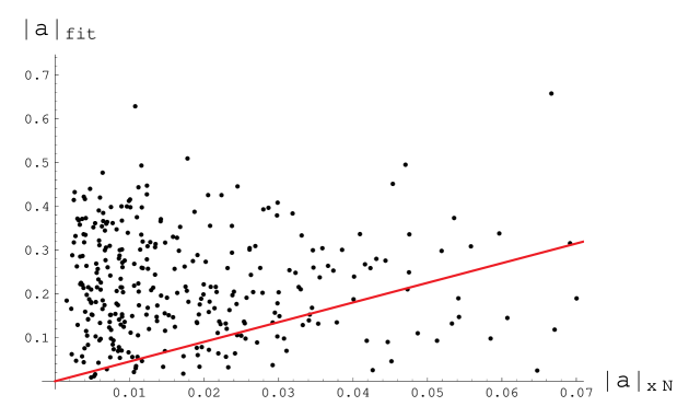
Figure 7: A plot of the quadrupole Poisson noise estimate (horizontal axis) versus the magnitude of the quadrupole coefficient. The galaxies falling below the straight line with slope 4.5 will be cut as having signal-to-noise ratios too small.

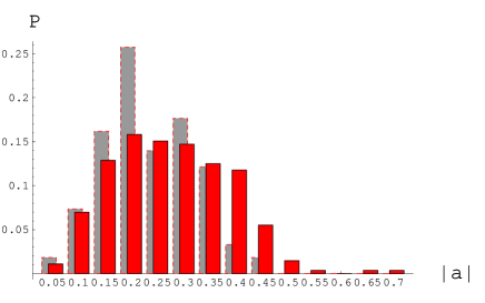
Figure 8: Comparison, after signal-to-noise cut, of the magnitude of the quadrupole map coefficient for both the moment method (background) and the radial fit method (foreground) (left plot) and of the angular orientation of the quadrupole map coefficient for the moment and the radial fit methods (right plot). Compare with fig. 6

5.3 Quadrupole coefficients from the model method

In fig. 9 we show the magnitude of the quadrupole coefficient (left panel) using the model method. Of the 427 selected galaxies having one apparent maximum, 47 resulted in an L2 norm squared ($\|i_{F}-i_{T}\|^{2}$) greater than $0.05$. These galaxies were cut from the sample, for the reason that their shape does not sufficiently well conform to the model we are using to estimate map-coefficient strengths.

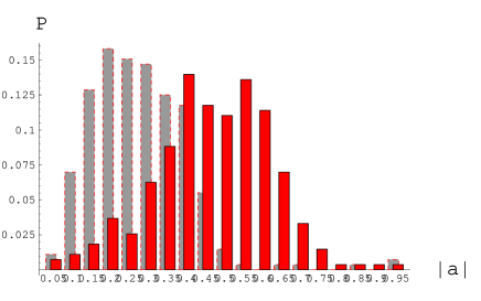
Figure 9: Distribution of the magnitude of the quadrupole map coefficients using the model method (foreground) compared with the radial-fit method (background) (left plot) and of the angular orientation of the quadrupole map coefficient for the model and the radial fit methods (right plot).

The magnitudes of the quadrupole coefficients are clearly larger in the model case than the radial-fit case because the rms size of the source image is smaller. This increase is represented by the factor $1/\lambda_{T}$ in eq. 26.

Figure 9 (right plot) compares the orientations of the quadrupole map coefficient of the radial-fit method with the model method. The differences are now much smaller. The diffusion, being symmetric, will not change the orientation, but the PSF of the Hubble is known to have a substantial quadrupolar component which varies dramatically across the field, frustrating attempts to do weak lensing with the Hubble.

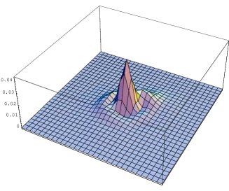
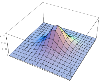
Figure 10: A picture of a Hubble WPFC2 PSF as produced by the Tiny Tim program on the left. The pixel size is 5x smaller than the Hubble camera pixels, in other words 2x smaller than the drizzled HDF pixels (left plot). On the right, the same PSF diffused and drizzled .

An example of a 5x sub-sampled PSF, as obtained from Tiny Tim, is shown in Fig. 10 (left plot). We have specified the the F606 filter at the location of each of the 427 galaxies in our sample. There is typically a diffraction ring at a radius of 2 HDF pixels which contains about 30% of the counts. The radius of the central peak is too small to give significant moments, so the moments of concern arise from the ring.

Fig. 10 (right plot) shows this PSF after it has been dithered, diffused and dropped onto the final Hubble 0.04” grid. We have taken these PSFs which have been dithered, diffused and drizzled, and fit them using the radial fit method. Fig.11 shows the resulting distribution of the magnitude of the quadrupole coefficients (right) as well as their spatial distribution and orientation (left).

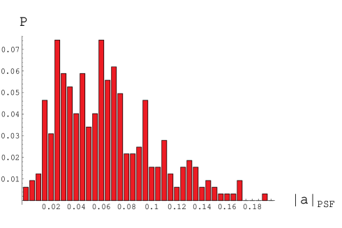
Figure 11: Spatial ellipticity distribution (left) and the quadrupole coefficient magnitude distribution (right) for the 5x subsampled and drizzled Tiny Tim PSFs for the WPFC2 camera on the Hubble.

6 Sextupole coefficient measurement

6.1 Sextupole coefficients from moment and radial-fit methods

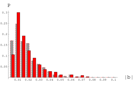
Figure 12: The left plot is a distribution of the magnitude of the sextupole map coefficient, for the radial fit method (foreground) and the moment method (background). Units are“per HDF pixel”. The right plot provides a comparison of the orientation of the sextupole map coefficients for the radial-fit method (vertical axis) and the moment method (horizontal axis).

We now follow the sequence of the previous section for the sextupole coefficient measurements. Figure 12 (left) shows a comparison of the sextupole coefficient magnitudes for the moment method and the radial-fit method. Again the radial-fit method would have been larger if the entire $M_{30}^{T}$ arose from a distortion of the radial profile, since the $M_{22}^{T}$ will typically be much larger than $\underline{M}_{22}^{T}$. As before, we conclude that the radial-fit method is projecting out a substantial portion of the background-galaxy sextupole-moment noise. Figure 12 (right) shows a comparison of the sextupole angle measurement for the moment and the radial-fit method. Since for this moment a rotation of the image by $\phi$ results in a change of the coefficient angle by $3\phi$, an angular difference in the coefficient of $30^{\circ}$ is a measure of significance.

6.2 Sextupole noise estimates

Following the discussion of subsection 5.2, where we chose to define the sextupole signal-to-noise by requiring the angle to change by less than $3\times 7.8^{\circ}=23.4^{\circ}$ when the Poisson noise estimate was added perpendicular to the vector representing the sextupole signal. This implies that $|b|>2.3|b_{x\,N}|$. In fig. 13 we plot the sextupole strength on the vertical axis versus the sextupole Poisson-noise estimate on the horizontal axis. The straight line has the slope 2.3, showing the cut criteria for sufficient sextupole signal-to-noise. In fig. 14 we show the distribution comparison between the moment and fit methods after this signal-to-noise cut and the angle comparison after this cut. Clearly scatter is reduced as compared to fig.12, indicating much of the scatter in the angular measurement could be attributed to noise.

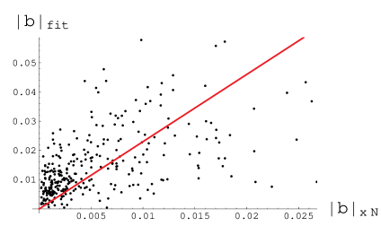
Figure 13: A plot of the sextupole Poisson noise estimate (horizontal axis) versus the magnitude of the sextupole coefficient. The galaxies falling below the straight line with slope 2.3 will be cut as having signal-to-noise ratios too small.

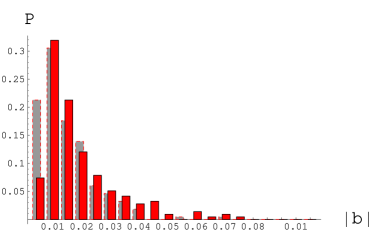
Figure 14: Comparison, after signal-to-noise cut, of the magnitude of the sextupole map coefficients for the moment method (background) and the radial fit method (foreground) (left plot) and of their angular orientation (right plot).

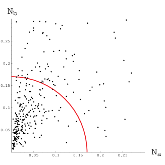
Figure 15: A plot of the ratio $N_{a}=\frac{1}{2}\left[\tan^{-1}|\frac{a_{x\,N}}{a_{fit}}|\right]$ versus the ratio $N_{b}=\frac{1}{3}\left[\tan^{-1}\big{|}\frac{b_{x\,N}}{b_{fit}}\big{|}\right]$. The circle shows the “cut” condition of eq. 40. The galaxies falling outside the circle will be cut as having the quadratically-combined signal-to-noise ratios too small.

Finally, fig. 15 addresses the combination of resolutions that can be expected for $a$ and $b$, showing the condition formulated above in eq. 40. It is this cut that we will impose when we consider the relative orientation of the quadrupole and sextupole map coefficients. 217 galaxies survive this cut.

The following list summarizes the results on the several galaxy cuts. If a line is indented with respect to a line above it, then the cut is for the combination of these conditions.

569     in the z-catalog with $z>0.8$ and found by SExtractor for thresholds 4$\sigma_{NF}$ and 6$\sigma_{NF}$

427     having only one prominent maximum

370     larger than 5 pixels in both x and y

323     with radial-fit having its L2 squared norm less than 0.05

276     with quadrupole signal/noise greater than 4.5

216     with sextupole signal/noise greater than 2.3

217     satisfying the joint-variable signal-to-noise cut condition of eq. 40

Only a very few galaxies had $|a|+2|b|r_{Max}>1$, so this cut was not enforced. Further signal-to-noise cuts, arising for the $c$ and $d$ terms, must be combined with the above cuts to establish their orientation with respect to the imputed direction to the scattering center. Since these cause the surviving statistical sample to become uncomfortably small, we will postpone a discussion of the relevance of the $c$ and $d$ terms, if any, to a subsequent paper with larger statistical samples.

6.3 Sextupole coefficients from model method

The distribution of the sextupole-coefficient magnitudes for the model method is shown in fig. 16 (left plot), and the comparison of the orientation of the sextupole coefficient orientation for the model and radial-fit method are shown in fig. 16 (right plot). The relevant difference in sextupole angle, as noted above, is $30^{\circ}$. Many galaxies have changed by that amount, indicating the importance of the PSF correction.

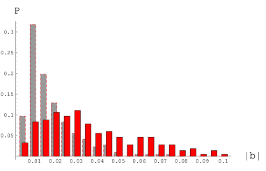
Figure 16: The left panel shows the distribution of the magnitude of the sextupole map coefficient, for the model method (foreground) as compared with the radial-fit method (background). The units are ”per HDF pixel”. The right panel compares the angular orientation of the sextupole map coefficient for the model method and the radial fit method.

Fig. 17 (left) shows the distribution of sextupole coefficients that were found by computing moments of the PSF after it had been dithered, diffused and drizzled. The right panel shows the orientation of the sextupole moment, with the lines of each symbol pointing toward the three sextupole shape maximum. Remarkably, the sextupole-moment orientation is uniform across each chip. This may be helpful in following time variation of the sextupole coefficient, if any is present.

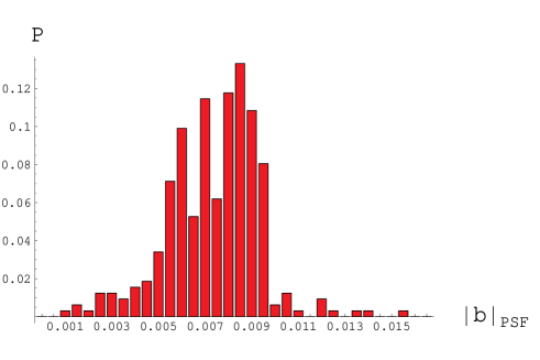
Figure 17: Spatial distribution of sextupole orientations (left) and the sextupole coefficient distribution (right) for the 5x subsampled and drizzled Tiny Tim PSFs for the WPFC2 camera on the Hubble.

6.4 Relative orientation of the quadrupole and sextupole map coefficients

The orientation of the sextupole map coefficient with respect to the quadrupole coefficient is of primary interest to us. A plot of the (smallest) angle between sextupole and quadrupole minima using the model method is shown in fig. 18 for the galaxies surviving both the L2 norm $<$ 0.05 cut and the signal-to-noise cut of eq. 40. This angle, which we refer to as $\delta$, runs from $0^{\circ}$ to $30^{\circ}$. For $\delta=30^{\circ}$ the shapes will have aligned maxima, and we refer to such galaxies as “aligned”. They are pear shaped galaxies, as compared to the “curved” galaxies which resemble bananas. See fig. 1.

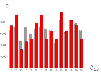
Figure 18: The distribuiton of the magnitude of $\delta$, the smallest angle between a quadrupole minimum and a sextupole minimum, using the model method, for galaxies in the north HDF surviving the cut condition of eq. 40 (foreground) and all galaxies surviving the L2 cut (background).

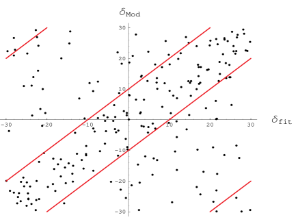
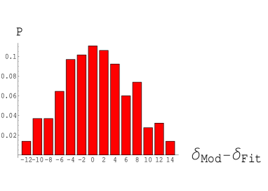
Figure 19: The left panel compares the angle $\delta$ as measured by the radial-fit method and the model method. The points within the diagonal band (or in the corners) have a change in $\delta<10^{\circ}$ . The distribution for $\delta_{Mod}-\delta_{Fit}$ is shown on the right panel.

Figure 19 compares $\delta$ found with the radial-fit and model methods. About one-third of all galaxies show a change in $\delta$ or greater than $10^{\circ}$. This is a concern because it means that the point-spread function does indeed play an important role in distinguishing “curved” from “non-curved” galaxies. This would not be as great a concern if the PSF was well known, but unfortunately the PSF is known to vary with time. We will return to a discussion of the role of the PSF in subsection 9.2.

We now proceed to a study of the spatial distributions of the “curved” and “aligned” galaxies as determined in this section.

7 Clumping probabilities

To quantify clumping for a particular galaxy subset with ${\it N}$ (e.g. the number of curved) members, we draw a circle of fixed radius $R$ about each member of the subset and count the members of that subset which lie within the circle. We then compare the distribution of the number of galaxies having the number of neighbors $N\,=\,0,\,1,\,2,\,3,$ etc. within the circle, with a large number of such distributions derived from randomly chosen subsets having the same number (${\it N}$) of galaxies in two distinct ways:

1. for an informative but qualitative comparison, we compare the distribution of the particular subset with the average distribution of the random subsets, and

2. for a quantitative comparison, for the particular subset being studied and for each of 500 randomly selected subsets having the same number of galaxies as the original subset, we sum the galaxies having $N\geq N_{Min}$ or more neighbors (usually $3\leq N_{Min}\leq 7$). Each random subset is thereby associated with a single number, $n_{G}$, the number of galaxies of that subset having $N_{Min}$ or more neighbors. We then create a bar graph, showing for each value for $n_{G}$ the number of random subsets which had $n_{G}$ galaxies with $N_{Min}$ or more neighbors. This distribution is thus a property of random subsets with ${\it N}$ members, with specified neighbor distance $R$, for the specified neighbor range ($N\geq N_{Min}$). Since the initial subset will have a certain number, $n_{G0}$, of galaxies having $N_{Min}$ or more neighbors, we can ask the question “what fraction of randomly chosen galaxy subsets have $n_{G0}$ or more galaxies with $N_{Min}$ or more neighbors?” We thereby determine a probability that this configuration could occur by chance.

In a variation of this, the randomly chosen subsets, may be constrained in some way. For example, we may wish to look only at randomly chosen subsets whose members are selected to have the same z-distribution as the galaxies in the original set.

In this section we will show examples of: a) bar graphs showing the galaxy fraction ($P$) versus number of neighbors, for both the observed subset and for the average of 500 random subsets, whether the observed subset be “aligned”, “mid-range”, or “curved”; b) bar graphs showing the number of galaxies having $N$ or more neighbors for 500 random subsets of the background galaxies (after cuts); and c)field plots showing the spatial location in the field of the “curved” galaxies and the “aligned” galaxies. On these field plots may also be shown: i) all background galaxies after cuts, ii) the direction of the curvature of “curved” galaxies, iii) the orientation of the “aligned” galaxies, iv) the circular areas defining the neighbors of each “curved” or “aligned” galaxies, v) the combined circular areas of distinct groups, vi) the z-values of the‘ ‘curved” or “aligned” galaxies, or viii) some combination of these.

7.1 “Curved” galaxies

For “curved” galaxies we begin with bar graphs of type $1$. In fig. 20 (a), we show the distribution of the number of neighbors in a circle of radius $R=280$ for the “curved” galaxies using the radial-fit method (which we now take to be $\delta<9^{\circ}$.) In fig. 20(b) we show the same distribution using the model method.

    

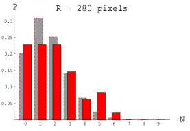
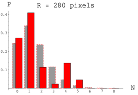
  (a)   “Radial-fit”                                    (b)   “Model”

Figure 20: For two methods, a histogram showing the fraction of curved galaxies having a specific number, N, of curved neighbors within a circle of radius 280 pixels, compared with the average of such a distribution for 500 randomly chosen subsets having the same number of galaxies.

In fig. 21 we show for the model method how this distribution changes as the radius of the circle is varied.

     

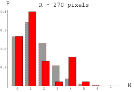
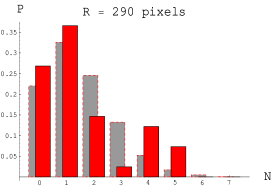
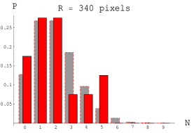
Figure 21: The same “neighbors” histogram for curved galaxies in the north HDF in the circle with R = 270, 290 and 340 pixels, using the model method.

  

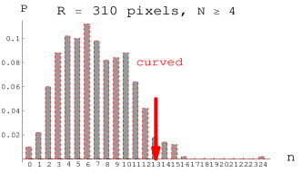
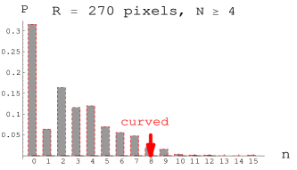
   (a)   “Radial-fit”                           (b)   “Model”

Figure 22: Histogram of numbers of galaxies in 500 randomly chosen sets having 4 or more neighbors in the circles of 310 and 270 pixels. The red arrow indicates the number of “curved” galaxies with N or more neighbors for the “curved” set.

Fig. 22(a) displays an analysis of type $2$ for the radial-fit method. (The number $n_{G0}$corresponding to the “curved” set is indicated by an arrow in this bar graph.) For the optimum radius, of 310 pixels, there will be 21 out of 500 sets that have as many galaxy-circles with counts equal to or greater than the original curved set. In other words, the probability of achieving the curved set by chance is equal to or smaller than 4%. Fig. 22(b) displays an analysis of the type $2$ for the model method. The optimum radius is now 270 pixels, and the probability to achieve the curved set by chance is equal to or smaller than $4\%$.

  

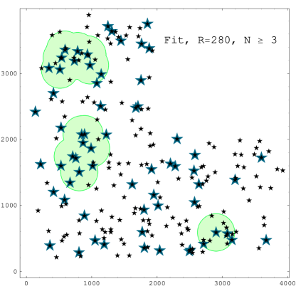
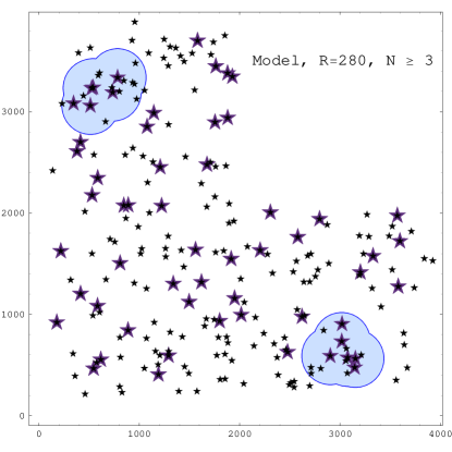
Figure 23: A field plot showing the spatial location of “curved” galaxies in the north HDF using the radial-fit (left panel) and model (right panel) methods to determine the map coefficients. Large “stars” indicate “curved” galaxies and small “stars” indicate the remaining background galaxies that survived the joint-variable signal-to-noise cut. Circles are shown for 3 or more neighbors.

We now turn to the field plots. Figure 23 shows “curved” galaxies in the Hubble north field and for galaxies having three or more neighbors, their neighborhood circles of radius R=280 pixels. Panel (a) shows clumping of “curved” galaxies as determined using the radial-fit method. This can be compared with (b) the same plot with “curved” as determined using model method. In these plots, large “stars” indicate “curved” galaxies, and small “stars” indicate remaining background galaxies.

As seen in fig. 18 the change in $\delta$ is large enough so that many galaxies would move across the boundary defining “curved” galaxies. Still, the overall pattern remains remarkably similar for the two methods.

  

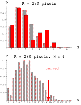
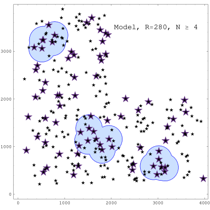
Figure 24: A “neighbors” histogram and a field plot showing the spatial location of “curved” galaxies in the north HDF using the model method to determine the map coefficients. Circles are shown for 4 or more neighbors.

Next we carry through the same analysis for a less stringent noise cut. See figures 24 a-c. Remarkably the probability to randomly achieve the resultant clumping decreases to $3\%$ for the model method as we increase the radius of the noise cut condition of eq. 40 from 0.17 to 0.25. For an orientation to this cut change, see fig. 15. If we were truly adding noise, one would expect the distribution to become more random, not less. The new field plot is shown in fig. 24 c. There is now a $3^{rd}$ major clump.

Finally we note that the random conditions often include rather improbable z-distributions. If we require the randomly chosen galaxy subsets to have z-distributions approximating the actual z-distribution, the probability decreases from $3\%$ to $1\%$.

7.2 “Aligned” galaxies

Dark matter clusters with haloes in the sextupole lensing mass range will statistically move the observed shapes of background galaxies to a “more curved” condition. See sections 8.3 and 8.4. The regions of the field occupied by haloes slightly enhance the number of curved galaxies and deplete the number of aligned galaxies. For this reason we now apply our analysis of “curved” galaxies to “aligned galaxies”.

In fig. 25(a)we show an example of type $1$. The distribution shows the number of “aligned” galaxies in a circle of radius $R=350$ using the radial-fit method (which we take to be $\delta>20^{\circ}$.) In fig. 25(b) we show the same distribution using the model method.

    

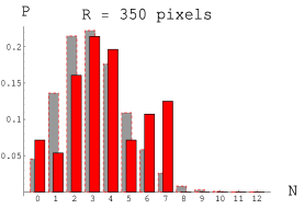
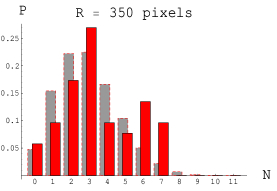
         (a)   “Radial-fit”                           (b)   “Model”

Figure 25: Histograms show the distribution of the number of “aligned” neighbors of “aligned” galaxies within a circle of radius 350 pixels, compared with the average of such a distribution for 500 randomly chosen subsets of galaxies in the north HDF having the same number of members.

In fig. 26 we show what happens as the radius of the circle is varied, using the model method (which is typical of the other methods).

     

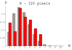
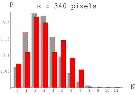
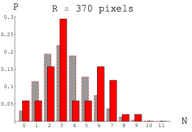
Figure 26: A “neighbors” histogram for “aligned” galaxies as defined using the model method for the north HDF North in circle of radius a) R = 320, b) 340 and c) 370 pixels, respectively.

Fig. 27(a, b) displays an analysis of the type $2$ for the radial-fit and model methods. Typically, for the optimum radius, which is usually 350-370 pixels, there will be less than 25 out of 500 sets that have as many galaxy-circles with counts equal to or greater than the original curved set. In other words, the probability of achieving the “aligned” set by chance is equal to or smaller than 4%.

    

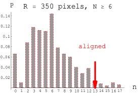
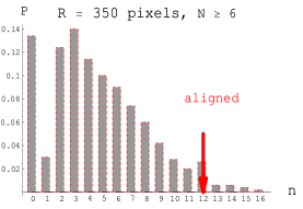
         (a)   “Radial-fit”                           (b)   “Model”

Figure 27: Histogram of numbers of galaxies in 500 randomly chosen sets having 6 or more neighbors in a circle of 340 pixels. The red arrow indicates the number of “aligned” galaxies with 6 or more neighbors for the “aligned” set.

Finally fig. 28(a) shows “aligned” galaxies in the Hubble north field and their neighborhood circles of radius R=350 pixels, using the radial-fit method. This can be compared with (b) the same plot using model method. In these plots, large “stars” indicate “aligned” galaxies and small “stars” indicate background galaxies. Shaded areas show the combined interiors of the “aligned” neighborhood circles.

  

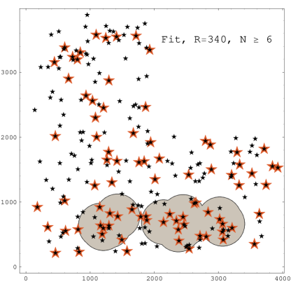
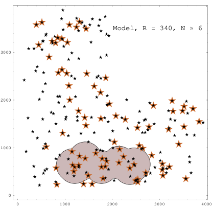
Figure 28: “Aligned” galaxies in the north HDF field comparing radial-fit and model methods to determine the map coefficients. Neighborhood circles have a radius of 340 pixels, and must contain 4 or more neighbors. The left panel used the model method and right panel used the radial-fit method. Green shaded areas show the combined interiors of the “aligned” neighborhood circles.

That aligned galaxies are also clumped is not a trivial consequence of the fact that curved galaxies are clumped. Indeed galaxies midway between curved and aligned are not clumped. And though the aligned set is not completely independent of the curved set (it represents $\raise 2.15277pt\hbox{$\scriptstyle 1$}\kern-1.00006pt/\kern-1.49994pt\lower 1.07639pt\hbox{$\scriptstyle 2$}$ of the complement of the curved galaxies), we maintain that it is independent enough to assert that the probability of finding both of these sets to be clumped by chance is the product of the probability of each.

7.3 “Mid-range” galaxies

    

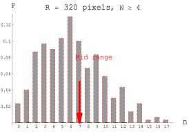
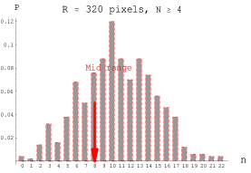
         (a)   “Radial-fit”                           (b)   “Model”

Figure 29: Histogram of numbers of galaxies in 300 randomly chosen sets having 4 or more neighbors in a circle of 320 pixels. The red arrow indicates the number of “mid-range” galaxies with 4 or more neighbors.

A look at mid-range galaxies shows they are behaving quite differently. Fig. 29 displays an analysis of the type $2$ for (a) the radial-fit method, and (b) the model method. (The number corresponding to the “mid-range” set is indicated by an arrow in this bar graph.) There is no indication of the presence of clumping.

8 Dark matter sextupole lensing?

The previous sections have outlined a theory for sextupole lensing and described map coefficient measurements and the search for correlations among coefficient orientation present in the north Hubble deep field. This section inquires whether those observations can be explained by the concordance $\Lambda CDM$ model.

The first subsection discusses the mass and impact parameter requirements of the constituent lens halo. The second subsection makes an analytical estimate of the total lensing mass required, and describes simple simulations supporting this estimate.

The third subsection uses standard $\Lambda CDM$ to compute the halo mass distribution in the Hubble foreground, showing for example that $80\%$ of the range should be visible.

The fourth subsection finds that based on the observed over- and underdensities of foreground visible galaxies, the imputed dark matter overdensities are adequate to account for the clumping signal observed.

Finally in the fourth subsection we compare the location of the over- and underdensities with the location of the curved galaxy clumps.

8.1 Mass range of lensing haloes

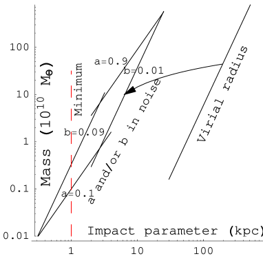
Figure 30: A plot of the constituent lensing mass versus the impact parameter for a lensing plane at $z=0.6$. Lines of constant $a$ and $b$ delineate the lensing envelope required to compete with the range of background values observed with the model method. The angular size of background galaxies establishes the minimum possible impact parameter. In the standard $\Lambda CDM$ the virial radius goes as $M^{1/3}$. This establishes a line on which dark matter haloes reside. The induced map parameters $a$ and $b$ for light streams that penetrate this halo will fall along curved lines. An example of such a curve is shown.

In order to establish correlations in the quadrupole and sextupole map-coefficient alignment, lensing-induced coefficients must be competitive with background values, hence at least comparable with or larger than the minimum observed background values. This simple fact creates limits on the range of acceptable lensing mass and impact parameters.

Fig. 30 shows a plot of mass $M$ and impact parameter $r_{0}$ for lensing haloes located at $z=0.6$ for $D_{LS}=D_{LT}$. The situation on this lensing plane is typical. Constant values of $a$ and $b$ from lensing are straight lines on this log-log diagram with slopes of 2 and 3 respectively. For example, quadrupole coefficients less than 0.1 or sextupole coefficients smaller than 0.01 would not be observable because they would be lost in the noise.

Impact parameters smaller than about 1 kpc are excluded because the radius of the background-galaxy light-path footprints are at least 2.5 pixels, which is about 0.7 kpc on the $z=0.6$ plane. This minimum impact parameter is shown in fig.30.

According to the concordance model the outer radius of dark matter haloes, referred to as the virial radius, $r_{V}$, depends on the total (virial) mass simply as $r_{V}\,\varpropto\,{M_{V}}^{1/3}$. The constant of proportionality may be established by taking $r_{V}=300$ kpc for $M_{V}=1.6\;10^{12}M_{\odot}$. Thus the locus of dark matter haloes is the straight line indicated in fig.30. The $a$ and $b$ induced in a light stream at the virial radius is far too small to be of interest.

However these halo radii are large and light streams will surely traverse their interiors. Using a standard NFW profile (Navarro et. al., 1996) one can integrate out the longitudinal variable perpendicular to the lensing plane and calculate the induced $a$ and $b$ within the interior of the integrated mass distribution. The result is quite simple, namely $a$ and $b$ are given to good accuracy by constants times $M(r)/r^{2}$ and $M(r)/r^{3}$, respectively. This is true because of the radial logarithmic behavior of the integrated interior mass. Thus we can follow the behavior of $a$ and $b$ by following the interior mass vs. radius. An example curve is shown in fig.30.

One finds that the observable lensing region is entered just about when the radius reaches the so-called “scale” radius, the radius at which the profile shifts from logarithmic. In other words, our finding is that the cores of dark matter haloes are dense enough to cause sextupole lensing, and this is true for all haloes with mass greater than about $5\,10^{9}M_{\odot}$ up to a mass of $2\,10^{13}M_{\odot}$.

8.2 Required lensing mass overdensities

We continue to assume the lensing mass lies on the z=0.6 plane. We emphasize that any mass in the foreground field could be projected onto this plane if the lensing mass is modified to compensate for the change in the lever arm coefficient.

Let us assume for simplicity that we are dealing with a single constituent with a lensing mass of $10^{10}M_{\odot}$, and that its spatial distribution is approximately a top-hat. These assumptions can easily be lifted and generalized in simulations. According to the considerations of the previous section the radius of such a lens can be no larger than 7 kpc and should be more like 6 kpc.

Because of the paucity of background galaxies, the probability to have a scattering event must be large where clumping is seen. For example, an area of $\pi 280^{2}$ pixels would typically contain 9 to 10 background galaxies. Assuming these are equally divided between curved, mid-range and aligned, then of the 6 non-curved background galaxies, to achieve a total of 5 curved at least 2 must get curved by lensing. So the probability for a background galaxy to be lensed by a sufficiently small impact parameter must be the order of $33\%$.

We can factor the probability to be transformed from not-curved to curved into a probability that the background galaxy is suitable (the background coefficient is small enough to easily alter and/or its orientation is conducive to change) times the probability that the lensing kick is large enough. If we assume that these probabilities are about equal, then each of these probabilities must be near $60\%$. This probability will be the fractional area occupied by lenses which produce lensing. In other words we have to occupy a hefty $60\%$ of the field with haloes capable of lensing “suitable” background galaxies.

Taking the radius of the lens to be 5 kpc, then to achieve $60\%$ we need $0.6(75/3)^{2}=375$ lenses, or in other words a lensing mass totaling $4\;10^{12}M_{\odot}$. This translates to a total virial mass of $1.8\,10^{13}M_{\odot}$.

To check this estimate we constructed two simulations. One simulation placed 300 lensing masses of $1.5\,10^{10}M_{\odot}$ randomly in a circle of radius 280 pixels at $z=0.6$. 1000 light-paths were randomly chosen through this lens and the lensing coefficients were calculated for each path. Then random background noise values of the map coefficients, based on the measured values, were added to the lensing coefficients for each path. Finally 1000 subsets of these 1000 light paths were randomly selected. The number of paths in each subset was randomized based on a Poisson distribution with a mean equal to the average density of galaxies in the field. For each subset the number of curved and aligned galaxies were determined. Then subsets with 9 or more members were selected. Of these subsets $50\%$ had 5 or more curved galaxies as compared to $20\%$ if the lensing mass was set to zero. In other words, a lens with a total mass of $4.5\,10^{12}\,M_{\odot}$ dramatically increases the probability of finding 5 or more curved galaxies when there are 9 or more background galaxies in the lens area. This result was verified to hold as well for the range of other constituent mass values.

A second simulation actually placed lenses of radius 280 pixels within the field, and circles were used to identify clumping, as in section 7. Analagous results on lens requirements were obtained.

The bottom line of our simple simulations and analytical estimate is that a lensing mass in the range of $5\,10^{12}\,M_{\odot}$ is both necessary and sufficient to produce the observed clumping of curved galaxies. Since aligned galaxies are depleted in these simulations, they support clumping of aligned galaxies as well.

8.3 Mass in the Hubble deep field foreground

In fig. 31 we have plotted the geometric lever-arm coefficients (the product of the $D$’s in eq.7) for the quadrupole and sextupole map coefficients for a “median z=1.64” background galaxy.

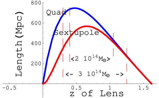
Figure 31: A plot of the lever arm coefficients as a function of the position of the lensing plane for the quadrupole and sextupole map coefficients for the median $z=1.64$ background galaxy. These coefficients are given by $D_{LS}\frac{D_{TL}}{D_{TS}}$ and $D_{LS}\left({\frac{D_{TL}}{D_{TS}}}\right)^{2}$ respectively. The original mass residing in the regions of large lever-arm and small lever-arm coefficient are indicated.

The geometric coefficients are large for the range $0.3<z<1.25$, and hence dark matter haloes in this z-region could give rise to lensing. We will refer to this region as the foreground. The co-moving volume is a needle-like truncated pyramid, having an angular width of only 0.75 milliradian. The co-moving distance to z=1.25 is 3.9 Gpc, and to z=0.3 is 1.2 Gpc. The co-moving volume “behind” the 3 WFPC chips between z=0.3 and z=1.25 is about $8000\,Mpc^{3}$. Using a matter density of 0.27 times the critical density ($3.7\,10^{10}\frac{M_{\odot}}{Mpc^{3}}$) for the original mass density, would imply that this volume originally contained a dark plus baryonic mass of $3\,10^{14}M_{\odot}$.

To get an estimate for the number of haloes within the acceptable mass range as determined in the previous subsection, one can use the Sheth-Tormen distribution (Sheth and Tormen, 1999), which is supported by N-body simulations (Reed et al., 2003). The result is that about $1.6\,10^{14}M_{\odot}$ lies in the mass range between $7\;10^{9}$ and $2.3\,10^{13}M_{\odot}$, amounting to $40\%$ of the total halo mass.

Breaking down the $1.6\,10^{14}M_{\odot}$ by decade, gives roughly: $6\;10^{13}M_{\odot}$ (9 haloes) between $2.3\,10^{12}$ and $2.3\,10^{13}M_{\odot}$; $4.7\,10^{13}M_{\odot}$ (64 haloes) between $2.3\,10^{11}$ and $2.3\,10^{12}M_{\odot}$; $3.5\,10^{13}M_{\odot}$ (480 haloes) between $2.3\,10^{10}$ and $2.3\,10^{11}M_{\odot}$; and $1.5\,10^{13}M_{\odot}$ (1140 haloes) between $7\,10^{9}$ and $2.3\,10^{10}M_{\odot}$.

A circle of radius 280 pixels represents about $2.2\%$ of the field, hence on the average such a circle has a foreground mass of $3.6\,10^{12}M_{\odot}$. Dividing that mass by 4.5 yields the core mass of these halos, $8\,10^{11}M_{\odot}$. With an overdensity of 3 this would give a core lensing mass of $2.4\,10^{12}M_{\odot}$, pretty close to the required $5\,10^{12}M_{\odot}$.

8.4 Visible foreground galaxy distribution

Dark matter haloes within the top end of the mass range described in section 8.1 should contain visible galaxies. There are 420 observable galaxies in the foreground z-range, indicating haloes down to perhaps $3\,10^{10}M_{\odot}$ are bright enough to be seen. According to the considerations of the previous section this represents $80\%$ of the mass in the range important for sextupole lensing. Hence we can take the visible galaxy overdensities as markers for the invisible dark matter halo overdensities.

In fig. 32(a) we plot the positions of the 420 foreground galaxies on a grid of 192 boxes. The occupancy count varies from 1 to 7, with a mean of 2.17 galaxies per box. Darker boxes indicate larger numbers of foreground galaxies. There are 5 boxes with an overdensity of 3 or more times the average density.

In fig. 32(b) we show the background galaxies on the same grid as fig. 32(a). According to our conjecture, to obtain a clump of curved galaxies one would need to have i) an overdensity of foreground haloes and ii) at least 9 or more background galaxies probing the overdense region. In fig. 32(a) one can identify five regions with large foreground overdensities (excluding border regions). Upon checking out these regions in fig. 32(b) one sees that two of those five do not have the prerequisite number of background galaxies probing the region. The three curved clumps of fig. 24 intersect the remaining three regions. This does not prove our conjecture, but is certainly estalishes that a lensing scenario is consistent with our observations and $\Lambda CDM$.

  

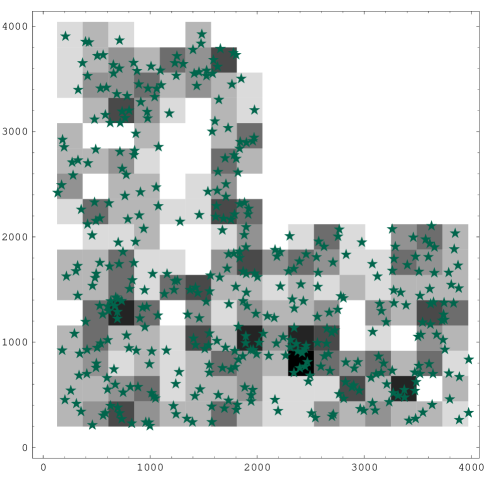
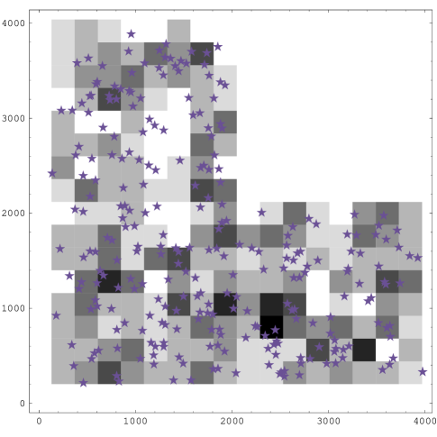
(a)                                                                        (b)

Figure 32: In the left panel foreground galaxies are shown as (dark green) stars on a grid of 192 square boxes. The boxes are shaded according to galaxy density, black being the most dense areas. In the right panel we show the same grid with the background galaxies shown as (dark blue) stars.

9 Systematic error sources

In this section we turn our attention to possible systematic non-lensing sources of the observed clumping.

9.1 Background galaxy clumping

Could the observed clumping of curved galaxies originate in the background galaxies themselves? Since the galaxies at any given slice in $z$ are known to be spatially correlated, clumping would naturally result if the galaxies in particular galaxy-groups possessed the features we are measuring. This could arise in two distinct ways: i) there might be some age-dependent process at work. For example, perhaps old galaxies are more curved. Or ii) perhaps some galaxy groups tend to be more curved than others, because of some common history or composition.

In response to item i) one can look at the z-distribution of “curved” or “aligned” galaxies to see if there is any evidence of a bias in the population. Figure 33 compares the z-distribution of “curved” galaxies with all galaxies. and the z-distribution of “aligned” galaxies with all galaxies. There is no particular evidence that older galaxies are more or less curved or aligned, according to our criteria for curved and aligned.

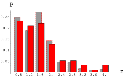
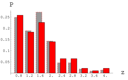
Figure 33: The left bar graph compares the z-distribution of “curved” galaxies in the foreground bars and all galaxies in the background bars. The right bar graph compares the z-distribution of “aligned” galaxies in the foreground bars and all galaxies in the background bars.).

To address item ii) we first note that z-values are measured in intervals of $\Delta z=0.02$. At $z=1.0,\,2.0,\mbox{ and }3.0$, a separation of $\Delta z=0.02$ corresponds to a co-moving separation of $50,\,30,\,\mbox{ and }\,20\,Mpc$, respectively. Therefore, galaxies in different z-bins are well-separated in 3-dimensional space, and an event in one group should not be able to influence another group. Hence item ii) also appears unlikely, for 3 reasons:

1. None of the z-bin groups seems to be especially curved. Plotting fig. 33 for $\Delta z=0.02$ bins, shows no striking evidence that any group is particularly curved.

2. Same z-bin galaxy groups are spread across large regions of the Hubble field. Their inter-galaxy separation is typically larger than the scale of the correlation we are noticing.

3. For each actual “curved” group we have observed, all members have distinct z-values. Therefore their curvature could not arise from a single causative event. This can be see in the left panel of fig. 34, where the z-values are printed alongside the curved galaxies. One can check the groups to verify that in each group there is no z-value occurring more than one time. The z-values for the upper left “curved” clump are $z=1.12,\,1.16,\,1.56,\,1.72,\,2.12,\mbox{ and }3.00.$ The z-values for the lower right “curved” clump are $z=0.08,\,1.64,\,1.72,\,2.16,\,2.24,\mbox{ and }3.10.$

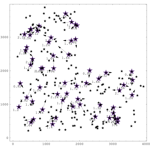
Figure 34: Curved galaxies in the north HDF using the model methods to determine the map coefficients: arrows for each curved galaxy point to the center of curvature and the z-values of the “curved” galaxies are indicated.

In summary, we find it to be highly unlikely that the excess clumping we are seeing for both “curved” and “aligned” galaxies could result from correlated shapes present in the background galaxies themselves.

9.2 PSF residuals

We know that the PSF correction plays a role in the determination of which galaxies are “curved” and we have made an effort to remove the PSF effects, but are there significant residuals? Unfortunately the PSF can vary with time, as the temperature of the Hubble telescope changes. However there are reasons to doubt the observed clumping is coming from the PSF.

Figures 11 and 17 show the orientation and magnitude of the quadrupole and sextupole coefficient for the Tiny Tim PSF, respectively. We note that the orientation of the sextupole coefficient is almost constant in each chip and the magnitude varies only slightly. This is in strong contrast to the quadrupole moment which gets stronger at the edge of the chips and whose orientation follows large circles, centered roughly on the chip. Combining these two would result in a pattern that would repeat six times around each circle (curved $\rightarrow$ mid-range $\rightarrow$ aligned $\rightarrow$ mid-range $\rightarrow$ curved $\rightarrow$ …). For 3 orientations of the quadrupole a minimum is aligned with a minimum of the sextupole, and each such orientation occurs twice, on opposite sides of the circle. The radius of this circle is $\sim 800$ pixels, hence the circumference is $\sim 4800$ pixels. Each repeat has a length of $\sim 800$ pixels, hence the curved region width would be $\sim 270$ pixels. In other words these regions would have half the radius of the clumped regions we have found, and one-quarter the area.

No such pattern is apparent, and the regions predicted to be curved do not correspond to the location of our clumped regions. Since the PSF “curvature” would vary continuously across the field, galaxies within one of the curved regions would all curve the same way, curving galaxies the same way within each clump. Furthermore there is no evidence of the uni-directional curving that would be predicted. See fig. 34.

The time-variation is thought to change the quadrupole strength, but not flip its direction. Therefore, even in the case of time variation, the pattern could be expected to follow the description of the preceding paragraph.

9.3 Image composition

Since we suspect we are processing images in a way not originally anticipated by the creators of the image composition process, we were concerned that our observations could be due to a feature of that process. We raised this concern with the Space Telescope Science Institute, who assured us that: “To (our) knowledge, there are no instrument artifacts or any portion of the image processing and stacking which would mimic the curvature you are noting in the background galaxies.”

The final image is the co-addition and “drizzling” of images that were taken with nine distinctly “dithered” pointings, enabling the resolution of the composite image to be higher than any single image. The dither offsets have to be known accurately at each point on the focal plane, or else the co-addition will indeed yield image moments not present in the original images. But this is a question of magnitude. As we have repeatedly pointed out, the magnitude of any distortion must be the order of the observed moments themselves. In the case of the quadrupole, suppose we have a false separation of two symmetrical images each offset by $\Delta$ but in opposite directions. Then a false quadrupole map coefficient of magnitude $1/2(\Delta/r_{0})^{2}$ will be generated. For this to have a magnitude of a typical $a\approx 0.2$ would require $\Delta/r_{0}\sim 0.6$. Since our typical $r_{0}\geq 3$ , this would require $\Delta\geq 1.8$ HDF pixels. In our opinion, this is an improbably large offset. We would estimate false offsets to be at most 1/4 this size (0.2 original camera pixels). With the effect going as the square that would be a factor of 16 too small. Similarly the false sextupole generated by three images each offset in a triangular configuration by $\Delta$ would have a sextupole coefficient of magnitude $1/6(\Delta^{3}/r_{0}^{4})$. For this to have a magnitude of 0.02 even for $r_{0}=3$ would require $\Delta\geq 2$ HDF pixels, again at least 4x larger than expected false offsets.

If there were errors in the dither amplitudes, one would expect these errors to be coherent across the field, that is all of the galaxies in a local region would have the same errors in the co-addition process. This would result in a spatial clumping of curvature, but all the galaxies in any given local region would appear to be curved in the same direction. This is not what we see.

We also note that the regions where curved galaxies clump do not appear to have any particular identifiable pattern, i.e. they do not appear to coincide with chip boundaries.

9.4 Pixel-derived effects

Early on we had a concern that spurious sextupole moments could be generated by the simple process of pixelating an image. To probe this, we took known typically sized bi-Gaussian distributions and, varying the centroid, dropped them onto a pixel grid. To our surprise, the falsely induced sextupole map coefficients had strengths less than $10^{-5}$. Square pixel grids do give rise to spurious octupole moments, and sensitivity limits are set in that case.

Of course pixel defects will give rise to spurious changes in galaxy shapes. By taking a hole out of one side of an image, a spurious curvature would be induced. Defects in the quantity and arrangement required would seem like a serious camera defect.

9.5 Galaxy selection effects

Galaxy selection software would appear to be blind to position in space and incapable of leading to the spatial clumping of curved or aligned galaxies

10 Summary

We visually examined galaxy images selected by the SExtractor software from the Hubble deep fields. After filtering images with two or more major maxima, we imputed sextupole and quadrupole map coefficient strengths using a moment method, a radial-fit method and a model method. The model method includes convolution with the PSF of the Hubble, charge diffusion and an emulation of the dither and drizzle process. The “curved” galaxies we sought were identified as those whose sextupole coefficient was oriented with one of its minima within $10^{\circ}$ of a quadrupole minima. The “aligned” galaxies have maxima aligned within $10^{\circ}$. We then looked for and found a spatial clumping in the Hubble deep field of “curved” and “aligned” galaxies. The probability of “curved” clumping to occur by chance was found to be about 1% for a weak noise cut and constrained z-distributions on randomly selected galaxy subsets. The probability of “aligned” clumping to occur by chance was found to be about 4%.

Our lensing hypothesis proposes that within the observed clumps of curved background galaxies a couple images are curved by close collisions with dark matter haloes residing in the field foreground. Simulations and analytical estimates indicate the required total lensing mass $\sim 5\,10^{12}M_{\odot}$. Such a mass is similar to the total mass expected in overdensities of the foreground dark matter halo cores. Furthermore there appears to be a correlation between foreground galaxy overdensities and the observed curved clumps.

Unfortunately the quadrupole moment of the PSF is known to vary with time and temperature. We are hesitant to claim an observation of small scale structure without a better characterization of the PSF and without better statistics. Fortunately the Hubble ACS camera is providing larger fields, and efforts are underway to characterize the time dependence of it’s PSF. .

The Hubble deep fields are less than 2 min by 2 min, $\sim 10^{-3}$ sq. deg. A space-based project in the planning stages (the SuperNova /Acceleration Probe (SNAP) (Aldering et al., 2002; Rhodes et al., 2003; Massey et al., 2003; Refregier et al., 2003)) has a weak lensing program of $\sim$ 1000 sq. degrees ($10^{6}$ times the Hubble deep field) with comparable resolution, better characterization of the PSF, and deep enough to provide $\sim 100$ background galaxy images per sq. min.

Acknowledgements

We would like to acknowledge the encouragement and support of Tony Tyson and David Wittman of Bell Labs. Visits by both of us to Bell-Labs prepared us for this undertaking, especially introducing us to existing software and weak-lensing techniques. We would also like to thank Pisin Chen and Ron Ruth at SLAC for trusting in our judgment and encouraging us to proceed. This work was supported by DOE grant DE-AC03-76SF00515.

After presenting our ideas to Tony Tyson in January 2002, he suggested we look at a posting by D.M. Goldberg and P. Natarajan titled, “The Galaxy Octupole Moment as a Probe of Weak Lensing Shear Fields” (Goldberg, and Natarajan, 2001). The mathematical formulae presented there were actually what we have been calling the sextupole. Our nomenclature derives from beam physics, where the sextupole field is created by a magnet with six poles, 3 of positive polarity and 3 of negative polarity. To our knowledge, there was no mention by Goldberg and Natarajan of the induced ”sextupole/octupole” shape or using its correlation with the quadrupole shape to distinguish galaxies.

We thank Ken Shen for his assistance in providing a program to identify double-maximum galaxies, and Konstantin Shmakov for help with software.

The first version of this present work was posted in August 2003. (Irwin and Shmakova, 2003b).

Appendix

Imagine that we are considering a background galaxy (S) that has not yet been lensed, and suppose the radial-fit method is used to find $a=a_{S}$. One can imagine a radially symmetric root-galaxy (R) that had a zero $a$ parameter mapped to match the radial behavior and the quadrupole coefficient of background galaxy (S). The corresponding map would be $w_{R}=w_{S}+a_{S}\bar{w}_{S}$.

Now suppose that there is a lensing event described by $w_{S}=w_{T}+a_{L}\bar{w}_{T}.$ The composition of these 2 maps gives

$$w_{R}=(1+\bar{a}_{L}a_{S})w_{T}+(a_{L}+a_{S})\bar{w}_{T}.$$ (41)

The map from the telescope observation (T) to the root-galaxy (R) has $a=a_{L}+a_{S}$. In addition there is a slight rotation and scale change represented by the coefficient of $w_{T}$. Since our measured estimates are based on a unit coefficient for the $w_{T}$ coefficient, we must remove this implicit (undetectable) scaling and rotation. Define a Q (quelle) galaxy that is a scaled root galaxy by $w_{Q}=(1+\bar{a}_{L}a_{S})^{-1}w_{R}.$ Then we have

$$w_{Q}=w_{T}+(1+\bar{a}_{L}a_{S})^{-1}(a_{L}+a_{S})\bar{w}_{T}.$$ (42)

In the case of weak lensing $a_{L}$ is small, so $(1+\bar{a}_{L}a_{S})$ is close to unity and we obtain the simple vector addition $a=a_{L}+a_{S}$. In the case that $a_{L}$ is comparable with $a_{S}$ (say they are both of magnitude 0.4), then the coefficient is still a small adjustment since $|a_{L}a_{S}|\sim 0.16$. The correction is smaller if $a_{L}$ and $a_{S}$ are not aligned. With these parameters the average deviation of $(1+\bar{a}_{L}a_{S})$ from unity is a tiny $1/2|a_{L}a_{S}|^{2}\sim.01$. The bottom line is that the lensing may be added vectorially with the background. The bias error with this approximation can be the order of $1\%$.

To be complete one can carry this through for the sextupole as well. Define

$$w_{R} = w_{S}+a_{S}\bar{w}_{S}+b_{S}{\bar{w}_{S}}^{2}$$ (43)

$$w_{S} = w_{T}+a_{L}\bar{w}_{T}+b_{L}{\bar{w}_{T}}^{2}$$ (44)

yielding

$$w_{R}=(1+\bar{a}_{L}a_{S})w_{T} + (a_{L}+a_{S})\bar{w}_{T}+(b_{L}+b_{S}){\bar{w}_{T}}^{2}$$ (45)

$$+ 2b_{S}\bar{a}_{L}w_{T}\bar{w}_{T}+a_{S}\bar{b}_{L}{w_{T}}^{2}$$ (46)

$$+ b_{S}\bar{b}_{L}\bar{w}_{T}{w_{T}}^{2}+2\bar{a}_{L}b_{S}\bar{b}_{L}{w_{T}}^{3}+b_{S}\bar{b}_{L}{w_{T}}^{4}.$$ (47)

The last line can be dropped as all have products of 2 or more b’s which are the order of $\sim.001$. On the second line we have a new pair of quadratic order terms that we have referred to as d-terms or gradient terms. They will not contribute to the sextupole or quadrupole term. They will be noise in the d-term if that is pursued later. If we had included such terms in the background galaxies these terms could have generated sextupole terms but all would be small since the measured d-terms are typically a factor of 3 smaller than the sextupole terms.

Scaling as before, and dropping the very small terms we get

$$w_{Q}=w_{T}+(1+\bar{a}_{L}a_{S})^{-1}(a_{L}+a_{S})\bar{w}_{T}+(1+\bar{a}_{L}a_{S})^{-1}(b_{L}+b_{S}){\bar{w}_{T}}^{2}+\cdots$$ (48)

The final result is “the measured map coefficient is the simple sum of the lensing coefficient and the background coefficient”, where the background coefficients are those that would have been measured for the galaxy image in the absence of lensing.

References

- Aldering et al. (2002) G. Aldering [the SNAP Collaboration], arXiv:astro-ph/0209550.
- Bartelmann and Schneider (1999) M. Bartelmann and P. Schneider, Phys. Rep. 340 , 291, (2001), arXiv:astro-ph/9912508.
- Bertin and Arnouts (1996) E. Bertin and S. Arnouts, Astron. Astrophys. Suppl. Ser.117, 393 (1996)
- Bond et al. (2002) J. R. Bond et al., “The cosmic microwave background and inflation, then and now,” arXiv:astro-ph/0210007.
- Casertano et al. (2000) S. Casertano et al., arXiv:astro-ph/0010245.
- Davis et al. (1985) M. Davis, G. Efstathiou, C. S. Frenk and S. D. White, Astrophys. J. 292, 371 (1985).
- Goldberg, and Natarajan (2001) D. M. Goldberg, and P. Natarajan, arXiv:astro-ph/0107187
- Hoekstra, Yee, and Gladders (2002) H. Hoekstra, H. Yee and M. Gladders, New Astron. Rev. 46, 767 (2002) [arXiv:astro-ph/0205205].
- Huterer (2001) D. Huterer, Phys. Rev. D 65, 063001 (2002) [arXiv:astro-ph/0106399].
- Huterer and Turner (2000) D. Huterer and M. S. Turner, Phys. Rev. D 64, 123527 (2001) [arXiv:astro-ph/0012510].
- Irwin and Shmakova (2003a) J. Irwin and M. Shmakova, “Cosmological Final Focus Systems”, to be published in the proceedings of 28-th Workshop on “Quantum Aspects of Beam Physics, ” (2003).
- Irwin and Shmakova (2003b) J. Irwin and M. Shmakova, arXiv:astro-ph/0308007.
- Kaiser (2000) N. Kaiser, G. Wilson and G. A. Luppino, arXiv:astro-ph/0003338.
- Kallosh et al. (2003) R. Kallosh, J. Kratochvil, A. Linde, E. V. Linder and M. Shmakova, arXiv:astro-ph/0307185.
- Kallosh and Linde (2003) R. Kallosh and A. Linde, JCAP 0302, 002 (2003) [arXiv:astro-ph/0301087].
- Kuijken (1999) K. Kuijken, “Weak weak lensing: correcting weak shear measurements accurately for PSF anisotropy,” arXiv:astro-ph/9904418.
- Linde (2002) A. Linde, arXiv:hep-th/0211048.
- Linder and Jenkins (2003) E. V. Linder and A. Jenkins, arXiv:astro-ph/0305286.
- Navarro et. al. (1996) J. F. Navarro, C. S. Frenk and S. D. M. White, arXiv:astro-ph/9611107.
- Massey et al. (2003) R. Massey et al., arXiv:astro-ph/0304418;
- Mellier (1998) Y. Mellier, arXiv:astro-ph/9812172.
- Mellier et al. (2002) Y. Mellier, L. van Waerbeke, E. Bertin, I. Tereno and F. Bernardeau, arXiv:astro-ph/0210091.
- Peebles (1994) P. J. Peebles, “Principles Of Physical Cosmology,” Princeton, USA: Univ. Pr. (1994).
- Perlmutter (1999) S. Perlmutter et al., “Measurements of Omega and Lambda from 42 High-Redshift Supernovae,” Astrophys. J. 517, 565 (1999) [astro-ph/9812133], see also http://snap.lbl.gov;
- Reed et al. (2003) D. Reed et al., arXiv:astro-ph/0312544.
- Refregier et al. (2003) A. Refregier et al., arXiv:astro-ph/0304419.
- Rhodes et al. (2003) J. Rhodes, A. Refregier and R. Massey [the SNAP Collaboration], arXiv:astro-ph/0304417;
- Riess et al. (1998) A. G. Riess et al. [Supernova Search Team Collaboration], “Observational Evidence from Supernovae for an Accelerating Universe and a Cosmological Constant,” Astron. J. 116, 1009 (1998) [arXiv:astro-ph/9805201].
- Sheth and Tormen (1999) R. K. Sheth and G. Tormen, Mon. Not. Roy. Astron. Soc. 308, 119 (1999) [arXiv:astro-ph/9901122].
- Sievers et al. (2002) J. L. Sievers et al., “Cosmological Parameters from Cosmic Background Imager Observations and Comparisons with BOOMERANG, DASI, and MAXIMA,” astro-ph/0205387;
- Spergel et al. (2003) D. N. Spergel et al., “First Year Wilkinson Microwave Anisotropy Probe (WMAP) Observations: Determination of Cosmological Parameters,” arXiv:astro-ph/0302209.
- Tegmark and Zaldarriaga (2002) M. Tegmark and M. Zaldarriaga, Phys. Rev. D 66, 103508 (2002) [arXiv:astro-ph/0207047].
- Tonry et al. (2003) J. L. Tonry et al., arXiv:astro-ph/0305008.
- Williams et al. (1996) R. E. Williams [the HDF Team Collaboration], arXiv:astro-ph/9607174.
- Wittman et al. (2000) D. M. Wittman, J. A. Tyson, D. Kirkman, I. Dell’Antonio and G. Bernstein, Nature 405, 143 (2000) [arXiv:astro-ph/0003014].