Type Ia supernovae tests of fractal bubble universe with no cosmic acceleration

Abstract

The unexpected dimness of Type Ia supernovae at redshifts $z\lesssim 1$ has over the past 7 years been seen as an indication that the expansion of the universe is accelerating. A new model cosmology, the “fractal bubble model”, has been proposed by one of us, based on the idea that our observed universe resides in an underdense bubble remnant from a primordial epoch of cosmic inflation, together with a new solution for averaging in an inhomogeneous universe. Although there is no cosmic acceleration, it is claimed that the luminosity distance of type Ia supernovae data will nonetheless fit the new model, since it mimics a Milne universe at low redshifts. In this paper the hypothesis is tested statistically against the available type Ia supernovae data by both chi–square and Bayesian methods. While the standard model with cosmological constant $\Omega_{\Lambda}=1-\Omega_{m}$ is favoured by a Bayesian analysis with wide priors, the comparison depends strongly on the priors chosen for the density parameter, $\Omega_{m}$. The fractal bubble model gives better agreement generally for $\Omega_{m}<0.2$. It also gives reasonably good fits for all the range, $\Omega_{m}=0.01$–$0.55$, allowing the possibility of a viable cosmology with just baryonic matter, or alternatively with both baryonic matter and additional cold dark matter.

1 Introduction

For nearly a decade it has been assumed that the universe is presently undergoing a period of acceleration driven by an exotic form of dark energy. In a new model proposed by one of us (Wiltshire 2005a), it has been claimed that it is possible to fit type Ia supernovae (SNeIa) luminosity distances without exotic forms of dark energy, and without cosmic acceleration. The new model was developed on the basis of a suggestion of Kolb, Matarrese, Notari and Riotto (2005), that cosmological evolution must take into account super–horizon sized remnant perturbations from an epoch of primordial inflation.

The new model cosmology of Wiltshire (2005a,2005b) – henceforth the Fractal Bubble (FB) Model – shares the basic assumption of Kolb et al. (2005) that the observed universe resides within an underdense bubble, SS, in a bulk universe which has the geometry of a spatially flat Friedmann–Robertson–Walker (FRW) geometry on the largest of scales. In other respects, however, the FB model differs substantially from that of Kolb et al. (2005). In particular, the FB model is based on exact solutions of Einstein’s equations, whereas Kolb et al. (2005) based their analysis on linearized perturbations, with a number of approximations. Furthermore, while Kolb et al. suggested that the deceleration parameter would behave as $q(\tau)\to-1$ at late times, in the FB model $q(\tau)\to 0$. The FB model has the added advantage that it can make quantitative predictions for many cosmological quantities in the epoch of matter domination based on two parameters, the Hubble constant, $H_{\lower 2.0pt\hbox{$\scriptstyle 0$}}$, and the density parameter, $\Omega_{m}$.

The FB model makes two crucial physical assumptions. The first, as just mentioned, is that our observed universe resides in an underdense bubble, which is a natural outcome of primordial inflation. The second assumption is that on account of the bottom–up manner in which structure forms and spatial geometry evolves in an inhomogeneous universe with the particular density perturbations that arise from primordial inflation, the local clocks of isotropic observers in average galaxies in bubble walls at the present epoch, are defined in a particular way. The small scale bound systems which correspond to typical stars in typical galaxies retain local geometries with an asymptotic time parameter frozen in to match the cosmic time of the average surfaces of homogeneity in their past light cones at the epoch they broke away from the Hubble flow. That local average geometry was a spatially flat Einstein–de Sitter universe, even though the presently observable universe, SS, is underdense when averaged on the larger spatial scales where structure forms later. These arguments are clarified at length by Wiltshire (2005b).

The physical implication of this is that we must consider an alternative solution to the fitting problem in cosmology (Ellis and Stoeger 1987). The open FRW geometry

$${\rm d}\widetilde{s}^{2}=-{\rm d}t^{2}+\widetilde{a}^{2}(t)\left[{{\rm d}r^{2}\over 1+r^{2}}+r^{2}({\rm d}\th^{2}+\sin^{2}\th\,{\rm d}\phi^{2})\right],$$ (1)

retains meaning as an average geometry for the whole universe at late epochs, but most closely approximates the local geometry only in voids, these being the average spatial positions on spatial hypersurfaces. However, in the matching of asymptotic geometries between those scales and the non–expanding scales of bounds stars and star clusters in average galaxies in bubble walls, it is assumed that a non-trivial lapse function $\gamma(\tau)={{\rm d}t\over{\rm d}\tau}$ enters, so that observers in such galaxies describe the same average geometry (1) in terms of a different conformal frame

$${\rm d}\widetilde{s}^{2}=\gamma^{2}(\tau){\rm d}s^{2}\,,$$ (2)

where

$${\rm d}s^{2}=-{\rm d}\tau^{2}+a^{2}(\tau)\left[{{\rm d}r^{2}\over 1+r^{2}}+r^{2}({\rm d}\th^{2}+\sin^{2}\th\,{\rm d}\phi^{2})\right],$$ (3)

and $a\equiv\gamma^{-1}\widetilde{a}$. The lapse function is uniquely determined, and with a careful re–calibration of cosmic clocks, a model cosmology can be constructed, which has the potential to fit luminosity distances without cosmic acceleration.

It is the aim of this Letter to test this claim against the available SNeIa data. We adopt the notation and conventions of Wiltshire (2005a,2005b).

2 Observable quantities

Starting from the standard definition of the redshift $z$,

$$1+z\equiv\frac{\lambda_{\hbox{\sevenrm observed}}}{\lambda_{\hbox{\sevenrm emitted}}}\,,$$ (4)

the luminosity distance for the cosmological model given in (Wiltshire 2005a) is

$$d_{\lower 2.0pt\hbox{$\scriptstyle L$}}=\frac{c(1+z)(2+\widetilde{\Omega}_{\lower 2.0pt\hbox{$\scriptstyle 0$}}^{2})}{H_{\lower 2.0pt\hbox{$\scriptstyle 0$}}\widetilde{\Omega}_{\lower 2.0pt\hbox{$\scriptstyle 0$}}(2+\widetilde{\Omega}_{\lower 2.0pt\hbox{$\scriptstyle 0$}})}\left[2\cosh\eta-\frac{2-\widetilde{\Omega}_{\lower 2.0pt\hbox{$\scriptstyle 0$}}}{\sqrt{1-\widetilde{\Omega}_{\lower 2.0pt\hbox{$\scriptstyle 0$}}}}\sinh\eta\right]\,,$$ (5)

where $H_{\lower 2.0pt\hbox{$\scriptstyle 0$}}$ is the currently measured value of the Hubble constant, $\widetilde{\Omega}_{\lower 2.0pt\hbox{$\scriptstyle 0$}}$ is a conveniently defined parameter, related to the current matter density parameter, $\Omega_{m}$, according to

$$\widetilde{\Omega}_{\lower 2.0pt\hbox{$\scriptstyle 0$}}={6\over\sqrt{\Omega_{m}}}\sin\left[{\pi\over 6}-{1\over 3}\cos^{-1}\sqrt{\Omega_{m}}\right]-2\,,$$ (6)

and $\eta$ is given by

$$\cosh\eta=-\frac{1}{2}+\frac{(1-\widetilde{\Omega}_{\lower 2.0pt\hbox{$\scriptstyle 0$}})(2+\widetilde{\Omega}_{\lower 2.0pt\hbox{$\scriptstyle 0$}})+\sqrt{\widetilde{\Omega}_{\lower 2.0pt\hbox{$\scriptstyle 0$}}z[9\widetilde{\Omega}_{\lower 2.0pt\hbox{$\scriptstyle 0$}}z-2\widetilde{\Omega}_{\lower 2.0pt\hbox{$\scriptstyle 0$}}^{2}+16\widetilde{\Omega}_{\lower 2.0pt\hbox{$\scriptstyle 0$}}+4]+(\widetilde{\Omega}_{\lower 2.0pt\hbox{$\scriptstyle 0$}}^{2}+2)^{2}}}{2\widetilde{\Omega}_{\lower 2.0pt\hbox{$\scriptstyle 0$}}(z+1)}\,.$$ (7)

Figure 1: Difference of distance modulus from that of an empty (Milne) universe, $\Delta\mu$, versus redshift. The dashed line corresponds to the $\Lambda$CDM model with $\Omega_{m}=0.27$, $\Omega_{\Lambda}=0.73$; the solid lines correspond to the Fractal Bubble Model (FBM); and the dotted lines corresponds the open, matter only, universe (FRW). For the FBM and FRW models, in each case the upper line corresponds to $\Omega_{m}=0.05$, the lower line to $\Omega_{m}=0.27$. ($H_{\lower 2.0pt\hbox{$\scriptstyle 0$}}=62.7\,\hbox{km}\;\,\hbox{sec}^{-1}\,\hbox{Mpc}^{-1}$ in all cases.) For $\Omega_{m}=0.05$ FB line is indistinguishable from the horizontal axis over the range shown.

3 Data analysis

To make contact with observation the luminosity distance (5) is related to the distance modulus $\mu$ by the standard formula

$$\mu\equiv m-M=5\log_{10}(d_{\lower 2.0pt\hbox{$\scriptstyle L$}})+25\,.$$ (8)

Let us define $\Delta\mu=m_{\hbox{\sevenrm model}}-m_{\hbox{\sevenrm empty}}$, where $m_{\hbox{\sevenrm empty}}$ is the apparent magnitude for the $\Omega_{m}=0$ universe. A plot of $\Delta\mu$ versus $z$ for the FB model as compared to the $\Lambda$CDM and open FRW models is given in Fig. 1. For $\Omega_{m}=0.05$ the distance modulus of the FB model is indistinguishable from that of a Milne universe over the range $0\leq z\leq 2$; while even the $\Omega_{m}=0.27$ FB model is closer to a Milne universe than the $\Omega_{m}=0.05$ open FRW model.

We have compared the new FB model to the supernova data using the “Gold data set” recently published by Riess et al. (2004). The $\chi^{2}$ and Bayes factor method employed followed the one outlined in Ng and Wiltshire (2001). Use of the luminosity distance (5) requires a series expansion near $\widetilde{\Omega}_{\lower 2.0pt\hbox{$\scriptstyle 0$}}=0$ to avoid numerical problems: for $\widetilde{\Omega}_{\lower 2.0pt\hbox{$\scriptstyle 0$}}<0.02$ we used a Laurent series to order $9$. The results are presented here in Figs. 2 and 3, where the 1$\sigma$, 2$\sigma$ and 3$\sigma$ confidence contours are plotted in the $(\Omega_{m},H_{\lower 2.0pt\hbox{$\scriptstyle 0$}})$ parameter space.

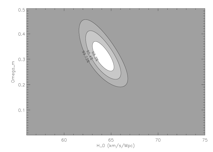
Figure 2: Confidence limits for the estimation of parameters for the $\Lambda$CDM model, with $\Omega_{\Lambda}=1-\Omega_{m}$.

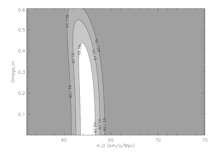
Figure 3: Confidence limits for the estimation of parameters for the Fractal Bubble Model .

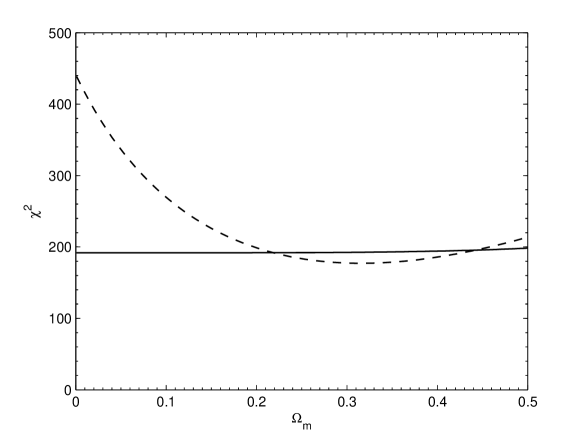
Figure 4: A slice of the confidence plot for the Fractal Bubble Model at its best–fit value $H_{\lower 2.0pt\hbox{$\scriptstyle 0$}}=62.683$ (solid line) for $0\leq\Omega_{m}\leq 0.5$, and for the $\Lambda$CDM model at its best–fit value $H_{\lower 2.0pt\hbox{$\scriptstyle 0$}}=64.145$ (dashed line).

A good fit for the $\Lambda$CDM model was at $H_{\lower 2.0pt\hbox{$\scriptstyle 0$}}=65\,\hbox{km}\;\,\hbox{sec}^{-1}\,\hbox{Mpc}^{-1}$ and $\Omega_{m}=0.27$ with ($\chi^{2}=178$) (Riess et al. 2004). For the Fractal Bubble Model the best fit values are at $H_{\lower 2.0pt\hbox{$\scriptstyle 0$}}=62.7^{+0.6\,(1\sigma),\;+1.1\,(2\sigma)}_{-1.1\,(1\sigma),\;-1.7\,(2\sigma)}\,\hbox{km}\;\,\hbox{sec}^{-1}\,\hbox{Mpc}^{-1}$ and include the $1\sigma$ range $\Omega_{m}<0.44$ ($\chi^{2}=191.7$). The value of $\chi^{2}$ is affected so little by the value of $\Omega_{m}$ in this range that we do not quote a single best–fit value. The $2\sigma$ confidence limit is $\Omega_{m}<0.55$. $\Omega_{m}$ can be made arbitrarily small within the $1\sigma$ bounds. Since recalibrated primordial nucleosynthesis bounds for baryonic matter are typically in the range $\Omega_{b}\mathop{\sim}\limits 0.02$–$0.13$, we see that the supernova data fit well for the FB model regardless of whether or not there is cold dark matter in addition to baryonic matter.

A Bayes factor for the two models can be calculated from the data by

$$B_{12}=\frac{\int{\rm d}H_{\lower 2.0pt\hbox{$\scriptstyle 0$}}\,\int{\rm d}\Omega_{m}\exp(-\chi_{\hbox{\sevenrm model 1}}^{2}/2)}{\int{\rm d}H_{\lower 2.0pt\hbox{$\scriptstyle 0$}}\,\int{\rm d}\Omega_{m}\exp(-\chi_{\hbox{\sevenrm model 2}}^{2}/2)}\,.$$ (9)

This result can be interpreted using Table LABEL:tab:bayesfac. For very wide priors, namely $0.001\leq\Omega_{m}\leq 0.5$ and $55\leq H_{\lower 2.0pt\hbox{$\scriptstyle 0$}}\leq 75\,\hbox{km}\;\,\hbox{sec}^{-1}\,\hbox{Mpc}^{-1}$, the Bayes factor is 396 in favour of $\Lambda$CDM. However, we note that the Bayes factor is very sensitive to the range chosen for the priors, since the best–fit values for the two models are include quite distinct values of $\Omega_{m}$. This is seen in Table LABEL:tab:bayescomp, where narrower priors are used for $H_{\lower 2.0pt\hbox{$\scriptstyle 0$}}$, and a variety of priors for $\Omega_{m}$. The examples with baryonic matter only use values of the baryon matter density from primordial nucleosynthesis bounds, as specifically recalibrated for the FB model by Wiltshire (2005b): it is found that the density fraction of ordinary baryonic matter is 2–3 times that which is conventionally obtained, and typically $\Omega_{b}\mathop{\sim}\limits 0.1$ is expected.

Table 1: Interpretation of Bayes Factors

$B_{12}$	Strength of evidence for $H_{1}$ over $H_{2}$
1 to 3	Not worth more than a bare mention
3 to 20	Positive
20 to 150	Strong
$>150$	Very Strong

Table 2: Bayes Factor comparison of a $\Omega_{\Lambda}=1-\Omega_{m}$ $\Lambda$CDM model versus the FB model with a fixed prior for $H_{\lower 2.0pt\hbox{$\scriptstyle 0$}}=100h\,\hbox{km}\;\,\hbox{sec}^{-1}\,\hbox{Mpc}^{-1}$, $58\leq h\leq 72$, and varying priors for $\Omega_{m}$. The baryonic density parameter bounds for the FB model are determined by Wiltshire (2005b).

$\Omega_{m}$ prior	Model type	$B_{\hbox{\sevenrm($\scriptstyle\Lambda$CDM):(FBM)}}$	Model favoured
$0.01\leq\Omega_{m}\leq 0.5$	Wide priors	396	$\Lambda$CDM
$0.2\leq\Omega_{m}\leq 0.3$	favoured CDM range	649	$\Lambda$CDM
$0.3\leq\Omega_{m}\leq 0.5$	high density CDM	1014	$\Lambda$CDM
$0.01\leq\Omega_{m}\leq 0.2$	low density CDM	0.53	FBM (slightly)
$0.08\leq\Omega_{m}\leq 0.13$	baryonic matter, low D/H	$2.6\times 10^{-5}$	FBM
$0.02\leq\Omega_{m}\leq 0.06$	baryonic matter, high D/H	$1.3\times 10^{-14}$	FBM

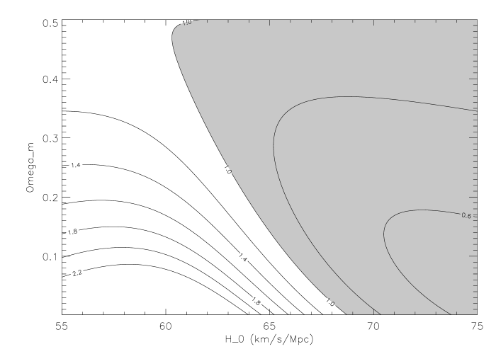
Figure 5: A contour plot of $\chi^{2}_{\hbox{\sevenrm FBM}}/\chi^{2}_{\hbox{\sevenrm$\scriptstyle\Lambda$CDM}}$ for Fractal Bubble Model vs the $\Lambda$CDM model. The Fractal Bubble Model fares better in the lower left region (white), while the $\Lambda$CDM model is favoured in the upper right region (lightly shaded).

To characterise the parameter space better, we also give a plot of the $\chi^{2}$ value as a function of $\Omega_{m}$ for the best–fit value of $H_{\lower 2.0pt\hbox{$\scriptstyle 0$}}$ in each model in Fig. 4, and similarly plot $\chi^{2}_{\hbox{\sevenrm FBM}}/\chi^{2}_{\hbox{\sevenrm$\scriptstyle\Lambda$CDM}}$ for the two models for the whole parameter space spanned by $\Omega_{m}$ and $H_{\lower 2.0pt\hbox{$\scriptstyle 0$}}$ in Fig. 5. The Fractal Bubble Model is favoured for lower values of $\Omega_{m}$ and $H_{\lower 2.0pt\hbox{$\scriptstyle 0$}}$, and $\Lambda$CDM for higher values of both parameters. Also observe from Fig. 4 how insensitive the FB model is to the value of $\Omega_{m}$ in the range $0<\Omega_{m}\lesssim 0.5$.

4 Data reduction

While SNeIa serve as excellent standard candles there is some dispersion observed in their absolute magnitudes. However, a relation first proposed by Phillips (1993), relates the absolute magnitude, $M$, to the change in apparent magnitude from peak to 15 days after peak, $\Delta m_{15}$, as measured by clocks in the rest frame of the supernova. Various methods have been used to fit light curves to obtain absolute magnitudes (Drell, Loredo & Wasserman 2000, Tonry 2003).

It is also well demonstrated that redshift causes a broadening of light curves (Leibundgut 1996) corresponding to the phenomenon of cosmic time dilation. In standard cosmology the redshift is entirely attributable to cosmic expansion. It is then a simple matter to transform the observed light curve to the rest frame. In the FB model

$$1+z=\frac{\widetilde{a}_{\lower 2.0pt\hbox{$\scriptstyle 0$}}\gamma(\tau_{\hbox{\sevenrm emit}})}{\widetilde{a}(\tau_{\hbox{\sevenrm emit}})\gamma_{\lower 2.0pt\hbox{$\scriptstyle 0$}}}\,,$$ (10)

so that the measured redshift differs from that inferred from (1). However, for null geodesics the transformation to the rest frame only involves only the overall $(1+z)$ factor of the measured redshift, so that the light curve broadening determination will be unaffected. Only measurements which involved some independent determination of $\gamma(\tau_{\hbox{\sevenrm emit}})/\gamma_{\lower 2.0pt\hbox{$\scriptstyle 0$}}$, would lead to measurable differences between this model and models based on the conventional identification of clock rates.

It is impossible to comment on the Phillips relations, and other related aspects of data–fitting, without access to the raw data. However, since these are relations are empirical, it is not likely that there would be significant differences in the FB model.

The only likely systematic errors that are as yet unaccounted for in reducing the data for comparison with the FB model are those effects directly related to the inhomogeneous geometry. The metric (1) represents an average geometry only, and for the redshifts which presently constitute the bulk of the sample, a better understanding of intermediate scales in the fitting problem may be required. Studies of local voids – at scales well within the bubble SS– do reveal that measurable effects on cosmological parameters are possible (Tomita 2001). In the present model, the average rate of expansion of typical $30h^{-1}$ Mpc voids would differ from that of much larger voids. While the dominant effect on luminosity distances suggested here is a new effect due to the identification of an alternative homogeneous time parameter in solving the “fitting problem”, further scale dependent corrections in the fractal geometry are certainly to be expected.

5 Conclusion

From the standard Bayesian analysis with wide priors we would conclude that on the basis of the “Gold data set” of (Riess et al. 2004), the standard $\Lambda$CDM model is very strongly favoured over the FB model. Nonetheless, this conclusion depends strongly on the priors assumed, as illustrated by Table LABEL:tab:bayescomp and Figs. 4 and 5. We must also bear in mind that the average geometry (1)–(3) is just a first approximation to the fitting problem. A better understanding of the differential expansion rates of different characteristic sizes of voids in the inhomogeneous geometry may improve the fit of the FB model at those redshifts which are most significant for the claims of cosmic acceleration, rather than a nearly empty universe deceleration. The FB model has other significant advantages in terms of it greatly increased expansion age (Wiltshire 2005a), which has the potential to explain the formation of structure at large redshifts. Thus it should be considered as a serious alternative to models with dark energy, quite apart from its intrinsic appeal of being a model based simply on general relativity and primordial inflation without needing exotic dark energy, the presence of which at the present epoch would be a mystery to physics.

In the end, nature is the final arbiter, and future supernova observations at higher redshifts, such as those of the SNAP mission, will certainly be able to much more decisively distinguish between the FB model and $\Lambda$CDM, given the significantly more rapid deceleration of $\Lambda$CDM at redshifts $z>2$.

Acknowledgements: This work was supported by the Marsden Fund of the Royal Society of New Zealand. We thank Michael Albrow for helpful comments.

Note added: After this work appeared an independent SneIa data analysis of the Milne universe – considered as an approximation to a variety of alternative theories – has been performed (Sethi, Dev & Jain 2005). They obtain a comfortable fit just as we would expect from our results given that the FB model mimics a Milne universe for $z<2$.

References

- Drell, Loredo & Wasserman (1999) Drell, P.S., Loredo, T.J. and Wasserman, I. 2000, “Type Ia supernovae, evolution, and the cosmological constant”, ApJ 530, 593.
- Ellis & Stoeger (1987) Ellis, G.F.R. and Stoeger, W. 1987, “The fitting problem in cosmology”, Class. Quantum Grav. 4, 1697.
- Kolb (2005) Kolb, E.W., Matarrese, S., Notari, A. and Riotto, A. 2005, “Primordial inflation explains why the universe is accelerating today”, arXiv:hep-th/0503117.
- Leibundgut (1996) Leibundgut, B. 1996, “Time dilation in the light curve of the distant type Ia supernovae SN 1995K”, ApJ466, L21.
- Ng & Wiltshire (2001) Ng, S.C.C. and Wiltshire, D.L. 2001, “Future supernova probes of quintessence”, Phys. Rev. D 64, 123519.
- Phillips (1993) Phillips, M.M. 1993, “The absolute magnitudes of Type IA supernovae”, ApJ 413, L105.
- (7) Riess, A.G., et al. 2004, “Type Ia supernova discoveries at z1 from the Hubble Space Telescope: Evidence for past deceleration and constraints on dark energy evolution”, ApJ 607, 665.
- (8) Sethi, G., Dev, A., and Jain, D. 2005, “Cosmological constraints on a power law universe”, arXiv:astro-ph/0506255.
- (9) Tomita, K. 2001, “A local void and the accelerating universe”, MNRAS 326, 287.
- Tonry et al. (2003) Tonry, J.L. et al. 2003, “Cosmological results from high-z supernovae”, ApJ 594 , 1.
- Wiltshire (2005) Wiltshire, D.L. 2005a, “Viable inhomogeneous model universe without dark energy from primordial inflation”, arXiv:gr-qc/0503099.
- Wiltshire (2005) Wiltshire, D.L. 2005b, “Fractal bubble universe: Principles and dynamics of cosmology without dark energy”, in preparation.