The Kinetic Sunyaev-Zel’dovich Effect from Reionization

Abstract

During the epoch of reionization, local variations in the ionized fraction (patchiness) imprint arcminute-scale temperature anisotropies in the CMB through the kinetic Sunyaev-Zel’dovich (kSZ) effect. We employ an improved version of an analytic model of reionization devised in Furlanetto et al. (2004b) to calculate the kSZ anisotropy from patchy reionization. This model uses extended Press-Schechter theory to determine the distribution and evolution of H II bubbles and produces qualitatively similar reionization histories to those seen in recent numerical simulations. We find that the angular power spectrum of the kSZ anisotropies depends strongly on the size distribution of the H II bubbles and on the duration of reionization. In addition, we show that upcoming measurements of the kSZ effect should be able to distinguish between several popular reionization scenarios. In particular, the amplitude of the patchy power spectrum for reionization scenarios in which the IGM is significantly ionized by Population III stars (or by mini-quasars/decaying particles) can be larger (or smaller) by over a factor of 3 than the amplitude in more traditional reionization histories (with temperature anisotropies that range between $0.5$ and $3~{}\mu K$ at ${\it l}=5000$). We highlight the differences in the kSZ signal between many possible reionization morphologies and discuss the constraints that future observations of the kSZ will place on this epoch.

1. Introduction

Scattering of cosmic microwave background (CMB) photons off objects after recombination imprints hot and cold spots in the CMB. Measurement of these secondary anisotropies will elucidate details of the formation and evolution of structure in the universe, including the morphology of reionization. CMB detectors (such as BIMA, CBI and soon ACT and SPT) are beginning to reach small enough scales ($\lesssim 5$ arcminutes) where the primordial temperature anisotropies no longer dominate the secondaries. On these scales, the principal secondary anisotropy at most wavelengths is the thermal Sunyaev-Zel’dovich (tSZ) effect, which comes from scattering off hot intracluster gas (Zel’dovich & Sunyaev, 1969). The tSZ signal is dominated by nearby clusters and therefore is not optimal for studying the high-redshift universe. However, the unique frequency dependence of the tSZ anisotropies (vanishing at $\sim 217$ GHz) facilitates their removal from the signal. This may allow future CMB missions to detect the kinetic Sunyaev-Zel’dovich (kSZ) effect—owing to scattering off of objects with bulk peculiar motions (Sunyaev & Zel’dovich, 1980).

During the epoch of reionization, local variations in the ionized fraction (or patchiness) contribute to the kSZ signal. The anisotropies produced by this patchiness have been calculated for various analytic models of reionization (Gruzinov & Hu, 1998; Knox et al., 1998; Valageas et al., 2001; Santos et al., 2003). These treatments differ considerably in their description of this epoch, but most find that the kSZ temperature anisotropies produced during reionization have a similar amplitude to the kSZ anisotropies produced after reionization. This suggests that observations of the kSZ effect might provide important constraints on the reionization epoch.

Existing probes of this era have provided few definitive answers about reionization. Observations of Ly$\alpha$ absorption in the spectra of high-redshift quasars indicate that it ends at $z\sim 6$ (Becker et al., 2001; Fan et al., 2002; White et al., 2003; Sokasian et al., 2003; Wyithe & Loeb, 2004; Mesinger & Haiman, 2004; Oh & Furlanetto, 2005). The main difficulty with these measurements is that the Ly$\alpha$ optical depth is extremely large in a neutral medium (Gunn & Peterson, 1965), making it difficult to place strong constraints when the neutral fraction exceeds $\sim 10^{-3}$. On the other hand, measurements of the cosmic microwave background by the Wilkinson Microwave Anisotropy Probe (WMAP) suggest a high optical depth to electron scattering, apparently requiring reionization to begin at $z\gtrsim 14$ (Kogut et al., 2003; Spergel et al., 2003). Unfortunately, the WMAP data provide only an integral constraint on the reionization history.

In this paper, we employ the analytic model outlined in Furlanetto et al. (2004b, hereafter FZH04) to calculate the kSZ signal for many different reionization histories. Most analytic models of reionization are based on the growth of H II regions around individual galaxies or quasars (Arons & Wingert, 1972; Barkana & Loeb, 2001). This contrasts with current state-of-the-art simulations (Sokasian et al., 2003, 2004; Ciardi et al., 2003; Furlanetto et al., 2004d), which find a relatively small number of large ionized regions around clusters of sources. Moreover, in these simulations, reionization proceeds from high to low density regions, implying that recombinations play only a secondary role in determining the morphology of reionization; instead, large-scale bias dominates. The model we employ produces similar reionization histories to those seen in these simulations.

This paper is organized as follows. We outline the formalism for calculating the kSZ power spectrum in §2. In §3, we review and improve upon the reionization model first developed in FZH04. This model is able to produce a range of possible morphologies for reionization. We then calculate the kSZ power spectrum for several different reionization scenarios, highlighting the observable differences between them (§4), and discuss whether future observations of the kSZ effect will be able to constrain the history of reionization (§5).

In our calculations, we assume a cosmology with $\Omega_{m}=0.3$, $\Omega_{\Lambda}=0.7$, $\Omega_{b}=0.046$, $H=100h\mbox{ km s${}^{-1}$ Mpc${}^{-1}$}$ (with $h=0.7$), $n=1$, and $\sigma_{8}=0.9$, consistent with the most recent measurements (Spergel et al., 2003).

2. The kinetic SZ effect

Thomson scattering of CMB photons off free electrons with a bulk peculiar velocity produces a temperature anisotropy along the line of sight ${\bf\hat{n}}$:

$$\frac{\Delta T}{T}({\bf\hat{n}})=\sigma_{T}\;\int{{\rm d}\eta\;e^{-\tau(\eta)}\;a\,n_{e}\;{\bf\hat{n}}\cdot{\bf v}},$$ (1)

where $a$ is the scale factor, $\tau(\eta)$ is the Thomson optical depth to the scatterer at conformal time $\eta$, ${\bf v}({\bf\hat{n}},\eta)$ is the peculiar velocity of the scatterer, and the electron number density is

$$n_{e}(\eta,{\bf\hat{n}})=\bar{n}_{e}(\eta)\;\bar{x}_{i}(\eta)\;[1+\delta_{b}(\eta,{\bf\hat{n}})+\delta_{x}(\eta,{\bf\hat{n}})].$$ (2)

Here, $\bar{n}_{e}$ is the average number density of electrons (both within atomic systems and free), $\bar{x}_{i}$ is the global ionized fraction, and $\delta_{b}$ and $\delta_{x}$ are the overdensities in the baryonic mass and the ionized fraction (we reserve $\delta$ for the matter overdensity). The two-point correlation function $w(\theta)=\langle\frac{\Delta T}{T}({\bf\hat{n}})\frac{\Delta T}{T}({\bf\hat{n}^{\prime}})\rangle$ is

$$w(\theta) = [\sigma_{T}\,\bar{n}_{e}(\eta_{0})]^{2}\;\int d\eta\;{W(\eta)}\int d\eta^{\prime}\,{W(\eta^{\prime})}\,\hat{n}_{i}\,\hat{n}_{j}^{\prime}$$ (3)

$$\times\langle q^{i}\,{q^{\prime}}^{j}\rangle(\sqrt{\theta^{2}\,(\eta_{0}-\eta)^{2}+(\eta-\eta^{\prime})^{2}}\,,\,\eta),$$

where ${\bf q}({{\bf x}},\eta)={\bf v}\,(1+\delta_{b}+\delta_{x})$, $W(\eta)=a^{-2}\,\bar{x}_{i}^{2}\,e^{-\tau}$, and repeated indexes are summed. In equation (3), correlations between points separated by the vector $(\Delta\eta,\Delta x)$ are treated as equivalent to points separated by $(0,\Delta x)$. While this approximation should be adequate for our purposes, we substitute $\sqrt{\langle{\bf q}\,{\bf q}^{\prime}\rangle({\bf x},\eta)~{}\langle{\bf q}\,{\bf q}^{\prime}\rangle({\bf x},\eta^{\prime})}$ for $\langle{\bf q}\,{\bf q}^{\prime}\rangle(x,\eta)$ to capture better the $\eta$ dependence.

Simplifications to equation (3) are most apparent in Fourier space: equation (1) involves the integral $\int{d\eta\,W(\eta)\,{\bf\hat{n}}\cdot{\bf q}({\bf k})\,e^{{\it i}{\bf k}\cdot\hat{n}\,(\eta_{0}-\eta)}}$, which suffers severe cancellation for ${\bf k}$ along the line of sight. Thus, for modes much shorter than the thickness of the window function and in the flat sky approximation ($k={\it l}/x$, $x=\eta_{0}-\eta$), the Fourier space version of equation (3) reduces to (Kaiser, 1992; Jaffe & Kamionkowski, 1998)

$$C_{\it l}=(\sigma_{T}\,\bar{n}_{e}(\eta_{0}))^{2}\;\int{\frac{d\eta}{x^{2}}\;{W(\eta)}^{2}\,P_{q_{\perp}}({\it l}/x,\eta)},$$ (4)

where $\langle{\bf q}_{\perp}({\bf k})\cdot{\bf q}^{*}_{\perp}({\bf k}^{\prime})\rangle=2\,(2\pi)^{3}\,\delta^{3}_{D}({\bf k}-{\bf k}^{\prime})\,P_{q_{\perp}}({\bf k})$ and ${\bf q}_{\perp}({\bf k})$ is the projection of ${\bf q}({{\bf k}})$ perpendicular to ${{\bf k}}$,

$${\bf q}_{\perp}({{\bf k}}) = \int\frac{d^{3}{{\bf k}^{\prime}}}{(2\pi)^{3}}\left[{\bf\hat{k}}^{\prime}-{\mu^{\prime}}~{}{\bf\hat{k}}\right]\,v({\bf k}^{\prime})$$ (5)

$$\times\left[\delta_{b}(|{\bf k}-{\bf k}^{\prime}|)+\delta_{x}(|{\bf k}-{\bf k}^{\prime}|)\right].$$

Here, $\mu^{\prime}={\bf\hat{k}}\cdot{\bf\hat{k}}^{\prime}$ and ${\bf v}({{\bf k}})=v(k)\,{\bf\hat{k}}$ where ${\bf v}({\bf k})$ is the linear theory velocity field [${\bf v}({\bf k})={\it i}\,{\bf\hat{k}}\,(f\dot{a}/k)\,\delta^{\rm lin}(k,\eta)$, with $f=d\log D/d\log a$ and $D$ the growth factor]. The linear theory velocity suffices because nonlinear contributions to the the velocity of objects are negligible in the early universe. Cooray & Chen (2002) estimated the nonlinear velocity contribution to the kSZ power spectrum by utilizing virial velocity arguments for spherically-symmetric halos. They found that this contributes about an order of magnitude less signal than the kSZ effect from the linear theory velocities. At the high redshifts relevant to reionization, the impact of nonlinear velocities will be even less important.

To simplify equation (4), note that the three-point terms in $P_{q_{\perp}}$ are negligible because they involve correlations with just ${\bf v}({\bf k})$ at one point, and ${\bf v}_{\perp}({\bf k})={\bf 0}$ by definition. This leaves three four-point correlation functions. We can decompose these into a sum of all possible pairs of two-point functions along with the connected fourth moments (Ma & Fry, 2002; Santos et al., 2003)

$$P_{q_{\perp}}(k) = \frac{1}{2}\sum_{a,b=\delta_{b},\delta_{x}}\int\frac{{\rm d}^{3}{\bf k^{\prime}}}{(2\pi)^{3}}[(1-{\mu^{\prime}}^{2})P_{vv}(k^{\prime})P_{ab}(|{\bf k}-{\bf k}^{\prime}|)$$ (6)

$$-\frac{(1-{\mu^{\prime}}^{2})\,k^{\prime}}{|{\bf k}-{\bf k}^{\prime}|}P_{av}(k^{\prime})P_{bv}(|{\bf k}-{\bf k}^{\prime}|)]$$

$$+\int\frac{{\rm d}{\bf k}^{\prime}~{}{\rm d}{\bf k}^{\prime\prime}}{(2\pi)^{6}}\,\sqrt{(1-{\mu^{\prime}}^{2})\,(1-{\mu^{\prime\prime}}^{2})}\,{\rm cos}(\phi^{\prime}-\phi^{\prime\prime})$$

$$\times P_{\delta_{a}\delta_{b}vv}({\bf k}-{\bf k}^{\prime},-{\bf k}-{\bf k}^{\prime\prime},{\bf k}^{\prime},{\bf k}^{\prime\prime}),$$

where $P_{\delta_{*}\delta_{*}vv}$ is the connected fourth moment and $\{\phi^{\prime},\phi^{\prime\prime}\}$ are the polar angles of the vectors $\{{\bf k}^{\prime},{\bf k}^{\prime\prime}\}$. In the halo model and in our reionization model, where H II bubbles are assumed spherical and correlations between objects are handled similarly to those in the halo model, $P_{\delta_{*}\delta_{*}vv}$ does not depend on $\phi^{\prime}$. Therefore the contribution from the connected fourth moments vanish. Ma & Fry (2002) verify in simulations that the contribution to $P_{q_{\perp}}$ from $P_{\delta_{b}\delta_{b}vv}$ is indeed negligible. Zahn et al. (2005) compute the kSZ for a nearly identical distribution of bubbles sizes as we do, but allow for more complicated configurations of bubbles. The agreement of our kSZ signal with theirs (see Fig. 5 and §4.1 below), suggests that the connected fourth moments involving $\delta_{x}$ are also small and that this is not just a byproduct of our simplified model for reionization.

To further simplify equation (6), we drop the cross correlation terms $P_{\delta_{b}v}$ and $P_{\delta_{x}v}$. Even if $P_{\delta_{*}\delta_{*}}\,P_{vv}$ is comparable to $P_{\delta_{*}v}\,P_{\delta_{*}v}$, equation (6) is dominated by $k^{\prime}$ near zero at the scales of interest, $k\gtrsim 1\,{\rm Mpc}^{-1}$ (noting that $P_{\delta_{\rm lin}\delta_{\rm lin}}$ and $P_{\delta_{*}\delta_{\rm lin}}$ scale roughly as $k^{\prime-3}$ for $k^{\prime}\gtrsim 0.05\,{\rm Mpc}^{-1}$ and that $v\propto\delta_{\rm lin}/k^{\prime}$ ). The terms involving $P_{\delta_{*}v}$ are ${\cal O}(k^{\prime}/k)$ and are therefore suppressed.

This argument suggests a further simplification for the large $k$ modes of interest. Isolating the case $a=b=\delta_{b}$ in the sum in equation (6), dropping terms of ${\cal O}(k^{\prime}/k)$, and evaluating the angular integral, we find

$$P_{q_{\perp},a=b=\delta_{b}}(k)=\frac{1}{3}\,v_{rms}^{2}\,P_{\delta_{b}\delta_{b}}(k),$$ (7)

where $v_{rms}^{2}=\int{\frac{k^{2}dk}{2\pi^{2}}P_{vv}(k)}$ (Hu, 2000; Ma & Fry, 2002). This $P_{\delta_{b}\delta_{b}}$ contribution to $P_{q_{\perp}}$ is the dominant term for uniform reionization and is sometimes called the Ostriker-Vishniac effect (OV). Traditionally, this effect is calculated using linear theory (Ostriker & Vishniac, 1986; Dodelson & Jubas, 1993). Hu (2000) first calculated the nonlinear OV effect, demonstrating that at ${\it l}\sim 10^{4}$ the signal is significantly increased by nonlinearities. We use the halo model (Cooray & Sheth, 2002) to construct $P_{\delta\delta}$ – which we then employ to calculate the term $P_{\delta_{b}\delta_{b}}$ in equation (7). Unfortunately, calculating $P_{\delta_{b}\delta_{b}}$ also requires knowledge of the distribution of baryons inside halos: at large overdensities, baryonic matter does not trace the dark matter. To model the baryon distribution, we employ a filter function $F(x)$ such that $P_{\delta_{b}\delta_{b}}(k)=F(k)P_{\delta\delta}(k)$, where $P_{\delta\delta}$ is the nonlinear matter power spectrum. The function $F(k)$ filters large $k$ contributions from the dark matter power spectrum, such that the baryonic matter is not as clumpy as the dark matter (see Appendix A for details).

Hu (2000) uses the same method to calculate the OV. Our OV signal agrees well with the analytic calculation of Zhang et al. (2004), which uses a similar method but also includes the nonlinear velocity field. Ma & Fry (2002) and Cooray & Sheth (2002) employ a different method to calculate the OV effect, modeling the gas distribution in halos with a $\beta$ profile $\rho(r)=A\,[1+(r/r_{c})^{2}]^{-3\beta/2}$ or a similar function. Their calculation results in a slightly smaller signal. Perhaps a superior method for calculating the OV is through hydrodynamic simulations. Such simulations must cover a huge dynamic range, resolving nearby halos and large scale structure at high redshifts. Simulations tend to agree relatively well with the predictions of these analytic methods at high-$l$ (da Silva et al., 2001; White et al., 2002; Zahn et al., 2005), but they predict less signal at $l<5000$. Such deviations are less important for studying secondary anisotropies because the primordial anisotropies dominate at these scales. (Contamination of the primordial anisotropies and the resulting bias in cosmological parameter estimation is a different matter.)

The other two terms contributing to $P_{q_{\perp}}$ involve integrals over $P_{vv}\,P_{\delta_{x}\delta_{x}}$ – the term normally included in calculations of patchy reionization – and the cross correlation $2P_{vv}\,P_{\delta_{b}\delta_{x}}$ – ignored in existing calculations, but possibly significant if the H II bubbles occur in overdense regions as simulations suggest. We refer to these two terms as the “patchy” terms. Since the universe reionizes quickly in some of our models (see Figure 3), the assumption implicit in equation (4) – $k^{-1}$ is much shorter than the distance over which the window function changes appreciably – may break down at some relevant l. This is not a concern for the OV effect, where only a small portion of the signal comes from the reionization epoch. Simple estimates suggest that at scales where the kSZ effect dominates over the primordial anisotropies (${\it l}\gtrsim 5000$), equation (4) should be an adequate approximation. However, to be safe, we do the calculation in configuration space (eq. 3). Additional details concerning the configuration space calculation are given in Appendix B.

Hu (2000) showed that the high-l polarization resulting from scattering of the primordial and kinetic quadrupoles off perturbations in the density and ionized fraction have negligible amplitude ($10^{-3}-10^{-2}\mu K$). This results from the small magnitude of the quadrupole anisotropies. The high-l polarization signal from reionization is thus too small to affect upcoming measurements of B-parity polarization from gravitational lensing or from gravitational waves. Therefore, we only discuss the temperature anisotropies here.

3. H II regions during reionization

Recent numerical simulations (e.g., Sokasian et al. 2003, 2004; Ciardi et al. 2003) show that reionization proceeds “inside-out” from high density clusters of sources to voids, at least when the sources resemble star-forming galaxies (e.g., Springel & Hernquist 2003; Hernquist & Springel 2003). We therefore associate H II regions with large-scale overdensities. We assume that a galaxy of mass $m_{\rm gal}$ can ionize a mass $\zeta m_{\rm gal}$, where $\zeta$ is a constant that depends on: the efficiency of ionizing photon production, the escape fraction, the star formation efficiency, and the number of recombinations. Values of $\zeta\lesssim 40$ are reasonable for normal star formation, but very massive stars can increase the efficiency by an order of magnitude (Bromm et al., 2001b). The criterion for a region to be ionized by the galaxies contained inside it is then $f_{\rm coll}>\zeta^{-1}$, where $f_{\rm coll}$ is the fraction of mass bound to halos above some $m_{\rm min}$. We will normally assume that this minimum mass corresponds to a virial temperature of $10^{4}\mbox{ K}$, at which point hydrogen line cooling becomes efficient. In the extended Press-Schechter model (Bond et al., 1991; Lacey & Cole, 1993) the collapse fraction of halos above the critical mass $m_{\rm min}$ in a region of mean overdensity $\delta_{m}$ is

$$f_{\rm coll}={\rm erfc}\left(\frac{\delta_{c}-\delta_{m}}{\sqrt{2\left[\,\sigma^{2}_{\rm min}-\sigma^{2}(m,z)\right]}}\right),$$ (8)

where $\sigma^{2}(m,z)$ is the variance of density fluctuations on the scale $m$, $\sigma^{2}_{\rm min}\equiv\sigma^{2}(m_{\rm min},z)$ and $\delta_{c}\approx 1.686$, the critical density for collapse. With this equation for the collapse fraction, we can write a condition on the mean overdensity within an ionized region of mass $m$,

$$\delta_{m}\geq\delta_{B}(m,z)\equiv\delta_{c}-\sqrt{2}K(\zeta)[\sigma^{2}_{\rm min}-\sigma^{2}(m,z)]^{1/2},$$ (9)

where $K(\zeta)={\rm erf}^{-1}\left(1-\zeta^{-1}\right)$.

FZH04 showed how to construct the mass function of H II regions from $\delta_{B}$ in an analogous way to the halo mass function (Press & Schechter, 1974; Bond et al., 1991). The barrier in equation (9) is well approximated by a linear function in $\sigma^{2}$, $\delta_{B}\approx B(m)=B_{0}+B_{1}\sigma^{2}(m)$, where the redshift dependence is implicit. In that case, the mass function has an analytic expression (Sheth, 1998):

$$n(m)=\sqrt{\frac{2}{\pi}}\ \frac{\bar{\rho}}{m^{2}}\ \left|\frac{{\rm d}\ln\sigma}{{\rm d}\ln m}\right|\ \frac{B_{0}}{\sigma(m)}\exp\left[-\frac{B^{2}(m)}{2\sigma^{2}(m)}\right],$$ (10)

where $\bar{\rho}$ is the mean density of the universe. Equation (10) gives the comoving number density of H II regions with masses in the range $(m,m+dm)$. This result is rederived in Appendix C. The crucial difference between this formula and the standard Press-Schechter mass function occurs because $\delta_{B}$ is a (decreasing) function of $m$. The barrier is more difficult to cross as one goes to smaller scales, which gives the bubbles a characteristic size that depends primarily on $\bar{x}_{i}$. The one point function $\bar{x}_{i}(z)$ for the linear barrier is (Appendix C)

$$Q(z)\equiv\bar{x}_{i}(z) = \frac{1}{2}\,e^{-2\,B_{0}\,B_{1}}\,{\rm erfc}\left(\frac{B_{0}-B_{1}\sigma_{\rm min}^{2}}{\sqrt{2\,\sigma_{\rm min}^{2}}}\right)$$ (11)

$$+\,\frac{1}{2}\,{\rm erfc}\left(\frac{B_{0}+B_{1}\sigma_{\rm min}^{2}}{\sqrt{2\,\sigma_{\rm min}^{2}}}\right).$$

This equation agrees extremely well with the $Q(z)$ one finds with the full barrier (equation 9).

All the quantities we want to calculate are well-defined in this model. In addition, since the typical bubble size is usually larger than the scale of nonlinearities, calculating the desired patchy correlation functions is simply a matter of exploring the properties of a Gaussian random field.

3.1. Bias of the H II Regions

Unfortunately, there was an inaccuracy in the formula FZH04 used for the linear bias (their eq. 22) that caused them to underestimate the bias. (Note that the expression in Sheth & Tormen 2002 is also incorrect.) To compute the correct bias, we consider how the bubble number density $n(m)$ varies with the underlying (large-scale) density. This is straightforward for a linear barrier, because the barrier remains linear after a translation by the origin.

Suppose we are in a region of linear-extrapolated matter overdensity $\delta_{R}$ and variance $\sigma_{R}$ at a smoothing scale $R$; note that the linear-extrapolated matter overdensity at redshift $z$ is $\delta_{R}\,D(z)$ (we adopt this notation for $\delta$ only for this section). The comoving number density of bubbles $n(m|\delta_{R},\sigma_{R})$ is simply the usual expression, equation (10), with the replacements

$$\sigma(m)^{2} \rightarrow \sigma(m)^{2}-{\sigma_{R}}^{2},$$

$$B(m,z) \rightarrow B(m,z)-\delta_{R},$$

$$B_{0} \rightarrow B_{0}+B_{1}\,{\sigma_{R}}^{2}-\delta_{R}.$$

Linearizing the resulting expression and noting that the Eulerian overdense region is larger by a factor of $(1+\delta_{R})$ (Mo & White, 1996) , we find

$$\delta_{x}(m) = \delta_{R}\,D(z)\,\left[1+\frac{B(m)/\sigma(m)^{2}-1/B_{0}}{D(z)}\right]$$ (12)

$$+\frac{B_{1}\,\sigma_{R}^{2}}{B_{0}},$$

where $\delta_{x}(m)$ is the overdensity of bubbles with mass $m$ [note that $\delta_{x}=\int dm\,n(m)\,\delta_{x}(m)$]. The last term is only significant if $R$ is small or if we are so close to reionization that $B_{1}\sigma_{R}^{2}\sim B_{0}$. If we neglect this term, the linear bias is thus

$$b_{x}(m)=1+\frac{B(m)/\sigma^{2}(m)-1/B_{0}}{D(z)}.$$ (13)

Interestingly, for sufficiently small bubbles $b_{x}<0$. This means that small bubbles become rare in large overdensities and more common in underdense regions. Physically, this occurs because overdense regions are more advanced in the reionization process such that the small bubbles have already merged with larger H II regions. During the late stages of reionization, only the deepest voids contain galaxies isolated enough to create small bubbles.

Finally, we define the average bias

$$\bar{b}_{x}\equiv Q^{-1}\int dm\,n(m)\,V(m)\,b_{x}(m),$$ (14)

which is the bias averaged over the bubble filling factor. The average bias tends to be quite large throughout reionization, typically between $3<\bar{b}_{x}<10$. The (incorrect) prescription of FZH04 resulted in moderate bias $b_{x}\sim 1$ and thus underestimated the clustering of bubbles.

Working only to linear order in the expansion of $\delta_{R}$ can be problematic because the bias is so large. This is particularly true for $Q$ near unity. In this limit, even small overdensities can lead to the nonsensical result $x_{\delta}\approx Q\,[1+\bar{b}_{x}\,\delta_{R}\,D(z)]>1$, where $x_{\delta}$ is the ionized fraction in a region of overdensity $\delta_{R}$. For large $Q$, only the most underdense parts of the universe are not ionized, so $x_{\delta}$ cannot be well-approximated as a linear function in $\delta_{R}$; the linear bias tends to overpredict the clustering of bubbles. Conceptually, the problem is the same as those described in §3.1 of FZH04. The linear bias works much better for small $Q$. Fortunately, for large $Q$ the bubbles become so large that they are essentially uncorrelated and the bias is unimportant.

3.2. Autocorrelation of the Ionized Fraction

In the original derivation of $\langle x_{i}\,x_{i}^{\prime}\rangle$ and $\langle x_{i}\,\delta^{\prime}_{b}\rangle$, FZH04 used a Poisson model that allowed the bubbles to overlap. However, our expression for $n(m)$ (eq. 10) does not actually allow this to happen: the bubbles are explicitly constructed to be the largest contiguous ionized regions in the universe. Here, we construct improved versions of $\langle x_{i}\,x_{i}^{\prime}\rangle$ where overlap is forbidden.

Unfortunately, this poses a new set of problems. To compute the relevant integrals analytically, we must assume that the bubbles are spherical. This assumption tends to suppress the ionized fraction at distances around the average bubble radius. The reason is simple. Imagine that all the bubbles are the same size. Then reionization would be similar to packing oranges in a crate: there is no way to do so without leaving some gaps, because the oranges cannot overlap. In reality, the bubbles will not be perfectly spherical; some will be elongated and able to fill these gaps. The most reliable treatment is far from obvious. If we completely disallow overlap, the suppression of power at the characteristic radius of the bubbles causes significant (and spurious) ringing in the power spectrum. The other option is to allow for some amount of bubble overlap. Qualitatively, one could think of this as allowing the bubbles to deform and fill the gaps. However, this will overestimate the signal at scales near the bubble radii. Of course this problem becomes worse as $Q\rightarrow 1$ and overlap becomes more common.

Our solution is to allow bubble overlap only when the ionized fraction is small. Outside of this regime, we note that the characteristic bubble radius is $\gtrsim 5$ Mpc when overlap is significant at $Q(z)\gtrsim 0.5$. Figure 1 shows this explicitly: we plot the characteristic bubble radius (defined as the peak of $Vdn/d{\rm log}R$) as a function of the ionized fraction at several fixed redshifts. When the bubbles become large, the dark matter correlation function $\xi_{\delta\delta}(r)$ is so small on the relevant scales that we can ignore the correlations between bubbles regardless of the bias. Therefore, we break our solution into two regimes: in the first, the bubbles are small and both the one and two bubble terms, $P_{1}$ and $P_{2}$, are important. In the other, the bubbles are large and only the one bubble term $P_{1}$ is significant. We have

$$\langle x_{i}x_{i}\rangle(r) =\left\{\begin{array}[]{l r}(1-Q)\,P_{1}(r)+Q^{2}\;\;\;\;\;\;\;Q>\eta,\\ P_{1}(r)+P_{2}(r)\;\;\;\;\;\;\;{\rm otherwise},\end{array}\right.$$ (17)

where

$$P_{1}(r) = \int dm\,n(m)\,V_{0}(m,r),$$ (18)

$$P_{2}(r) = \int dm_{1}\,n(m_{1})\int d^{3}{\bf r_{1}}\int dm_{2}\,n(m_{2})$$ (19)

$$\times\,\int d^{3}{\bf r_{2}}\,[1+\xi({\bf r_{1}}-{\bf r_{2}}|m_{1},m_{2})].$$

Here, $V_{0}(m,r)$ is the volume within a sphere of mass $m$ that can encompass two points separated by a distance $r$. The ansatz $[1-Q]\,P_{1}(r)+Q^{2}$ for the large-bubble regime is meant to approximate the case when we can ignore correlations between bubbles; note that it obeys the necessary limits described in FZH04. However, our prescription does miss the less important large scale limit, $\langle x_{i}x_{i}^{\prime}\rangle-Q^{2}\rightarrow\bar{b}_{x}^{2}\,\langle\delta\delta^{\prime}\rangle$. This does not affect our calculation because $\langle\delta\delta^{\prime}\rangle$ and $\langle vv^{\prime}\rangle$ are so small on these scales – scales where the primordial anisotropies dominate anyway.

The integrand over ${\bf r_{1}}$ and ${\bf r_{2}}$ in equation (19) depends on our scheme for overlap, which we outline below. The correlation function $\xi(r|m_{1},m_{2})$ is the excess probability to have a bubble of mass $m_{1}$ a distance $r$ from a bubble of mass $m_{2}$. For simplicity, we use the mean bubble bias $\bar{b}_{x}$ throughout, so $\xi(r|m_{1},m_{2})=\bar{b}_{x}^{2}\,\xi_{\delta\delta}$, and we replace $|{\bf r_{1}}-{\bf r_{2}}|$ with ${\rm max}(r,R_{1}+R_{2})$, where $R_{1}(m_{1})$ and $R_{2}(m_{2})$ are the bubble radii. This allows us to take $\xi_{\delta\delta}$ out of the volume integrals.

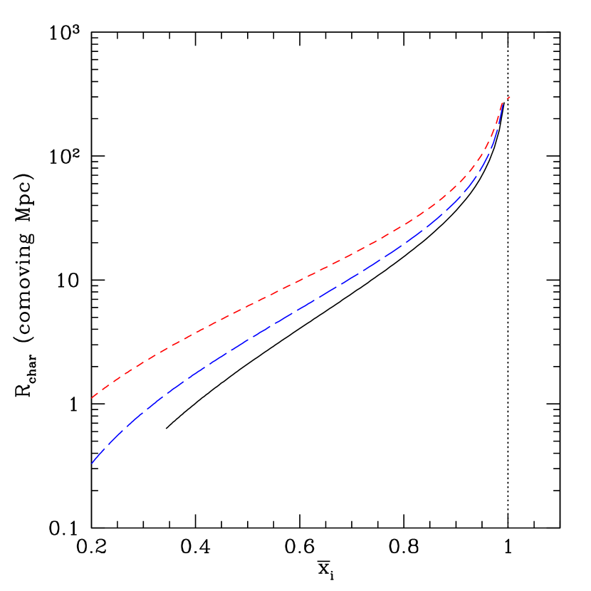
Figure 1.— Characteristic bubble radius (the peak of $Vdn/d{\rm log}R$) as a function of ionized fraction $\bar{x_{i}}(\zeta)$ for $z=6$ (solid), $z=9$ (long-dashed), and $z=15$ (short-dashed). The H II regions become quite large for $Q\gtrsim 0.5$, which justifies our approximation of uncorrelated bubbles at large $Q$. All of the reionization models considered in this paper are reionized well before $z=6$, so the upper two curves are most relevant.

We, therefore, are left with four integrals for the two bubble term $P_{2}$: two over mass and two over volume. The last two can be done analytically if we assume spherical symmetry for the bubbles and specify some condition for overlap. The most obvious choice is to disallow overlap, but, as mentioned, this leads to significant ringing. Another possibility, which we adopt here, is to enforce the following conditions: (1) $m_{1}$ cannot ionize $r_{2}$, and $m_{2}$ cannot ionize $r_{1}$; (2) the center of $m_{2}$ cannot lie inside $m_{1}$, but any other part of $m_{2}$ can touch $m_{1}$, and vice versa. To ensure that this scheme does not drastically overestimate $\langle x_{i}x_{i}^{\prime}\rangle$ near the bubble edges, we tune $\eta\sim.5$ in equation (17) to optimize agreement with the “exact” result—the correlation functions for the same model constructed explicitly from a Gaussian random field in a box of side-length $100h^{-1}$ Mpc using the method described in Zahn et al. (2005).

Figure 2 shows such a comparison for a model with $\zeta=40$. Our pseudo-analytic correlation functions are in excellent agreement with the exact result. If we had not allowed for some overlap or if we had set $\eta=1$ in our prescription for $\langle x_{i}~{}x_{i}^{\prime}\rangle$, the agreement would not be nearly as good. We do not expect perfect agreement because the exact correlation functions use a top hat filter in real space as opposed to the $k$-space filtering implicit in the extended Press-Schechter approach, which results in a slightly different bubble mass function (see §4.4 below).

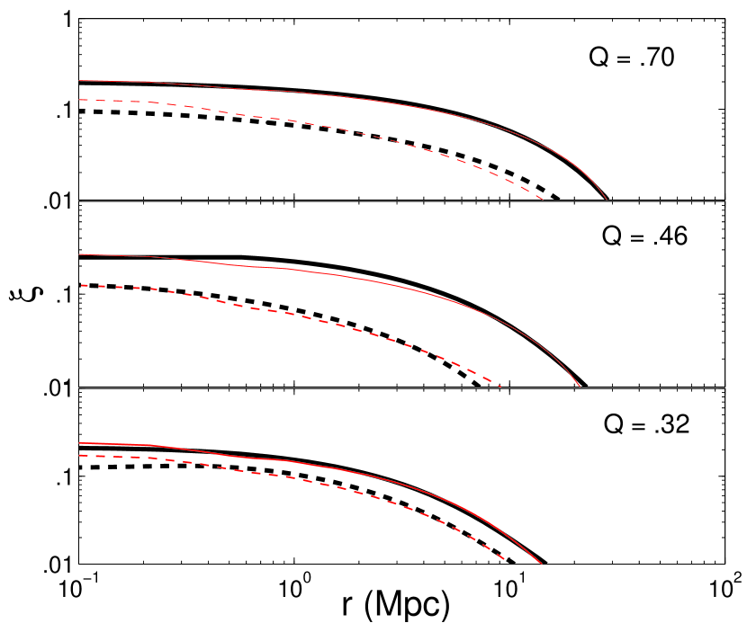
Figure 2.— Comparison of the analytic correlation functions in §3 (thick lines) with those calculated from a Gaussian random field in a box of side-length $100h^{-1}$ Mpc (thin lines), using the method described in Zahn et al. (2005). We compare these functions at three times during reionization for $\zeta=40$. The solid curves are $\xi_{xx}=\langle x_{i}\,x_{i}^{\prime}\rangle-\bar{x_{i}}^{2}$ and the dashed curves are $\xi_{x\,\delta^{\prime}}=\langle x_{i}\,\delta_{b}^{\prime}\rangle$. Note that the two methods are in good agreement. Although, we do not expect perfect agreement because the underlying mass function of the bubbles is slightly different for the two methods.

3.3. Cross-Correlation Between the Ionized Fraction and Density

Our prescription for $\langle x_{i}\,\delta_{b}^{\prime}\rangle$ is similar to $\langle x_{i}\,x_{i}^{\prime}\rangle$. We begin with the analog of equation (23) in FZH04

$$\langle x_{i}\delta_{b}\rangle(r) = -\bar{x}_{i}+\int dm_{h}\,\frac{m_{h}}{\bar{\rho}}\,n_{h}(m_{h})\int d^{3}{\bf r_{h}}u({\bf r}-{\bf r_{h}}|m_{h})$$ (20)

$$\times\,\int dm\,n(m)\int d^{3}{\bf r_{b}}[1+\xi_{bh}({\bf r_{h}-r_{b}})],$$

where $n_{h}$ is the dark matter halo number density, $u$ is the normalized halo profile (which we can approximate as a delta function because halos are much smaller than bubbles), and $\xi_{bh}$ is the excess probability of having a halo of mass $m_{h}$ at ${\bf r}_{h}$ given a bubble of mass $m$ at ${\bf r}_{b}$.

To evaluate equation (20), we break up the halos into those within the same bubble as the point ${\bf r}_{b}$ and those outside of it. If ${\bf r}_{h}$ resides inside the same bubble of mass $m$ as ${\bf r}_{b}$ then we know from §3.1 that $\xi_{bh,in}=n_{h}(m_{h}|m)/n_{h}(m_{h})-1$. The conditional mass function $n_{h}(m_{h}|m)$ can be computed using the extended Press-Schechter formalism (Furlanetto et al., 2004). Thus the contribution to equation (20) is

$$P_{\rm in}(r) = \int dm\,n(m)\,V_{0}(m,r)\int dm_{h}\frac{m_{h}}{\rho}\,n_{h}(m_{h}|m)$$ (21)

$$= \int dm\,n(m)\,V_{0}(m,r)\,[1+\delta_{B}].$$

In the last line, we use the fact that the inner integral is simply $1+\delta_{B}$, the mean overdensity of the bubble.

If ${\bf r_{h}}$ is outside the bubble containing ${\bf r_{b}}$, then we again use the trick $\xi_{bh}\approx b_{h}(m_{h})\,\bar{b}_{x}\,\xi_{\delta\delta}(r)$ (with the mean bias inserted for simplicity). Thus the contribution to the integral in equation (20) from outside the bubble is

$$P_{\rm out}(r) = \bar{x}_{i}-\int dm\,n(m)\,V_{0}(m,r)+\int dm\,n(m)$$ (22)

$$\times\,\int d^{3}{\bf r_{b}}\,[\bar{b}_{x}\,\xi_{\delta\delta}(r_{\rm eff})],$$

where the ${\bf r}_{b}$ integration is over all bubbles that ionize ${\bf r}_{b}$ but not ${\bf r}_{h}$ and, for simplicity, we evaluate $\xi_{\delta\,\delta}$ at separation $r_{\rm eff}={\rm max}[R(m),r]$ rather than at ${\bf r}-{\bf r}_{b}$. Note that the second term in $P_{\rm out}$ cancels the first term in $P_{\rm in}$. As before, the last term becomes problematic as $Q\rightarrow 1$; here, these difficulties arise primarily from our adoption of linear bias, which tends to overestimate the clustering in this limit. Fortunately, the term $P_{\rm out}$ is unimportant at large $Q$ because the effective bubble radius is quite large. So external clustering can be ignored and the one bubble term dominates. We again break our calculation into two parts:

$$\langle x_{i}\,\delta_{b}\rangle(r) =\left\{\begin{array}[]{l r}P_{\rm in}-P_{1}&Q>\eta^{\prime},\\ P_{\rm in}+P_{\rm out}-Q&{\rm otherwise},\end{array}\right.$$ (25)

where $P_{1}$ is given by equation (18). The solution $P_{\rm in}-P_{1}$ is an ansatz for when correlations with the density field inside the bubbles dominate $\langle x_{i}\,\delta_{b}^{\prime}\rangle$, which happens when the bubbles become large. We tune $\eta^{\prime}$ to get the best agreement with the “exact” $\langle x_{i}\,\delta_{b}^{\prime}\rangle$; this turns out to be when $\eta^{\prime}\sim.5$. Figure 2 compares our expression for $\langle x_{i}\,\delta_{b}^{\prime}\rangle$ with the “exact” result. We see that we are in good agreement. Because we smooth the density field on the scale of the bubbles and do not include the effects of non-sphericity, we should underpredict some of the small scale power. This underestimate appears to be very minor, affecting smaller scales than are relevant to our kSZ calculation.

4. The kSZ Effect from Reionization

4.1. Single Reionization Episodes

In the simplest scenario for reionization, a single generation of sources, such as population II stars, ionizes the universe. At each redshift, the ionized fraction equals the collapsed fraction times $\zeta$ (§3). We calculate the kSZ power spectrum for models with $\zeta$ =12, 40, and 500, which produce total optical depths of $\tau=0.085$, $0.117$, and $0.184$, respectively (assuming that helium is singly ionized along with hydrogen during reionization and is fully ionized by $z=3$; c.f. Sokasian et al. 2002). In addition, to investigate the effect of a longer reionization epoch on the kSZ signal, we calculate the power spectrum for a model where $\zeta$ increases linearly with redshift from $\zeta=40$ when reionization is complete ($z\sim 11$) to $\zeta=300$ at the start of reionization ($z\sim 22$). This model yields an optical depth of $\tau=0.138$. Physically, a monotonically increasing $\zeta(z)$ could happen if lower mass halos have larger escape fractions. The optical depths produced by all four models are within 2-$\sigma$ of the WMAP best fit value of $\tau=0.17\pm.04$ (Kogut et al., 2003). Figure 3 plots $Q(z)$ for the four single reionization models.

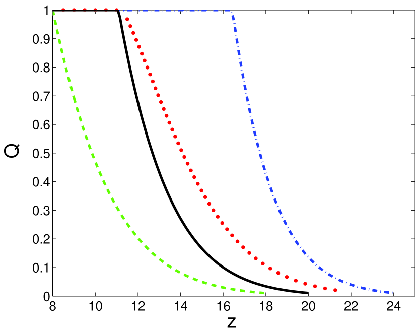
Figure 3.— Evolution of the global ionized fraction for single reionization models with $\zeta=12$, $40$, and $500$ (dashed, solid and dot-dashed, respectively). The dotted curve assumes that $\zeta$ evolves linearly with redshift from $\zeta=40$ at $z\sim 11$ to $\zeta=300$ at the start of reionization ($z\sim 22$).

Figure 4 shows the various contributions to the high-l kSZ power spectrum for the $\zeta=40$ model. The medium-width solid line is the total ${\it l}^{2}C_{\it l}/{2\pi}$ from patchy reionization – the sum of the contributions in equation (6) that depend on $P_{\delta_{x}\delta_{x}}$ (dashed) and $P_{\delta_{x}\delta_{b}}$ (dot-dashed). The contribution from $P_{\delta_{x}\delta_{x}}$ is larger than the cross correlation $P_{\delta_{x}\delta_{b}}$ at all scales, but the latter is never negligible. The dotted line is the OV power spectrum, which is larger than the patchy signal. The bulk of the OV effect comes from scattering off halos at times well after reionization, and it is therefore not optimal for studying the reionization epoch. In addition, we show the total high-l CMB power spectrum, comprised of both the lensed primordial anisotropies and the kSZ contributions (thick solid). Patchy reionization produces a larger kSZ signal than a uniform reionization scenario [$x_{i}({\bf x},z)=\bar{x}_{i}(z)$] with the same global reionization history; for comparison, we plot in Figure 4 the power spectrum for uniform reionization with the same $\bar{x}_{i}$ as $\zeta=40$ (thin solid).

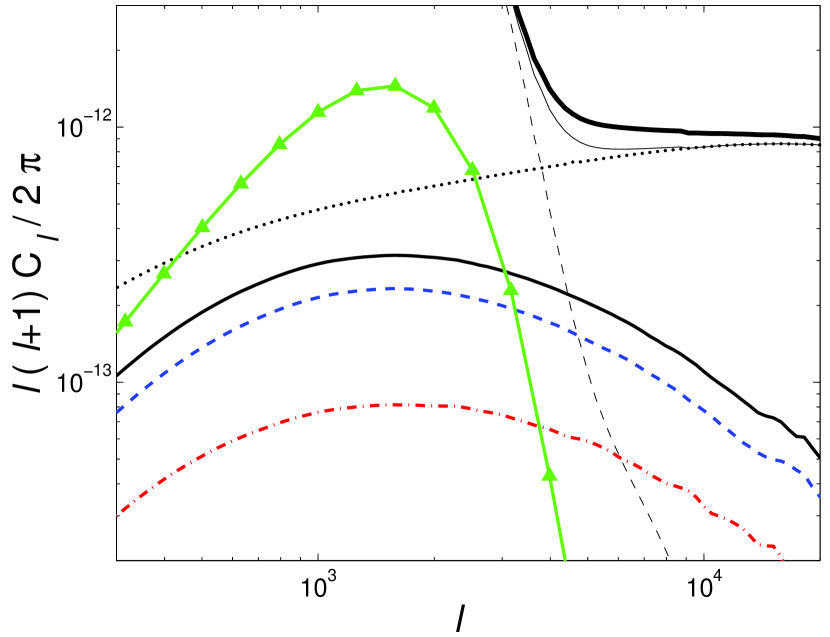
Figure 4.— Contributions to the power spectrum for $\zeta=40$. The three curves with the smallest amplitude are the patchy contributions from $P_{\delta_{x}\delta_{b}}$ (dot-dashed), $P_{\delta_{x}\delta_{x}}$ (dashed), and their total (solid). At larger amplitudes are the OV signal (dotted), the signal from the lensed primordial anisotropies (thin dashed), and the total power (thick solid). In addition, we show the total signal for a uniformly ionized medium (thin solid) and the patchy signal for the Gruzinov & Hu (1998) toy model with effective bubble size $R=10$ Mpc (solid with triangles). Both have the same $Q(z)$ as in the $\zeta=40$ model.

Gruzinov & Hu (1998) calculated the patchy signal for a simple and popular toy model where $\langle x_{i}({\bf x})~{}x_{i}({\bf x^{\prime}})\rangle=e^{-({\bf x}-{\bf x^{\prime}})^{2}/{2\,R^{2}}}(\bar{x}_{i}-{\bar{x}_{i}}^{2})+{\bar{x}_{i}}^{2}$ and where the cross correlation contribution is ignored. The discussion in §3 shows that the assumption of a Gaussian correlation function with constant standard deviation $R$ (the effective bubble size) throughout reionization is unrealistic. In our model, $\langle x_{i}\,x^{\prime}_{i}\rangle(r)$ is functionally closer to a decaying exponential than a Gaussian owing to the distribution of bubble sizes, and the shape of $\langle x_{i}\,x^{\prime}_{i}\rangle(r)$ evolves considerably during reionization as the bubbles grow and merge. Assuming a constant size results in a larger peak ${\it l}^{2}C_{\it l}/{2\pi}$ with the signal more concentrated at the specific scale. To illustrate this point, we plot the Gruzinov & Hu (1998) results for $R=10\mbox{ Mpc}$ and the same ionization history as our $\zeta=40$ model in Figure 4 (solid with triangles).

Figure 5 shows the patchy signal for the four single reionization models. Interestingly, this power differs by less than a factor of two between the curves. The slight differences in the amplitude owe mainly to the increase in density with redshift (the probability for scattering goes as $[1+z]^{3/2}$). This effect is partially cancelled because the universe ionizes over a somewhat shorter redshift interval as $\zeta$ increases. Of the four patchy curves in Figure 5, the evolving-$\zeta$ model has the largest amplitude, which reflects a general theme in our results: the amplitude of the patchy signal depends strongly on the duration of reionization. Finally, note that the OV contribution to the total power is larger than that of the patchy terms (see Figures 5 and 6). However, the relative differences between the OV contributions are comparable to the relative differences between the patchy contributions. Furthermore, most of the differences between the OV signals stem from these models fully ionizing at different times and not from differences in the duration of the reionization epoch.

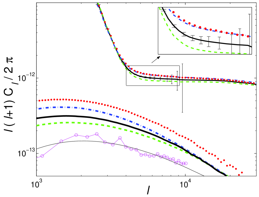
Figure 5.— Makeup of the high-l signal after removal of the tSZ anisotropies. We plot the patchy signal (thick) and total signal (thin) for $\zeta=12$ (dashed), $40$ (solid), and $500$ (dot-dashed), as well as a model with variable $\zeta$ (dotted). We include the 1-$\sigma$ error bars for ACT assuming perfect removal of point sources and the tSZ signal. We also plot the kSZ power from the simulation of Zahn et al. (2005) (circles) and compare this to our analytic model for a comparable $Q(z)$ (thin solid). We do not expect perfect agreement with the simulation because the bubble size distribution is slightly different.

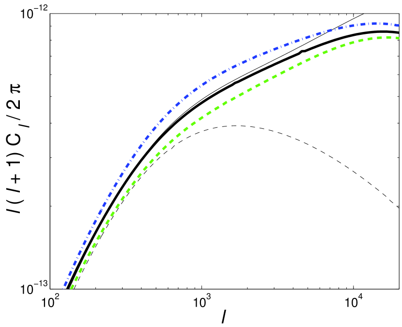
Figure 6.— The OV contribution to the signal for three of the single reionization models: $\zeta=12$ (dashed), $40$ (solid), and $500$ (dot-dashed). We also plot the OV signal for $\zeta=40$ in the extreme cases where the gas traces the dark matter distribution at all redshifts (thin solid) and with the linear theory density field (thin dashed).

At the bottom of Figure 5, we compare the patchy signal predicted by our analytic model to the kSZ power computed from a $100h^{-1}$ Mpc simulation of Zahn et al. (2005) (their model B). That paper uses the same model for the patchy epoch, as outlined in §3, imposed on an SPH simulation by directly applying the excursion set formalism to the density field of the box. The advantages to this approach are that it can allow for non-spherical bubbles and includes fully nonlinear bias for the bubbles. In addition, the simulation should more accurately account for nonlinearities in the density field. The disadvantages are that simulations encounter sample variance issues at large scales and offer less direct physical insight into the results. The patchy signal from the simulation agrees well with our analytic prediction for a comparable $Q(z)$, further justifying our simplifications in §2 and 3.

The ionization histories for the L20 and S5 simulations of Salvaterra et al. (2005) are similar to the single reionization histories discussed in this section. The authors find that the functional form and amplitude of the patchy signal for both models is similar, despite reionization ending earlier in the L20 model. This conclusion mirrors what we find here: the patchy signal is mostly affected by the duration of reionization and not by when reionization happens. Also, the peak amplitude of their patchy signal ($\approx 1.6\times 10^{-13}$ for both models) is comparable to what we find. Despite these similarities, Salvaterra et al. (2005) note that their $20h^{-1}$ Mpc simulation box may suppress the largest bubbles (particularly at the sizes predicted by our model). Such a bias would reduce the signal at lower l. It may be that simulations must employ larger boxes to accurately predict the patchy signal.

Figure 5 also plots the total signal (kSZ effect plus lensed primordial anisotropies) for the four models (thick lines) as well as the 1-$\sigma$ error bars for the Atacama Cosmology Telescope (ACT) in the 225 GHz channel. The error bars suggest that ACT will be able to distinguish between three of the four single reionization scenarios. These errors were obtained from the ACT specifications of $1.1$ arcminute resolution and $2\ \mu{\rm K}$ sensitivity, assuming perfect removal of point sources and the tSZ effect. The error bars are reliable if the frequency dependence of point source contaminants can indeed be modeled accurately. However, Huffenberger & Seljak (2004) showed that there will be significant bias in the measurements of the kSZ signal if this is not the case. It is uncertain how well the properties of point source contaminants can be modeled on these small scales.

4.2. Extended Reionization

Recently, a number of theoretical models have attempted to reconcile the CMB and quasar data by postulating an early generation of sources with high ionizing efficiency (most often because they contain massive, metal free stars) along with a self-regulation mechanism that switches to normal star formation with a lower ionizing efficiency (e.g., Wyithe & Loeb 2003; Cen 2003; Haiman & Holder 2003; Sokasian et al. 2003, 2004). Such scenarios can cause a plateau in the ionized fraction or even “double” reionization, in which ionized phases bracket a mostly neutral period (although the latter possibility is unlikely; Furlanetto & Loeb 2005). We refer to such scenarios as “extended reionization” and treat them as described in Furlanetto et al. (2004a).

We model extended reionization with two generations of sources. At some specified redshift, the first generation of sources turns off. For example, if the first generation consisted of massive, metal-free stars, the natural self-regulation condition halts the formation of these stars when the metallicity in collapsed objects passes some threshold (Bromm et al., 2001a, 2003; Mackey et al., 2003) or when hard photons moderate H₂ cooling (e.g. Yoshida et al. 2003a, 2004). Another possibility is that photoheating halts structure formation in biased regions. In either case, feedback slows down the growth of H II regions by reducing the effective $\zeta$ in ionized bubbles. We will simplify these conditions by assuming an instantaneous transition at some redshift $z^{*}$. In reality, the transition must be smooth and extended (Furlanetto & Loeb, 2005), but for our purposes we need only force the reionization history to stall. Thus, in our model, the universe develops a patchwork of H II regions at $z^{*}$ that have not yet overlapped completely. The first generation imprints a set of ionized bubbles, within which most of the second generation sources grow (because both appear in the same overdense regions). The bubbles grow only slowly until the total number of ionizations from the second generation become comparable to that of the first; after this point the evolution approaches the normal behavior. One important consequence of such a treatment is that it “freezes” a scale into the bubbles for a long period of time (Furlanetto et al., 2004a). More realistic histories may allow the scale to vary smoothly even during the stalling phase.

Consider a region of mass $m$ with a first generation of sources described by $(\zeta_{1},m_{{\rm min},1})$, which turn off at redshift $z^{*}$, and a second generation of sources with $(\zeta_{2},m_{{\rm min},2})$. We set $m_{{\rm min},2}=m_{\rm min}$ – the mass at which atomic cooling becomes efficient. The total number of ionizations is simply the sum of ionizations from the two generations. The excursion set barrier $\delta_{x}(m)$ will be the solution of

$$1 = (\zeta_{1}-\zeta_{2})\,{\rm erfc}\left\{\frac{\delta_{c}-\delta_{x}(m)}{\sqrt{2[\sigma^{2}(m_{\rm min,1},z^{\prime})-\sigma^{2}(m,z^{\prime})]}}\right\}$$ (26)

$$+\,\zeta_{2}\,{\rm erfc}\left\{\frac{\delta_{c}-\delta_{x}(m)}{\sqrt{2[\sigma^{2}(m_{\rm min,2},z)-\sigma^{2}(m,z)]}}\right\},$$

where $z^{\prime}=z^{*}$ for $z<z^{*}$ and $z^{\prime}=z$ otherwise. Here, the complementary error functions are the fraction of collapsed gas above the mass thresholds at the two redshifts. With the new barrier, the formalism from §3 carries over without further modification (note that the barrier remains nearly linear). Of course, our prescription ignores the effect of recombinations. However, even a relatively small number of second generation ionizing sources should be enough to halt recombinations within the H II bubbles.

Figures 7 and 8 plot the ionization histories and angular power spectra for three extended reionization models whose parameters and optical depths are listed in Table 1. The first generation of sources turn off at $z^{*}=18$ when $\bar{x}_{i}\sim 0.5$ in models (I) and (II). However, the minimum mass is ten times smaller in model (II). This smaller minimum mass could arise from efficient molecular cooling within halos. Smaller minimum masses and smaller $\zeta_{1}$ both result in a somewhat smaller effective bubble radius $R_{\rm eff}$. Because the amplitude of the signal scales roughly as the effective bubble size $R_{\rm eff}$ (Gruzinov & Hu, 1998), the peak signal in model (II) is smaller than in model (I). However, at smaller scales, smaller bubbles cause (II) to have slightly more power than (I). In model (III), the first generation of sources terminates at a high redshift, when $\bar{x}_{i}\sim 0.15$. This results in a smaller signal than the other extended reionization scenarios but still significantly more than the models described in §4.1. The OV signals for the three double reionization models are nearly identical because the redshift of overlap is almost the same. As a result, the differences in the kSZ angular power spectra stem primarily from their patchy contributions.

Table 1Parameters and optical depths for the three extended reionization scenarios considered in this paper. The quantity $m_{\rm min}$ is the minimum mass at which atomic cooling becomes efficient.

Model	$\zeta_{1}$	$\zeta_{2}$	$m_{\rm min,2}$	$z^{*}$	$\tau$
(I)	12	500	$m_{\rm min}$	18	0.144
(II)	12	100	$0.1\times m_{\rm min}$	18	0.151
(III)	12	500	$m_{\rm min}$	20	0.108

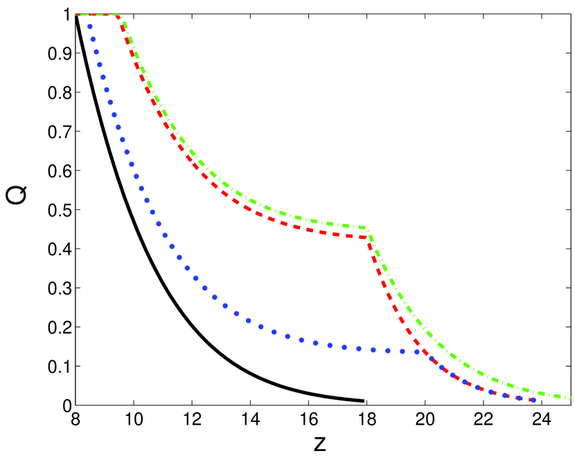
Figure 7.— Evolution the global ionized fraction for the three extended reionization models in Table 1. Model (I) is dashed, (II) is dot-dashed, and (III) is dotted. We also plot the single reionization model with $\zeta=12$ (solid) for comparison.

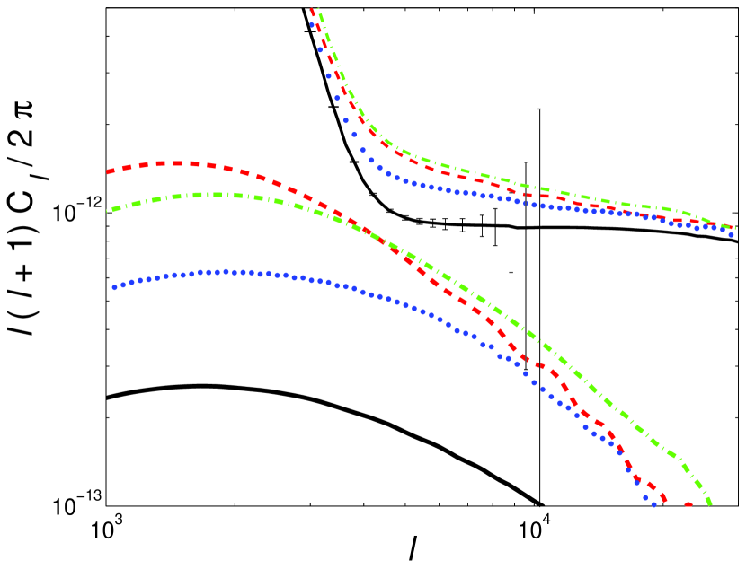
Figure 8.— Thick curves show the power spectrum from patchy reionization and the thin curves show the total power spectrum of the CMB once the tSZ anisotropies are removed. The solid curves are for $\zeta=12$ and the dashed, dot-dashed, and dotted curves are for the extended reionization models (I), (II) and (III), respectively. We include the 1-$\sigma$ ACT error bars.

All three extended reionization models result in substantially more signal at the relevant scales than the single ionization case $\zeta=12$ (see Fig. 8). This should allow future experiments to distinguish between these two sets of scenarios relatively easily. The reionization models considered in Santos et al. (2003) are most similar to the extended scenarios considered in this section. They find that the kSZ signal peaks around ${\it l}_{\rm peak}\sim 2000$ with an amplitude ${\it l}^{2}C_{l}/{2\pi}\sim 2\times 10^{-12}$. This ${\it l}_{\rm peak}$ is at a similar location in our extended models, and the amplitude is a bit larger than ours. However, our signal falls off more rapidly than theirs for ${\it l}>{\it l}_{\rm peak}$.

We note that our simplified treatment of extended reionization, with an instantaneous transition and few recombinations, may affect some aspects of these results. However, the large amplitude of the patchy component depends primarily on the duration over which the patchiness persists and depends only weakly on our model’s roughly constant characteristic scale during this period. Allowing the bubble size to evolve throughout the stalling phase will tend to flatten the power spectrum but will not substantially reduce the overall power.

4.3. Uniform Reionization

On the scale of our bubbles, even a neutral universe is optically thin to X-rays and gamma rays. If sources emit a large fraction of their energy in high energy photons (Oh, 2001; Venkatesan et al., 2001; Ricotti & Ostriker, 2003; Madau et al., 2004) or if there is a particle that decays into high energy photons at high redshifts (Sciama, 1982; Hansen & Haiman, 2004), such photons could ionize the universe more or less uniformly.

First, consider a scenario where a decaying particle uniformly ionizes the universe, which then recombines fully before stars turn on. In this case, only the OV power will be affected by the uniform component. However, the contribution to the OV signal from such high redshifts is negligible anyway. If, on the other hand, the epoch of uniform ionization overlaps with the patchy epoch, the net effect will be to decrease the amplitude of the patchy signal and increase the average bubble size. Both scenarios suggest that observations of the kSZ effect may be able to break the optical depth degeneracy between ionizations by a (uniform) decaying particle and discrete sources that would imprint a patchy signal. Alternatively, the ionizing sources could emit both ultraviolet and high energy photons so that the universe has both uniform and patchy components to the ionization field. This could occur if quasars or mini-quasars account for a significant fraction of the ionizing photons (but see Dijkstra et al. 2004 for limits on such a scenario).

To model this possibility, we suppose that the IGM has a uniform ionization fraction $\bar{x}_{u}(z)$. On top of this lie spatial variations from isolated H II regions. In this case, the condition $f_{\rm coll}>\zeta^{-1}(1-\bar{x}_{u})$ replaces the barrier in our model: each galaxy can produce a larger ionized bubble with the same number of ionizing photons. However, rather than varying from zero to unity, we have $0<x_{H}<(1-\bar{x}_{u})$. This damps the fluctuations from the bubbles, requiring the rescaling $\langle x_{i}x_{i}^{\prime}\rangle-\bar{x}_{i}^{2}\rightarrow(1-\bar{x}_{u})^{2}\,(\langle x_{i}x_{i}^{\prime}\rangle-\bar{x}_{i}^{2})$ and $\langle x_{i}\delta_{b}^{\prime}\rangle\rightarrow(1-\bar{x}_{u})\langle x_{i}\delta_{b}^{\prime}\rangle$ (this increases the importance of the cross-correlation term). Otherwise our formalism is unchanged.

In Figure 9, we plot reionization scenarios where the uniform component is proportional to the total ionized fraction, $\bar{x}_{u}=\mu\,\zeta\,f_{\rm coll}$ [it follows that the patchy fraction is $x_{p}=(1-\mu)\,\zeta\,f_{\rm coll}$]. We plot results for $\zeta=40$ with proportionality factors $\mu=0.0$ (solid), $\mu=0.25$ (dot-dashed), $\mu=0.5$ (dashed) and $\mu=1.0$ (thin solid). The rough interpretation is that $\mu$ parameterizes the fraction of ionizations caused by high energy photons emitted by discrete sources. The choice $\mu=0.0$ corresponds to normal patchy reionization and $\mu=1$ to purely uniform reionization. The ionized fraction $\bar{x}_{i}(z)$ is the same for all of these curves (the solid line in Figure 3). Note that the power spectrum for $\mu=0.25$ and $\mu=0.5$ is suppressed by a factor of $\sim 1.5$ and $\sim 3.0$ from the patchy model $\mu=0.0$. The 1-$\sigma$ error bars in Figure 9 suggest that ACT is capable of distinguishing between these models.

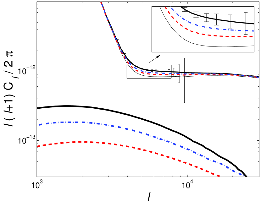
Figure 9.— Same as Figure 8, but with curves for $\zeta=40$ (solid) and for three uniform reionization scenarios with $\zeta=40\,(1-\mu)$ and $\bar{x}_{u}=40\,\mu\,{\it f}_{\rm coll}$. We show $\mu=0.25$ (dot-dashed), $\mu=0.5$ (dashed) and $\mu=1.0$ (thin solid). These models have the same $Q(z)$ as the canonical $\zeta=40$ model and therefore the same OV signal. We include the 1-$\sigma$ ACT error bars.

4.4. Reionization and Uncertainties in the Underlying Cosmology

Even though the least well-known parameter in our model is $\zeta$, there is enough uncertainty in the cosmological parameters and the mass function to strongly affect the morphology of reionization. Beyond the usual uncertainty in $\Omega_{m}$, $n$, etc., there is also the shape and amplitude of the mass function at high redshifts; each choice will yield a different reionization history. Simulations are our best avenue for ascertaining the correct mass function. However, to date most high-resolution simulations have only investigated epochs well after reionization. We found two studies of the mass function at $z\gtrsim 10$. Jang-Condell & Hernquist (2001) showed that the Press-Schechter mass function agrees reasonably well with the mass function from their simulation at $z=10$. However, their $1h^{-1}$ comoving Mpc cube only allowed them to probe the low-mass end. The other was Reed et al. (2003), which concludes that the Sheth & Tormen (2002) mass function overpredicts substantially the mass function in simulations for $z>10$. In Figure 10, we plot the expected reionization history $Q(z)$ for several mass functions: Sheth-Tormen (thick dashed), the usual Press-Schechter function (thick solid), and Press-Schechter with a top hat real space filter computed from random walks (thick dot-dashed). Surprisingly, the top hat real space filter gives a significantly smaller collapse fraction than the sharp $k$-space filter implicit in the extended Press-Schechter formalism (by about a factor of $0.5$). This is because the variance in the density field within the top hat window function is smaller than the variance within the sharp $k$-space window function. Since the barrier $\delta_{c}=1.686$ is derived from top hat considerations, it could well be that the top hat in real space gives a more realistic mass function at these high redshifts.

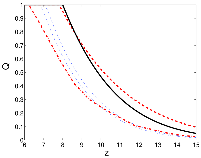
Figure 10.— Comparison of reionization histories with $\zeta=12$ between cosmologies that have different mass functions and cosmological parameters. The thick solid is the standard cosmology adopted in this paper with the Press-Schechter mass function. Other curves show the same model except for $\sigma_{8}=0.8$ (thin dot-dashed) and for tilt $n=0.95$ (thin dashed). We also plot the $Q(z)$ for the Sheth-Tormen mass function (thick dashed) and Press-Schechter with a top hat real space filter calculated from random walks (thick dot-dashed).

Several observations of large scale structure predict a lower value of $\sigma_{8}$ than the $\sigma_{8}=0.9$ from CMB data (Tegmark et al., 2004). We plot $Q(z)$ for $\sigma_{8}=0.8$ (but with other parameters fixed) in Figure 10 (thin dot-dashed). This value for $\sigma_{8}$ causes reionization to end later. In addition, CMB observations are consistent with the tilt $n$ in the primordial power spectrum being slightly less than the Harrison-Zel’dovich choice $n=1$ (Spergel et al., 2003; Tegmark et al., 2004). Even a slightly smaller tilt, $n=0.95$ (thin dashed), causes the universe to reionize significantly later.

Neither these different cosmological parameters nor a different mass function significantly alters the duration of reionization. Because the kSZ amplitude is most affected by the duration of reionization, all of the reionization histories in Figure 10 should produce similar patchy signals. However, the amplitude of the tSZ effect scales as $\sim\sigma_{8}^{6-9}$ (Seljak et al., 2001) and the OV signal scales as $\sim\sigma_{8}^{4-6}$ (Zhang et al., 2004). Thus, if $\sigma_{8}$ is smaller than $0.9$ these anisotropies will be suppressed, and the patchy signal will be more prominent.

If the dark matter is warm, this will have an even more drastic effect on the ionized fraction (Barkana et al., 2001; Kitano & Low, 2005). Warm dark matter will create a cutoff in the transfer function at small scales such that the collapsed fraction is significantly smaller. While warm dark matter cannot make universes with a high optical depth (Yoshida et al., 2003b), this can be supplemented by having a decaying particle ionize the universe at higher redshifts (Hansen & Haiman, 2004).

Finally, we note that because the OV effect is dominated by lower redshift structure formation, the uncertainty in the high-$z$ mass function has only a negligible effect on that signal.

5. Discussion

We find that there is a clear and measurable difference between the amplitude of the kSZ signal for models where Population II stars dominate reionization, where Population III stars are also important (or reionization is extended for some other reason), and where there are a large number of hard photons (or uniform reionization). At scales where the kSZ effect dominates over other primordial anisotropies, the amplitude of the patchy signal differs by as much as $10{\mu{\rm K}}^{2}$. Other aspects of the patchy signal also differ between reionization histories, such as the multipole ${\it l}$ where the patchy power spectrum peaks. The peak of the power spectrum is primarily determined by the distribution of bubble sizes when $Q\sim 0.5$ or, for our extended reionization scenarios, by the bubble size when the ionized fraction “freezes.” Ideally, one could fit a simple (but physically motivated) two or three parameter model to the observations. Of course, reionization is a very complex process and many parameters are needed to describe its morphology in detail (in our model, these are essentially the parameters determining $\zeta$ as a function of redshift). To add to the difficulty, observations cannot separate the OV and patchy contributions to the CMB power spectrum, requiring simultaneous fits to both. The OV power is dominated by post-reionization sources and contains much less information about the morphology of reionization than the patchy signal.

The OV contamination of the patchy signal might not be a problem. First, because a substantial fraction of the OV power comes from low redshift objects, much of it may be removable from the signal. Also, future 21cm observations will help separate these two contributions (e.g., FZH04, Furlanetto et al. 2004a; Salvaterra et al. 2005; Zaldarriaga et al. 2004). Furthermore, with a fixed cosmology, the OV contribution to the power spectrum is determined only by the distribution of gas. To zeroth order, we know that gas traces the dark matter distribution, which can be successfully modeled with halo theory. At large overdensities our understanding of the gas distribution is incomplete. But for ${\it l}<10^{4}$, the OV power is relatively independent of the gas distribution under reasonable assumptions. This is evident in Figure 6, where the thin black curve is the OV signal in the most extreme case in which the baryons trace the dark matter. Zhang et al. (2004) contend that one can reasonably calculate the OV contribution without any free parameters as long as the evolution of the ionized fraction is known. The ionized fraction at each redshift is a byproduct of the model for patchy reionization. Therefore, the OV signal – which has a much flatter power spectrum – is predicted by our model with no additional parameters (to lowest order) and could help break the degeneracy between the redshift of overlap and other parameters. Of course, minor differences do remain in the calculation of the OV signal between different computational approaches (see §2). We expect that future research, particularly simulations incorporating realistic gas heating, will help to resolve these small discrepancies.

To this point, we have concentrated on the information contained in the kSZ signal. However, it will also contaminate fits to the primordial anisotropies. Knox et al. (1998), Santos et al. (2003) and Zahn et al. (2005) investigated how the signal from patchy reionization will bias cosmological parameter determination for WMAP and Planck. While the net effect is insignificant for WMAP, it will be quite substantial for Planck, which can measure $C_{\it l}$ to ${\it l}=2500$. In this case, the bias for many cosmological parameters is comparable to the 1-$\sigma$ statistical error. Santos et al. (2003) propose adding an additional parameter, the effective amplitude of the kSZ power spectrum, in future fits to Planck data, which is justified by the fact that the kSZ signal is fairly flat in the regime where it affects the fit. A similar conclusion holds for our model for reionization (Zahn et al., 2005). The polarization-polarization CMB power spectrum might be more reliable for measuring the cosmological parameters at ${\it l}\gtrsim 1000$ since it is nearly unaffected by patchiness (Zahn et al., 2005).

Other probes of the reionization epoch may help to restrict the set of possible reionization histories, facilitating the interpretation of the kSZ signal measured by ACT or SPT. A more precise measurement of the optical depth $\tau$ from measurements of large-scale CMB polarization will significantly reduce the set of viable models. In addition, if future observations of high-redshift quasars or 21 cm emission from neutral hydrogen can pin down the redshift of overlap, this will again reduce the set of plausible models. To the extent that the current large optical depth measurement implies a long period of extended reionization, the patchy contribution should extend over a long redshift interval and have a substantial amplitude. This will allow future experiments to distinguish reionization by stellar sources, hard photons, and decaying particles, and alleviate many of the degeneracies from large-scale CMB polarization data alone.

Appendix A The Baryon Distribution

We construct $P_{\delta_{b}\delta_{b}}$ from the halo model by using NFW dark matter halo profiles with the Jenkins mass function and by setting $P_{\delta_{b}\delta_{b}}(k)=F(k/k_{F})^{2}\,P_{\delta\delta}(k)$, where $F(x)$ filters large $k$ modes in order to approximate the effects of finite gas pressure. The Jeans length is often not the appropriate filtering scale $k_{F}$. Gnedin & Hui (1998) and Gnedin (1998) suggest $k_{F}(z)=34\,\sqrt{\Omega_{m}(z)}h$ Mpc^-1 for thermal history-dependent filtering and

$$F(x)=\frac{1}{2}\left[e^{-x^{2}}+\frac{1}{{(1+4x^{2})}^{1/4}}\right].$$ (A1)

They find that for $\delta<10$, this filtering function produces errors smaller than $10\%$ in the gas power spectrum $P_{\delta_{b}\delta_{b}}$. We use this scheme for $z<8$ and set $F(x)=1$ for $z>8$, where the gas distribution is less well-understood and it is thought that cooling is more efficient. Note that the difference in the kSZ signal between reasonable filtering schemes for high redshifts is minute on the scales of interest.

Appendix B Configuration Space Calculation of the kSZ Effect

For the patchy terms, namely $\langle x_{i}\,x_{i}^{\prime}\rangle\langle v\,v^{\prime}\rangle$ and $\langle x_{i}\,\delta_{b}^{\prime}\rangle\langle v\,v^{\prime}\rangle$, we perform the kSZ calculation in configuration space using equation (3). We first use linear theory to construct the velocity field. In that case, the velocity correlation function is

$$\langle v(\eta,{\bf\hat{n}})\,v(\eta^{\prime},{\bf\hat{n}^{\prime}})\rangle=[\xi_{\perp}(r)]\,{\bf\hat{n}}\cdot{\bf\hat{n}^{\prime}}+[\xi_{||}(r)-\xi_{\perp}(r)]\,\frac{({\bf r}\cdot{\bf\hat{n}})({\bf r}\cdot{\bf\hat{n}^{\prime}})}{r^{2}},$$ (B1)

where $v({\bf\hat{n}})={\bf v}({\bf\hat{n}})\cdot{\bf\hat{n}}$, ${\bf r}\equiv{\bf x}-{\bf x^{\prime}}$ and $\xi_{||}$ and $\xi_{\perp}$ are the autocorrelation functions of the velocity parallel and perpendicular to ${\bf r}$:

$$\binom{\xi_{||}}{\xi_{\perp}}=-{\it f}^{2}H_{0}^{2}\int_{0}^{\infty}\frac{dk}{2\pi^{2}k}P_{\rm lin}(k)\binom{j_{0}^{\prime}(kx)/x}{k~{}j_{0}^{\prime\prime}(kx)}.$$ (B2)

Here primes denote derivatives with respect to $kx$. If we put the correlation functions constructed here and in §3 into equation (3), we can calculate $w(\theta)$ directly. For ${\it l}\gg 1$, the angular power spectrum is then

$$C_{\it l}\approx 2\pi\int_{0}^{\infty}\theta d\theta\,J_{0}({\it l}\theta)\,w(\theta).$$ (B3)

Appendix C Derivation of $Q(z)$ and Mass Function for a Linear Barrier

Our aim in this section is to derive (or rederive) some relations we will need for a linear barrier using the extended Press-Schechter formalism (Bond et al., 1991; Lacey & Cole, 1993). The advantage of this approach is that the probability distribution of $\delta_{k}$ – the real-space density within a $k$-space top hat filter of radius $k$ – becomes the solution to a diffusion equation. This diffusion equation can then be solved for various boundary conditions (corresponding to the specified barrier). We first rederive the familiar result for a constant barrier adopting the notation of Scannapieco & Barkana (2002) and then expand the approach to the case of a linear barrier. The variance today in a region defined by a sharp $k$-space window function is

$$S_{k}=\sigma^{2}(k)=\frac{1}{2\pi^{2}}\int_{0}^{k}dkk^{2}P_{\rm lin}(k),$$ (C1)

where $P_{\rm lin}(k)$ is the linear power spectrum at $z=0$. As we change the smoothing scale – or increase $k$ in equation (C1) – each step $\Delta S_{k}$ is uncorrelated with the previous $S_{k}$ (this is not true for other filter choices). Therefore, we can write a simple evolution equation for $Q(\delta,S_{k})$, the probability distribution for the density field at smoothing scale $k$ (Bond et al., 1991)

$$Q(\delta,S_{k})=\frac{1}{\sqrt{2\pi\,{\Delta S_{k}}}}\int_{-\infty}^{\infty}{d\Delta\delta\,{\rm exp}\left[-\frac{(\Delta\delta)^{2}}{2\,{\Delta S_{k}}}\right]\,Q(\delta-\Delta\delta,S_{k}-\Delta S_{k})}.$$ (C2)

If we expand $Q$ to second order in $\Delta\delta$ and perform the $\Delta\delta$ integral, equation (C2) reduces to

$$Q(\delta,S_{k})=Q(\delta,S_{k}-\Delta S_{k})+\frac{1}{2}\frac{\partial^{2}Q(\delta,S_{k}-\Delta S_{k})}{\partial\delta^{2}}\,\Delta S_{k},$$ (C3)

noting that $\langle\Delta\delta\rangle=0$ and that $\langle(\Delta\delta)^{2}\rangle=\Delta S_{k}$. Rearranging the above equation and keeping terms to linear order in $\Delta S_{k}$ gives a diffusion equation

$$\frac{\partial Q(\delta,S_{k})}{\partial S_{k}}=\frac{1}{2}\frac{\partial^{2}Q(\delta,S_{k})}{\partial\delta^{2}}.$$ (C4)

In the absence of any barrier, the solution to this equation is

$$Q_{0}(\delta,S_{k})=\frac{1}{\sqrt{2\pi\,S_{k}}}{\rm exp}\left[-\frac{\delta^{2}}{2\,{S_{k}}}\right].$$ (C5)

The solution to a diffusion equation is uniquely specified by the initial and boundary conditions. Thus, for a constant barrier $B(k)=B_{0}$, we can guess the unique solution that satisfies the boundary condition $Q(B_{0},S)=0$, namely $Q=Q_{0}(\delta,S_{k})-Q_{0}(2B_{0}-\delta,S_{k})$. The second term is an “image” that is placed to cancel the contribution of the source term on the boundary (Chandrasekhar, 1943; Bond et al., 1991).

For the bubble problem, we are ultimately interested in a solution to this diffusion equation for a barrier that is linear in the variance $B(k)=B_{0}+B_{1}S_{k}$. This amounts to the boundary condition $Q(B(k),S_{k})=0$ for the PDE (C4). To find a solution, let us rescale the variable $\delta$ to $y=B_{1}(\delta-B_{1}S_{k})$ such that the diffusion equation transforms to

$$\frac{\partial Q}{\partial S_{k}}=\frac{B_{1}^{2}}{2}\left[\frac{\partial^{2}Q}{\partial y^{2}}+2\,\frac{\partial Q}{\partial y}\right],$$ (C6)

and the boundary condition becomes $Q(B_{1}\,B_{0},S_{k})=0$. Unlike the constant barrier problem, the image method is not a fruitful way to solve this problem. Instead, let us look for solutions of the form $Q(y,S_{k})=g(y)\,f(S_{k})$. Then equation (C6) becomes

$$\frac{1}{f}\frac{\partial f}{\partial S_{k}}=\frac{B_{1}^{2}}{2\,g}\left[\frac{\partial^{2}g}{\partial y^{2}}+2\,\frac{\partial g}{\partial y}\right]=\lambda.$$ (C7)

Dropping constant factors, the general solutions for $f$ and $g$ are $f(S_{k})={\rm exp}(\lambda\,S_{k})$ and $g(y)={\rm exp}[(-1\pm{\it i}X)\,y]$ where $X=-{\it i}\sqrt{1+2\lambda/B_{1}^{2}}$. If we drop the eigenfunctions which do not satisfy the boundary conditions, our solution $Q(y,S_{k})$ becomes

$$Q_{\rm lb}(y,S_{k})=\int_{0}^{\infty}{dX}h(X)~{}{\rm sin}[X(y-B_{0}B_{1})]~{}\exp\left[-y-\frac{B_{1}^{2}}{2}(1+X^{2})S_{k}\right].$$ (C8)

To determine $h(X)$, we impose the initial condition. In the $(\delta,S)$ coordinates, the initial condition is $\delta_{D}(\delta)\equiv{\rm lim}_{S_{k}\rightarrow 0}\,{\rm exp}[-\delta^{2}/(2\,{S_{k}})]/\sqrt{2\pi\,S_{k}}$. If we substitute $y$ for $\delta$ this becomes ${\rm lim}_{S_{k}\rightarrow 0}\,{\rm exp}[{-B_{1}^{2}\,S_{k}/2-y-y^{2}/(2B_{1}^{2}S_{k})}]/\sqrt{2\pi S_{k}}=B_{1}\,\delta_{D}(y)\,{\rm exp}(-y)$. Using this, we find that $h(X)=B_{1}/\pi~{}{\rm sin}(XB_{0}B_{1})$, and we can now integrate equation (C8):

$$Q_{\rm lb}(y,S_{k}) = \frac{1}{\sqrt{2\pi S_{k}}}\,{\rm exp}{[-\frac{B_{1}^{2}S_{k}}{2}-y]}\left\{\exp\left[-\frac{y^{2}}{2B_{1}^{2}S_{k}}\right]-\exp\left[-\frac{(y-2B_{0}B_{1})^{2}}{2B_{1}^{2}S_{k}}\right]\right\}$$ (C9)

$$= \frac{1}{\sqrt{2\pi S_{k}}}\left\{\exp\left[-\frac{\delta^{2}}{2\,S_{k}}\right]-\exp\left[-\frac{|2(B_{0}+{\it i}\sqrt{B_{0}B_{1}S_{k}})-\delta|^{2}}{2S_{k}}\right]\right\}.$$ (C10)

The solution (C9) vanishes at the boundary $y=B_{0}B_{1}$, as required. In addition, equation (C10) shows that there is an analogous form to the familiar “image” decomposition for the constant barrier problem.

To obtain the ionized fraction, we integrate over all possible $\delta$ at $S_{k}=\sigma_{\rm min}^{2}$, which yields equation (11). We can obtain the mass function as well. The probability that a trajectory crosses the barrier in the interval $S_{k}$ to $S_{k}+dS_{k}$ is

$$P(S_{k})=-\frac{d}{dS_{k}}\int_{-\infty}^{B_{0}B_{1}}\left(\frac{dy}{B_{1}}\right)~{}Q_{\rm lb}=-\left[\frac{B_{1}}{2}\frac{\partial Q_{\rm lb}}{\partial y}\right]_{-\infty}^{B_{0}B_{1}}=\frac{B_{0}}{\sqrt{2\pi\,S_{k}^{3}}}{\rm exp}\left[-\frac{B(k)^{2}}{2\,{S_{k}}}\right],$$ (C11)

where the second inequality uses the diffusion equation and the boundary condition $Q_{\rm lb}(B_{0}B_{1},S_{k})=0$. Equation (C11) agrees with the results of Sheth (1998), which were derived through a different method. The number density of bubbles of mass $m$ is then $n(m)=\rho_{0}/m\,P(S_{k})\,|{{\rm d}S_{k}}/{{\rm d}m}|$, which yields equation (10).

References

- Aghanim, N., et al. (2001) Aghanim, N., Desert, F.X., Puget, J. L. & Gispert, R. 1996, A&A, 311, 1
- Arons & Wingert (1972) Arons, J. & Wingert, D. W. 1972, ApJ, 177, 1
- Barkana & Loeb (2001) Barkana, R. & Loeb, A. 2001, Phys. Rep., 349, 125
- Barkana et al. (2001) Barkana, R., Haiman, Z., & Ostriker, J. P. 2001, ApJ, 558, 482
- Becker et al. (2001) Becker, R. H. et al. 2001, AJ, 122, 2850
- Bond et al. (1991) Bond, J. R., Cole, S., Efstathiou, G., & Kaiser, N. 1991, ApJ, 379, 440
- Bromm et al. (2001a) Bromm, V., Ferrara, A., Coppi, P. S., & Larson, R. B. 2001a, MNRAS, 328, 969
- Bromm et al. (2001b) Bromm, V., Kudritzki, R. P., & Loeb, A. 2001b, ApJ, 552, 464
- Bromm et al. (2003) Bromm, V., Yoshida, N., & Hernquist, L. 2003, ApJ, 596, L135
- Cen (2003) Cen, R. 2003, ApJ, 591, L5
- Chandrasekhar (1943) Chandrasekhar, S. 1943, Reviews of Modern Physics, 15, 1
- Ciardi et al. (2003) Ciardi, B., Stoehr, F., & White, S. D. M. 2003, MNRAS, 343, 1101
- Cooray & Chen (2002) Cooray, A. & Chen, X. 2002, ApJ, 573, 43
- Cooray & Sheth (2002) Cooray, A. & Sheth, R. 2002, Phys. Rep., 372, 1
- da Silva et al. (2001) da Silva, A. C. et al. 2001, ApJ, 561, L15
- Dijkstra et al. (2004) Dijkstra, M., Haiman, Z., & Loeb, A. 2004, ApJ, 613, 646
- Dodelson & Jubas (1993) Dodelson, S. & Jubas, J. M. 1993, Physical Review Letters, 70, 2224
- Fan et al. (2002) Fan, X. et al. 2002, AJ, 123, 1247
- Furlanetto et al. (2004) Furlanetto, S. R., Hernquist, L., & Zaldarriaga, M. 2004c, MNRAS, 354, 695
- Furlanetto et al. (2004a) Furlanetto, S. R., Zaldarriaga, M., & Hernquist, L. 2004a, ApJ, 613, 16
- Furlanetto et al. (2004b) —. 2004b, ApJ, 613, 1 [FZH04]
- Furlanetto et al. (2004d) Furlanetto, S. R., Sokasian, A., & Hernquist, L. 2004d, MNRAS, 347, 187
- Furlanetto & Loeb (2005) Furlanetto, S. R. & Loeb, A. 2005, ApJ, in press (astro-ph/0409656)
- Gnedin (1998) Gnedin, N. Y. 1998, MNRAS, 299, 392
- Gnedin & Hui (1998) Gnedin, N. Y. & Hui, L. 1998, MNRAS, 296, 44
- Gruzinov & Hu (1998) Gruzinov, A. & Hu, W. 1998, ApJ, 508, 435
- Gunn & Peterson (1965) Gunn, J. E. & Peterson, B. A. 1965, ApJ, 142, 1633
- Haiman & Holder (2003) Haiman, Z. & Holder, G. P. 2003, ApJ, 595, 1
- Hansen & Haiman (2004) Hansen, S. H. & Haiman, Z. 2004, ApJ, 600, 26
- Hernquist & Springel (2003) Hernquist, L. & Springel, V. 2003, MNRAS, 341, 1253
- Hu (2000) Hu, W. 2000, ApJ, 529, 12
- Huffenberger & Seljak (2004) Huffenberger, K. M. & Seljak, U. 2004, New Astronomy, submitted, (astro-ph/0408066)
- Jaffe & Kamionkowski (1998) Jaffe, A. H. & Kamionkowski, M. 1998, Phys. Rev. D, 58, 043001
- Jang-Condell & Hernquist (2001) Jang-Condell, H. & Hernquist, L. 2001, ApJ, 548, 68
- Jenkins et al. (2001) Jenkins, A. et al. 2001, MNRAS, 321, 372
- Kaiser (1992) Kaiser, N. 1992, ApJ, 388, 272
- Kitano & Low (2005) Kitano, R. & Low, I. 2005 (hep-ph/0503112)
- Knox et al. (1998) Knox, L., Scoccimarro, R., & Dodelson, S. 1998, Physical Review Letters, 81, 2004
- Kogut et al. (2003) Kogut, A. et al. 2003, ApJS, 148, 161
- Lacey & Cole (1993) Lacey, C. & Cole, S. 1993, MNRAS, 262, 627
- Ma & Fry (2002) Ma, C. & Fry, J. N. 2002, Physical Review Letters, 88, 211301
- Mackey et al. (2003) Mackey, J., Bromm, V., & Hernquist, L. 2003, ApJ, 586, 1
- Madau et al. (2004) Madau, P. et al. 2004, ApJ, 604, 484
- Mesinger & Haiman (2004) Mesinger, A. & Haiman, Z. 2004, ApJ, 611, L69
- Mo & White (1996) Mo, H. J. & White, S. D. M. 1996, MNRAS, 282, 347
- Molnar & Birkinshaw (2000) Molnar, S. M. & Birkinshaw, M. 2000, ApJ, 537, 542
- Oh (2001) Oh, S. P. 2001, ApJ, 553, 499
- Oh & Furlanetto (2005) Oh, S. P. & Furlanetto, S. R. 2005, ApJ, 620, L9
- Ostriker & Vishniac (1986) Ostriker, J. P. & Vishniac, E. T. 1986, ApJ, 306, L51
- Press & Schechter (1974) Press, W. H. & Schechter, P. 1974, ApJ, 187, 425
- Reed et al. (2003) Reed, D. et al. 2003, MNRAS, 346, 565
- Ricotti & Ostriker (2003) Ricotti, M. & Ostriker, J. P. 2003, MNRAS, 352, 547
- Salvaterra et al. (2005) Salvaterra, R. et al. 2005, astro-ph/0502419
- Santos et al. (2003) Santos, M. G. et al. 2003, ApJ, 598, 756
- Scannapieco & Barkana (2002) Scannapieco, E. & Barkana, R. 2002, ApJ, 571, 585
- Sciama (1982) Sciama, D. W. 1982, MNRAS, 198, 1P
- Seljak et al. (2001) Seljak, U., Burwell, J., & Pen, U. 2001, Phys. Rev. D, 63, 063001
- Sheth (1998) Sheth, R. K. 1998, MNRAS, 300, 1057
- Sheth & Tormen (2002) Sheth, R. K. & Tormen, G. 2002, MNRAS, 329, 61
- Sokasian et al. (2002) Sokasian, A., Abel, T., & Hernquist, L. 2002, MNRAS, 332, 601
- Sokasian et al. (2003) Sokasian, A., Abel, T., Hernquist, L., & Springel, V. 2003, MNRAS, 344, 607
- Sokasian et al. (2004) Sokasian, A. et al. 2004, MNRAS, 350, 47
- Spergel et al. (2003) Spergel, D. N. et al. 2003, ApJS, 148, 175
- Springel & Hernquist (2003) Springel, V. & Hernquist, L. 2003, MNRAS, 339, 312
- Sunyaev & Zel’dovich (1980) Sunyaev, R. A. & Zel’dovich, I. B. 1980, MNRAS, 190, 413
- Tegmark et al. (2004) Tegmark, M. et al. 2004, Phys. Rev. D, 69, 103501
- Valageas et al. (2001) Valageas, P., Balbi, A., & Silk, J. 2001, A&A, 367, 1
- Venkatesan et al. (2001) Venkatesan, A., Giroux, M. L., & Shull, J. M. 2001, ApJ, 563, 1
- White et al. (2002) White, M., Hernquist, L., & Springel, V. 2002, ApJ, 579, 16
- White et al. (2003) White, R. L., Becker, R. H., Fan, X., & Strauss, M. A. 2003, AJ, 126, 1
- Wyithe & Loeb (2003) Wyithe, J. S. B. & Loeb, A. 2003, ApJ, 586, 693
- Wyithe & Loeb (2004) —. 2004, Nature, 427, 815
- Yoshida et al. (2003a) Yoshida, N., Abel, T., Hernquist, L. & Sugiyama, N. 2003a, ApJ, 592, 645
- Yoshida et al. (2003b) Yoshida, N., Sokasian, A., Springel, V. & Hernquist, L. 2003b, ApJ, 591, L1
- Yoshida et al. (2004) Yoshida, N., Bromm, V. & Hernquist, L. 2004, ApJ, 605, 579
- Zahn et al. (2005) Zahn, O., Zaldarriaga, M., Hernquist, L., & McQuinn, M. 2005, ApJ, submitted, (astro-ph/0503166)
- Zaldarriaga et al. (2004) Zaldarriaga, M., Furlanetto, S. R., & Hernquist, L. 2004, ApJ, 608, 622
- Zel’dovich & Sunyaev (1969) Zel’dovich, I. B. & Sunyaev, R. A. 1969, Astrophys. Space Sci., 4
- Zhang et al. (2004) Zhang, P., Pen, U., & Trac, H. 2004, MNRAS, 347, 1224