POINT-AGAPE Pixel Lensing Survey of M31 :
Evidence for a MACHO contribution to Galactic Halos

The POINT-AGAPE collaboration is carrying out a search for gravitational microlensing toward M31 to reveal galactic dark matter in the form of MACHOs (Massive Astrophysical Compact Halo Objects) in the halos of the Milky Way and M31. A high-threshold analysis of 3 years of data yields 6 bright, short–duration microlensing events, which are confronted to a simulation of the observations and the analysis. The observed signal is much larger than expected from self lensing alone and we conclude, at the 95% confidence level, that at least 20% of the halo mass in the direction of M31 must be in the form of MACHOs if their average mass lies in the range 0.5-1 M_⊙. This lower bound drops to 8% for MACHOs with masses $\sim 0.01$ M_⊙. In addition, we discuss a likely binary microlensing candidate with caustic crossing. Its location, some 32’ away from the centre of M31, supports our conclusion that we are detecting a MACHO signal in the direction of M31.

1 Introduction

Gravitational microlensing, as first noted by Paczyński (1986), is a powerful tool for the detection of massive astrophysical halo compact objects (MACHOs), a possible component of dark matter halos. Observations toward the Magellanic Clouds by the first generation of microlensing surveys yielded important constraints on the Milky Way (MW) halo. The EROS collaboration obtained an upper limit ($f<20\%$) on the contribution by MACHOs to a standard MW halo (Afonso et al. 2003), and the results of their latest analysis strengthen this conclusion (Tisserand & Milsztajn 2005). Also, according to the MACHO collaboration (Alcock et al. 2000), the optical depth toward the Large Magellanic Cloud is too large by a factor $\sim 5$ to be accounted for by known populations of stars. Indeed, further analysis recently confirmed these results (Bennett et al. 2005; Bennett 2005). This excess is attributed to MACHOs of mass $\sim 0.4$ M_⊙ in the MW halo contributing $f\sim 20\%$, although this result has been challenged by several authors (e.g Jetzer et al. 2002; Belokurov et al. 2004). These exciting and somewhat contradictory results challenge us to probe the MACHO distribution along different MW lines of sight and in different galaxies.

M31, being both nearby and similar to the MW, is a suitable target for such a search (Crotts 1992; Baillon et al. 1993). It allows us to explore the MW halo along a different line of sight. It has its own halo that can be studied globally, and its high inclination is expected to give a strong gradient in the spatial distribution of microlensing events (Crotts 1992; Jetzer 1994). We note, however, that the latter feature, which was at first believed to provide an unmistakable signature for M31 microlensing halo events, seems to be shared, at least to some extent, by the variable star population within M31 (An et al. 2004a).

Several collaborations have undertaken searches for microlensing toward M31: AGAPE (Ansari et al. 1999), SLOTT-AGAPE (Calchi Novati et al. 2003), MEGA (de Jong et al. 2004), Columbia-VATT (Uglesich et al. 2004), WeCAPP (Riffeser et al. 2003) and NainiTal (Joshi et al. 2005). Up to now, while some microlensing events have been detected, no firm conclusion about their physical meaning has been reported. In particular, the POINT-AGAPE collaboration has presented a first analysis focused on the search for bright, short–duration microlensing events (Aurière et al. 2001; Paulin-Henriksson et al. 2003).

In this paper, we report the first constraints on the MACHO fraction of the combined MW and M31 halos along the line of sight to M31. We give a complete account of our systematic search for bright short-duration events, present the 6 selected microlensing events, and then describe the simulation used to predict the characteristics of the expected events and their frequency. We proceed in two steps: a Monte Carlo simulation produces an initial (quantifiably over-optimistic) estimate of the number of expected events, then a simulation of events (hereafter referred to as “event simulation”) on the actual images allows us to assess the detection efficiency of the analysis pipeline for the type of events produced by the Monte Carlo.

In the search for a MACHO signal we must deal with two main backgrounds: (i) variable stars masquerading as microlensing events and (ii) self-lensing events (for which both the lens and the source are part of the luminous components of M31 or MW). We eliminate the first (see below) and partially isolate the second using their distinctive spatial distribution.

The paper is organised as follows. In Sect. 2, we recall the observational setup and then describe our analysis pipeline. The detected microlensing signal is discussed in Sect. 3. In Sect. 4 we describe the Monte Carlo  simulation of the experiment and describe its predictions. In Sect. 5, we evaluate the detection efficiency of the pipeline. In Sect. 6, we summarise the analysis and discuss what conclusions can be drawn about the fraction of M31 and MW halos in the form of MACHOs.

2 Data analysis

2.1 Setup, data acquisition and reduction

In this work we analyse data acquired during three seasons of observation using the Wide Field Camera (WFC) mounted on the 2.5m Isaac Newton Telescope (INT) (Aurière et al. 2001; An et al. 2004a). A fourth year of data is currently being analysed. Two fields, each $\sim 0.3$ deg², north and south of the M31 centre are monitored (Fig. 1). The data are taken in two passbands (Sloan $r$ and either Sloan $g$ or Sloan $i$), with exposure time between 5 and 10 minutes per night, field and filter. Each season of observation lasts about six months, but with very irregular sampling (especially during the third one). Overall, for $r$ data, we have about 120 nights of observation. At least two exposures per field and filter were made each night with a slight dithering. Although they are combined in the light curve analysis, they allow us to assess, if necessary, the reality of detected variations by direct inspection of single images.

Data reduction is performed following Ansari et al. (1997), Calchi Novati et al. (2002) and Paulin-Henriksson et al. (2003). Each image is geometrically and photometrically aligned relative to a reference image (one per CCD, the geometric reference being the same for all the filters). Ultimately, in order to deal with seeing variations, we substitute for the flux of each pixel that of the corresponding 7-pixel square ”superpixel” centred on it, the pixel size being 0.33”, and we then apply an empirical correction, again calibrating each image against the reference image.

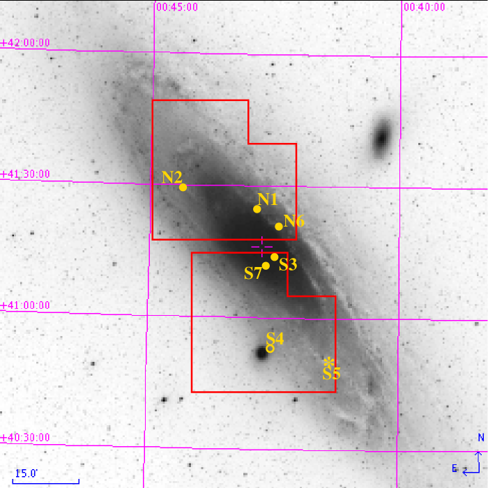
Figure 1: Projected on M31, we display the boundaries of the observed fields (red lines), and the centre of M31 (cross). Circles mark the positions of the 6 microlensing events issued from the selection pipeline (Sect. 3.1). The open circle (S4) corresponds to the event seen toward M32. The star (S5) to the binary event candidate discussed in Sect. 3.3.

2.2 Analysis: selection of microlensing events

To search for microlensing events, we use the “pixel-lensing” technique (Baillon et al. 1993; Gould 1996; Ansari et al. 1997), in which one monitors the flux variations of unresolved sources of each pixel element of the image.

A difficulty, specific to pixel lensing, is that genuine microlensing events might be polluted by one of the numerous variable objects present in the neighbouring pixels. To avoid loosing too many bona fide microlensing events while accounting for the variable background, we look for microlensing-like variations even on those light curves on which a second bump is detected. In particular, on each light curve we first look for and characterise mono-bump variations for each season separately. Only as a final step do we test for bump uniqueness on the complete light curve in a loose way as explained below. This test allows for the presence of variable stars within the superpixel containing the lensed source and so, as a bonus, in principle could allow us to detect microlensing of variable objects.

In addition to the physical background of variable stars, the search for microlensing-like flux variations, in particular the short ones, is plagued by the detection of “fake” variations, mainly due to bad images, defects on the CCD, saturated pixels associated with extremely bright stars, and cosmic rays (these issues are discussed in more detail in Tsapras et al. 2005). The only safe way to remove these artefacts is to visually inspect the images around the time of maximum, although there may be other useful hints, such as an anomalous distribution of the times of maximum or in the spatial distribution. To obtain a “clean” set of variations we first run the complete pipeline, identify and remove bad images, and mask bad pixels. Then, we rerun the analysis from scratch.

Before proceeding further with the pipeline, we mask a small region right around the centre of M31, $\sim 1^{\prime}\times 1^{\prime}$, where, in addition to problems caused by saturation, the severe uncertainty in modelling the experiment would prevent us from drawing any significant conclusion about the physical implication of any result we might obtain.

As a first step, we establish a catalogue of significant flux variations (using the $r$ band data only, which are both better sampled and less seriously contaminated by intrinsically variable stars than the $i$ band data). Following Calchi Novati et al. (2003), we use the two estimators, $L$ and $Q$, which are both monotonic functions of the significance of a flux variation, to select candidates. Note that the previous POINT-AGAPE selections presented in Paulin-Henriksson et al. (2003); An et al. (2004a); Belokurov et al. (2005), have been carried out using the $L$ estimator only.

We define

$$L=-\ln\left(\Pi_{j\in bump}P(\Phi|\Phi>\Phi_{j})\right)\;\;\mbox{given}\;\;\bar{\Phi}_{bkg},\,\sigma_{j}\,,$$ (1)

where

$$P(\Phi|\Phi>\Phi_{j})=\int_{\Phi_{j}}^{\infty}d\Phi{\frac{1}{\sigma_{j}\sqrt{2\pi}}}\exp\left[{-\frac{(\Phi-\bar{\Phi}_{bkg})^{2}}{2\sigma_{j}^{2}}}\right];$$ (2)

$\Phi_{j}$ and $\sigma_{j}$ are the flux and associated error in a superpixel at time $t_{j}$, $\bar{\Phi}_{bkg}$ is an estimator of the baseline level, defined as the minimum value of a sliding average over 18 epochs. A “bump” is defined as a positive variation with at least 3 consecutive points more than $3\,\sigma$ above the baseline, and it is regarded as ending after two consecutive points less than this threshold. We define

$$Q\equiv\frac{\chi^{2}_{const}-\chi^{2}_{pacz}}{\chi^{2}_{pacz}/\rm dof}\,,$$ (3)

where $\chi^{2}_{const}$ is calculated with respect to the constant-flux hypothesis and $\chi^{2}_{pacz}$ is the $\chi^{2}$ calculated with respect to a Paczyński fit. Let us stress that $Q$ is evaluated for each full season, while $L$ is evaluated only inside the bump. At this point, we keep only light curves with $Q>100$. Since $Q$ is biased toward mono-bump variations, this step allows us to remove the unwanted background of short-period variable stars.

Although it has already been described in Calchi Novati et al. 2002 , we return to a crucial step of the above analysis. For each physical variation, there appears a whole cluster of pixels with $Q>100$ (with typical size range from 4 to 30 pixels). From the $Q$ values of all light curves, we construct a $Q$ map for each season. We then proceed to the actual localisation of the physical variations. First we identify the clusters (which appear as hills on the map). Then we locate the centre of the cluster as the pixel with the highest value of the $L$ estimator. The main difficulty arises from the overlap of clusters. Indeed we must balance the search for faint variations with the need to separate neighbouring clusters. In the following, we will refer to this crucial part of the analysis as “cluster detection”. It must be emphasised that this step cannot be carried out on separate light curves, but requires using $Q$ maps. The impossibility of including this cluster detection in the Monte Carlo  (Sect. 4) gives us one of the strongest motivations for the detection efficiency analysis described in Sect. 5. After the clusterisation, we are left with $\sim 10^{5}$ variations.

The following part of the analysis is carried out working only on pixel light curves.

As a second cut, we remove flux variations having too small a signal-to-noise ratio (most likely due to noise) by demanding $L_{1}>40$, $L_{1}$ being associated with the bump. If the light curve shows a second bump over the three seasons, characterised by $L_{2}$, we then demand that this satisfies $L_{2}<0.5L_{1}$. As we are only looking for bright bumps (see below), we consider such a significant second bump to indicate that these bumps most likely belong to a variable star.

We estimate the probability for the lightcurve of a given event to be contaminated by a nearby variable source as the fraction of pixels showing a significant variation, $L_{1}>40$. This fraction stronlgy depends on the distance from the centre of M31: from $\sim 10\%-20\%$ in the inner M31 region, within an angular radius of $8^{\prime}$, down to $\sim 8\%$ in the outer region.

We characterise the shape of the variation by studying its compatibility with a Paczyński (1986) shape. We perform a two-band 7-parameter fit: the Einstein time, $t_{\textrm{E}}$, the impact parameter, $u_{0}$, the time at maximum magnification $t_{0}$, and the band dependent flux of the unresolved source, $\phi^{*}$, and the background flux, $\phi_{b}$, of the bump in each of 2 bands ($r$ and either $i$ or $g$ according to the available data along the bump). Throughout the analysis we use, as an observable time width, the full-width-half-maximum (FWHM) in time of the Paczyński curve, $t_{1/2}$, and the flux increase $\Delta\Phi$ of the bump, both of which are functions of the degenerate parameters $t_{\textrm{E}},\,u_{0}$ and $\phi^{*}$ (Gould 1996). Using the flux deviation in the two bands, we evaluate in the standard Johnson/Cousins magnitude system $R(\Delta\Phi)$, the “magnitude at maximum” of the bump, and its colour, either $V-R$ or $R-I$. The simultaneous Paczyński fit in two bands effectively provides a test of the achromaticity expected for microlensing events.

As a third cut, we use the goodness of the Paczyński fit as measured by the reduced $\chi^{2}$. For short events, the behaviour of the baseline would dominate the $\chi^{2}$. To avoid this bias, we perform the fit in a smaller “bump region” defined as follows. A first Paczyński fit on the whole baseline provides us with the value of the baseline flux $\phi_{b}$ and first estimates of the time of maximum magnification $t_{0}$ and the time width $t_{1/2}$. Using these values we compare two possible definitions of the bump region and use whichever is the larger of: (i) the time interval inside $t_{0}\pm 3\,t_{1/2}$, and (ii) the time interval that begins and ends with the first two consecutive points less than 3 $\sigma$ above the background on both sides of $t_{0}$. The final Paczyński fit is carried out in this “bump region” with the basis flux $\phi_{b}$ fixed in both colours, and this fit provides the values of the 5 remaining parameters.

Our third selection criterion excludes light curves with $\chi^{2}/\textrm{dof}>10$.

We fix this threshold high enough to accept light curves whose shapes slightly deviate from the Paczyński form, either because of a real deviation in the microlensing signal, as is the case for the microlensing event PA-99-N2 discussed by An et al. (2004b), or because the signal may be disturbed by artefacts or by some nearby variable stars.

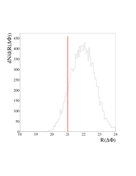
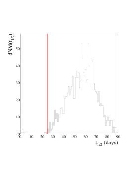
Figure 2: Top: Distribution of flux deviations at maximum for the selected events after the sampling cut. Bottom: Duration distribution for the selected events after the cut on $R(\Delta\Phi)$.

Figure 3: $r$ and $i$ filter 3-year light curves for 2 selected variations before the last cut. Upper panels, PA-99-N1, an accepted candidate. Lower panels: a rejected candidate. The dashed line is the best-fit for a Paczyński bump with a sinusoidal background. The abscissae are time in days (JD-2451392.5). The ordinates are flux in ADU/s.

criterion	number of selected light curves
cluster detection ($Q>100$)	$\sim 10^{5}$
signal to noise ratio ($L_{1}>40$) and second bump ($L_{2}/L_{1}<0.5$)	$\sim 4\cdot 10^{4}$
shape analysis : $\chi^{2}/\textrm{dof}<10$ (7 parameter Paczyński fit)	$\sim 3\cdot 10^{4}$
time sampling along the bump	$\sim 10^{4}$
flux deviation: $R(\Delta\Phi)<21$	$\sim 1.5\cdot 10^{3}$
time width: $t_{1/2}<25$ days	9
second bump analysis	6

Table 1: Summary of the selection criteria and number of the selected light curves.

	PA-99-N1	PA-99-N2	PA-00-S3	PA-00-S4
$\alpha$ (J2000)	00h42m51.19s	00h44m20.92s	00h42m30.27s	00h42m29.98s
$\delta$ (J2000)	$41^{\circ}23^{\prime}56.3^{\prime\prime}$	$41^{\circ}28^{\prime}44.8^{\prime\prime}$	$41^{\circ}13^{\prime}00.6^{\prime\prime}$	$40^{\circ}53^{\prime}46.1^{\prime\prime}$
$\Delta\Theta$	$7^{\prime}53^{\prime\prime}$	$22^{\prime}04^{\prime\prime}$	$4^{\prime}06^{\prime\prime}$	$22^{\prime}33^{\prime\prime}$
$t_{1/2}$ (days)	$1.83^{+0.12}_{-0.11}$	$22.16^{+0.12}_{-0.12}$	$2.303^{+0.074}_{-0.062}$	$1.96^{+0.09}_{-0.10}$
$R(\Delta\Phi)$	$20.83\pm 0.10$	$19.10\pm 0.10$	$18.80\pm 0.20$	$20.7\pm 0.20$
$V-R$	$1.2\pm 0.2$	$1.0\pm 0.1$
$R-I$			$0.6\pm 0.1$	$0.0\pm 0.1$
$t_{0}$ (JD-2451392.5)	$13.85\pm 0.05$	$71.70\pm 0.10$	$458.40\pm 0.02$	$488.90\pm 0.07$
$t_{\rm E}$ (days)	$8.3^{+4.5}_{-2.7}$	$71.1^{+4.1}_{-3.7}$	$10.4^{+2.5}_{-2.3}$	$135^{+??}_{-76}$
$u_{0}$	$0.070^{+0.046}_{-0.030}$	$0.1014^{+0.0070}_{-0.0067}$	$0.070^{+0.024}_{-0.017}$	$0.0042^{+0.056}_{-??}$
$\phi_{r}^{*}$ (ADU/s)	$1.17^{+0.76}_{-0.49}$	$10.87^{+0.77}_{-0.83}$	$8.9^{+3.3}_{-2.1}$	$0.11^{+0.15}_{-??}$
$\phi_{g}^{*}$ (ADU/s)	$0.35^{+0.24}_{-0.15}$	$3.57^{+0.28}_{-0.25}$
$\phi_{i}^{*}$ (ADU/s)			$11.7^{+4.0}_{-2.9}$	$0.07^{+0.10}_{-??}$
$A_{\textrm{max}}$	$14.3^{+9.4}_{-6.1}$	$9.9^{+0.68}_{-0.65}$	$14.3^{+4.9}_{-3.5}$	$200^{+3200}_{-??}$
$\chi^{2}/$dof	1.1	9.3	2.1	0.9

Table 2: Main characteristics of the four already published microlensing candidates. $\Delta\Theta$ is the projected separation from the centre of M31. The magnitudes correspond to the maximum flux deviation and are given in standard Johnson/Cousins system. The results reported here are the results of the Paczyński fit alone, even when extra information is available, as is the case for PA-99-N1 and PA-99-N2.

Another crucial element in the selection is the choice for the required sampling along the bump. In fact, while a good sampling is needed in order to meaningfully characterise the detected variation, demanding too much in this respect could lead us to exclude many bona fide candidates. Using the values of $t_{1/2}$ and $t_{0}$ determined in the preceding step, we define 4 time intervals around the time of maximum magnification $t_{0}$: $[t_{0}-3\,t_{1/2},\,t_{0}-t_{1/2}/2],\,[t_{0}-t_{1/2}/2,\,t_{0}],\,[t_{0},\,t_{0}+t_{1/2}/2]$ and $[t_{0}+t_{1/2}/2,\,t_{0}+3\,t_{1/2}]$. As a fourth cut we demand that a minimum number of observing epochs $n_{min}$ occur in each of at least 3 of these time intervals. Clearly $n_{min}$ cannot be as large for short events as for long ones. We choose $n_{min}=1,\,2$ and 3 for $t_{1/2}<5,\,t_{1/2}\in(5,15)$ and $t_{1/2}>15$ days, respectively. Furthermore, neither of the external intervals should fall at the beginning or end of one of the three seasons and at the same time be empty.

The cuts described above reduce our sample of potential events to $\sim 10^{4}$, about one tenth of the initial set of selected variations, but still mostly variable stars.

In this paper, we restrict attention to bright microlensing-like variations, in particular we demand $R(\Delta\Phi)<21$, although the observed deviations extend down to $R(\Delta\Phi)\sim 24$ (Fig. 3). This reduces our set of candidates by another factor of $\sim$ 10.

The Monte Carlo (Sect. 4) predicts most of the microlensing events to be rather short. On the other hand, the observed $t_{1/2}$ distribution shows a clustering of long variations centred on $t_{1/2}\sim 60$ days, most of which are likely to be intrinsically variable objects, and a much smaller set of short-duration variations (Fig. 3). We demand $t_{1/2}<25$ days, which leaves us with only 9 Paczyński-like flux variations.

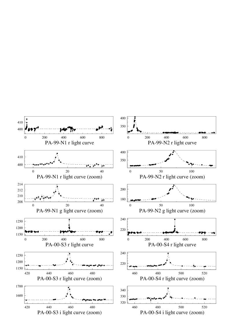
Figure 4: 3-year light curves of the four microlensing events PA-99-N1, PA-99-N2, PA-00-S3 and PA-00-S4. For each event, the top panel shows the whole light curve in the $r$ filter, while the 2 lower panels display zoomed light curves in all bands for which data are available. Dashed lines are best-fit Paczyński curves. The abscissae are time in days (JD-2451392.5). The ordinates are flux in ADU/s.

Out of the 9 variations selected above, 5 show a significant second bump. We want to exclude variable stars, while keeping real microlensing variations that happen to be superimposed on a variable signal. For most variable stars the secondary bump should be rather similar but not identical to the detected one. To make use of this fact we perform a three-colour fit, modelling the light curve with a Paczyński bump plus a sinusoidal signal, and then compare the time width and the flux variation of the sinusoidal part with those of the Paczyński bump. Because our model is very crude and because we know that variable stars may show an irregular time behaviour, we do not ask for a strict repetition of the bump along the baseline to reject a variation. We exclude a light curve if both the $R(\Delta\Phi)$ difference between the two bumps is smaller than 1 magnitude and the time width of the sinusoidal part is compatible with that of the bump within a factor of 2. Three out of nine variations are excluded in this step. For all three the detected bump is relatively long ($t_{1/2}>$ 20 days) and faint ($R(\Delta\Phi)>20.5$). Furthermore, on the images the position of the second bump appears to be consistent with that of the detected bump, clear evidence in favour of the intrinsically variable origin of these variations. Two other light curves are retained, although they show a significant secondary bump; in both cases, the secondary bump is much longer than the main one. Besides, in both cases the direct inspection on the images reveals that the position of the second bump is different from that of the detected one. In order to make clear the sense of the present criterion, we show (Fig. 3) the result of the Paczyński fit superimposed over a sinusoidal background for two variations. In the upper panels is an accepted candidate, for which the short and bright bump at $t_{0}\sim 13$ (JD-2451392.5) is clearly distinct from the underlying variable signal. In the lower panels is a rejected candidate. The Paczyński signal originally selected with peak at $t_{0}\sim 480$ (JD-2451392.5) is clearly undistinguishable from the underlying variable background.

We are now left with our final selection of 6 light curves showing an achromatic, short-duration and bright flux variation compatible with a Paczyński shape. We denote them PA-99-N1, PA-99-N2, PA-00-S3, PA-00-S4, PA-00-N6 and PA-99-S7. The letter N(S) indicates whether the event lies in the north (south) INT WFC field, the first number (99, 00, or 01) gives the year during which the maximum occurs, and the second has been assigned sequentially, according to when the event was identified.

In Table 2 we report in sequence each step of the pipeline with the number of the selected candidates remaining.

3 Microlensing events

3.1 POINT-AGAPE 3 years analysis results

In this section we look at the 6 selected candidates in detail. In Table 2 and Figure 4 we recall the characteristics and light curves of the four already published candidates, while Table 3 and Figures 6 and 6 are devoted to the two new ones. The errors in $R(\Delta\Phi)$ and the colour index are dominated by the uncertainty in the calibration of the observed flux with respect to the standard magnitude system, except for PA-00-N6. When the 7-parameter Paczyński fit does not converge properly, the time width and the flux increase are estimated from a degenerate fit (Gould 1996).

Figure 5: 3-year light curves of the microlensing event PA-00-N6. Panels and symbols as in Figure 4.

Figure 6: 3-year light curves of the microlensing event PA-99-S7. Panels and symbols as in Figure 4.

	PA-00-N6	PA-99-S7
$\alpha$ (J2000)	00h42m10.70s	00h42m42.56s
$\delta$ (J2000)	$41^{\circ}19^{\prime}45.4^{\prime\prime}$	$41^{\circ}12^{\prime}42.8^{\prime\prime}$
$\Delta\Theta$	$7^{\prime}16^{\prime\prime}$	$3^{\prime}28^{\prime\prime}$
$t_{1/2}$ (days)	$1.77^{+0.57}_{-0.60}$	$4.10^{+0.85}_{-0.73}$
$R(\Delta\Phi)$	$20.78^{+0.18}_{-0.31}$	$20.80\pm 0.10$
$V-R$		$0.79\pm 0.14$
$R-I$	$0.51^{+0.25}_{-0.43}$
$t_{0}$	$491.30\pm 0.07$	$65.21\pm 0.14$
$t_{\rm E}$ (days)	$8.3^{+10.5}_{-4.1}$	-
$u_{0}$	$0.07^{+0.13}_{-0.052}$	-
$\phi_{r}^{*}$ (ADU/s)	$1.40^{+2.6}_{-0.95}$	-
$\phi_{i}^{*}$ (ADU/s)	$1.7^{+3.2}_{-1.2}$	-
$A_{\textrm{max}}$	$14^{+26}_{-11}$	-
$\chi^{2}/$dof	1.0	1.3

Table 3: Main characteristics of the two new microlensing candidates. The parameters are the same as in Table 2.

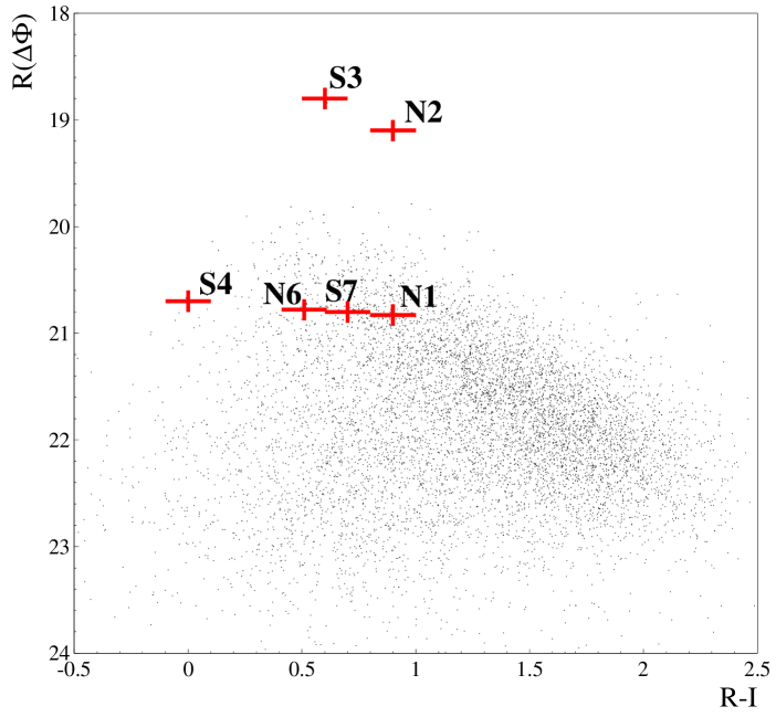
Figure 7: $R(\Delta\Phi)-(R-I)$ colour-magnitude diagram for the $\sim 10\,000$ variations selected before the cut on the flux deviation at maximum. Superimposed we show the positions of the 6 selected candidates. The $R-I$ colours for $PA-99-N2$ and $PA-99-S7$ are estimates derived from the observed $V-R$ colours.

The source star of PA-99-N1 has been identified on HST archival images (Aurière et al. 2001). Fixing the source flux at the observed values, $\phi^{*}_{r}=1.02\,\mathrm{ADU/s}$ and $\phi^{*}_{g}=0.28\,\mathrm{ADU/s}$, we obtain $t_{\textrm{E}}=9.20\pm 0.61$ days and $u_{0}=0.060\pm 0.005$, compatible within $1\sigma$ with the values reported in Table 2, obtained from our data alone. Finally, the HST data allow us to estimate the colour $(R-I)\sim 0.9$. In An et al. (2004b), we have demonstrated that PA-99-N2, which shows significant deviations from a simple Paczyński form, is compatible with microlensing by a binary lens. The binary-fit parameters are characterised by a longer time scale and higher magnification than the point-lens fit. In the best-fit solution we find $t_{\textrm{E}}=125.0\pm 7.2$ days, $u_{0}=(3.60\pm 0.37)\times 10^{-2}$, $\phi^{*}_{r}=4.76\pm 0.34$ ADU/s, and a lens mass ratio $\sim 1.2\times 10^{-2}$. Under the assumption that the lens is associated with M31 (rather than the MW), the lower bounds on the angular Einstein radius ($\theta_{\rm E}>25\,\mu\rm as$) deduced from the absence of detectable finite-source effects implies that the source-lens relative velocity is $v_{\perp}>280$ km/s, and the source-lens distance is $d_{ls}>45\,{\mathrm{kpc}}(M/M_{\odot})^{-1}$, where $M$ is the lens mass. These facts, together with PA-99-N2’s large distance from the M31 centre ($\sim 22^{\prime}$) make it very unlikely to be due to an M31 star, while the prior probability that it is due to a MW star is extremely low. Hence, PA-99-N2 is a very strong MACHO candidate (either in M31 or the MW). The sampling and the data quality along the bump are also good enough to permit a reliable estimate of all 7 parameters of the Paczyński fit for the event PA-00-S3. For PA-00-S4 we obtain only a reliable lower limit on $t_{\textrm{E}}$, and accordingly an upper limit on $u_{0}$, as indicated by the question marks in Table 2.

For PA-00-N6, the data allow us to evaluate the full set of Paczyński parameters. Note the rather short Einstein time, $\sim 10$ days, similar to those of PA-99-N1 and PA-00-S3.

As in the case of PA-99-N1 (Paulin-Henriksson et al. 2003), PA-99-S7 lies near (within 4 pixels) of a long-period red variable star. This induces a secondary bump, which is particularly visible in the $i$ light curve. PA-99-S7 has been accepted by the last step of our selection pipeline, despite this second bump being responsible for poor stability of the baseline. In this case, the data do not allow us to break the degeneracy among the Paczyński parameters and therefore do not allow a reliable estimate of the Einstein time.

A colour-magnitude diagram of the $\sim 10\,000$ variations selected after the sampling cut is shown in Figure 7. Superimposed we indicate the position of the 6 variations finally selected after all cuts. In particular, we note the peculiar position of PA-99-N2, which (together with PA-00-S3) is unusually bright relative to the other variations. Recall that PA-99-N2 is also the longest selected variation, with $t_{1/2}\sim 22$ days. As we have already excluded short-period variables, the sample shown is dominated by red, long-period variables of the Mira type with $R(\Delta\Phi)>21,\,(R-I)>1$. For a detailed discussion of the variable star populations detected within our dataset see An et al. (2004a).

The spatial position for the detected events projected on the sky is shown, together with the INT fields, in Figure 1. Note the two new events are located within a rather small projected distance of M31’s centre.

3.2 Variable Contamination

Probably the biggest single problem in the interpretation of microlensing events drawn from faint sources is the possibility that the sample may be contaminated with rare variables. For relatively bright sources, such as those being detected by the thousand toward the Galactic bulge (Udalski 2003), microlensing events are easily distinguished from variables by their distinct shape. However, as the S/N declines, such discrimination becomes more difficult. Experiments toward the LMC provide sobering confirmation of the legitimacy of this concern. Both of the original microlensing candidates reported by the EROS collaboration (Aubourg et al. 1993) were subsequently found to be variable stars, while some candidates found by the MACHO collaboration (Alcock et al. 1997, 2000) were also subsequently recognized as possible or certain variables. The SuperMACHO collaboration (Becker et al. 2004), which probes about 2 mags fainter than MACHO or EROS in its microlensing search toward the LMC, has so far found it extremely difficult to distinguish between genuine microlensing events and background supernovae (C. Stubbs 2005, private communication). Thus, when reporting a handful of microlensing candidates drawn from 3 years of monitoring of a large fraction of an entire L* galaxy, we should cautiously assess the possibility of variable contamination.

If variables were contaminating our sample, they would have to reside either in the MW or in M31 itself, or they could be background supernovae. We consider these locations in turn.

There are three arguments against MW variables: distribution on the sky, absence of such variables in the Galactic microlensing studies, and lack of known classes of Galactic variables that could mimic microlensing. First, of the 5 microlensing candidates that enter our event-rate analysis (i.e., excluding the intergalactic microlensing candidate PA-00-S4), 4 lie projected in or near the M31 bulge. This strongly argues that they are, in their majority, due to M31 sources, which are also heavily concentrated in this region. By contrast, Galactic variables would be spread uniformly over the entire field. Of course, this does not rule out the possibility of minor contamination by such variables.

However, if there were a class of variables that could even weakly mimic short microlensing events with flux variations corresponding to $R(\Delta\Phi)<21$, then these would have easily shown up in Galactic microlensing experiments. For example, the OGLE-III microlensing survey covers over 50 deg² toward the Galactic bulge, more than 100 times larger than our survey toward M31. The OGLE survey does not go as deep as ours because their telescope is smaller (1.3m) and their exposure times are shorter (2 min), although these factors are somewhat compensated by their denser temporal coverage. Ignoring this shallower depth for the moment, and restricting consideration to $\la 3\,\rm kpc$ (where most of our foreground MW disc stars lie) the projected density of disc stars is about 10 times higher in the OGLE fields than in ours because they lie at lower Galactic latitude. Hence, one would expect of order 1000 times more such variables to appear in the OGLE fields than in ours. Of course, the majority of these would be $R(\Delta\Phi)\sim 21$ and so of such low signal-to-noise ratio that they would not appear as OGLE candidates, or if they did, would escape recognition as variables. However, $\sim 1/125$ would lie 5 times closer and so be 3.5 mag brighter, i.e., $R(\Delta\Phi)<17.5$, corresponding to $I\la 17$, and these would have good signal-to-noise ratio. No such variable population is reported. A similar argument applies to Galactic halo stars, which would also be much denser in the OGLE-III fields than in ours.

Third, there are no known candidate classes of Galactic variables that could mimic the M31 microlensing events. The one possibility is dwarf-novae, which have been reported as faking microlensing events toward the LMC (Ansari et al. 1995) and M22 (Bond et al. 2005). However, with typical peak absolute magnitudes of $M_{V}\sim 2$ (Warner 1995), they would have to lie well outside the Galaxy to appear as $R(\Delta\Phi)\sim 21$ fluctuations.

While the case against M31 variables is not as airtight as against Galactic ones, it is still quite strong. The basic argument is that if the sources are in M31, then they must suffer luminosity changes corresponding to $M_{R}<-3.5$ on quite short timescales ($t_{1/2}<5\,$days for all candidates except PA-99-N2). There are no known classes of variables that do this except for novae. However, novae show brighter variations and strongly asymmetric light curves characterized by slow descents (a selection of novae variations in our dataset is discussed in Darnley et al. 2004). While in principle our microlensing candidates could be due to some new, so far unrecognized (nor even conjectured) type of stellar variability, the great brightness and very short timescale of the observed events impose severe restrictions on candidate mechanisms of variability.

Novel mechanisms to explain the sixth event, PA-99-N2, would be less constrained because it is much longer, $t_{1/2}\sim 22\,$days. However, being long as well as very bright ($R(\Delta\Phi)\sim 19$), its signal-to-noise ratio is quite high. This permits us to check for achromaticity with very good precision. Even the deviations from a simple Paczyński shape are achromatic and can be reproduced by a binary-lensing curve (An et al. 2004b). That is, PA-99-N2 is an excellent microlensing candidate on internal evidence alone.

Finally, we remark on supernovae which, as noted above, plague the SuperMACHO project and also were a difficult contaminant for the MACHO and EROS projects. There are two principal arguments against supernovae. First, the FWHMs of all but one of the events are too short for supernovae while, as we have just argued, the sixth event is achromatic and fit by a binary-lens light curve and therefore almost certainly microlensing. Second supernovae cannot be responsible for the majority of the events because the supernovae would be uniformly distributed on the sky while the actual events are highly clustered near the centre of M31.

For completeness, we address one other concern related to variability: the possibility that the source displays a signature of variability away from the microlensing event. In this case, one might worry that this “event” is actually an outburst from an otherwise low-level variable. Recall that our selection procedure actually allows for a superpixel to show lower-level variability in addition to the primary “event” that is characterized as microlensing, and to still be selected as a candidate. This is necessary because about 15% of pixel light curves within $8^{\prime}$ of the M31 centre (a region containing most of our events) show variable-induced “bumps” with likelihood $L_{1}>40$. So we would lose 15% of our sensitivity if we did not try to recover microlensing events with such secondary bumps. One event (PA-99-N1) out of four in this region displays such a severe secondary bump. This 25% rate is within Poisson uncertainties of the 15% expectation. In addition, a second event (PA-99-S7) displays a secondary bump at less than half this threshold.

It must be stressed, however, that through a Lomb analysis we find that neither of the source stars for these two events shows any sign of variability apart from the microlensing event. In both cases, the source of the lower-level variation lies several pixels from the microlensing event.

In brief, while we cannot absolutely rule out non-microlensing sources of stellar variability, all scenarios that would invoke variability to explain our candidate list are extremely constrained, indeed contrived.

3.3 A likely binary event

Our selection pipeline is deliberately biased to reject flux variations that strongly differ from a standard Paczyński light curve. In particular, it cannot detect binary lens events with caustic crossing. We discuss here a blue flux variation ($R-I\sim 0$) that failed to pass the $\chi^{2}$ cut, but is most probably a binary lens event: PA-00-S5. The light curve, which involves a short ($t_{1/2}\sim 2\mbox{ days}$) and bright peak followed by a plateau, is suggestive of binary lensing with a caustic crossing. The photometric follow-up of this event is tricky, particularly in the $i$ band, because a faint resolved red object lies about 1.5 pixels away. To overcome this difficulty, we have used a more refined difference image photometry that includes modelling the PSF.

We have found a binary lensing solution that convincingly reproduces the shape of the bump. The corresponding light curve, superimposed on the data obtained using difference image photometry, is displayed in Figure 8, where we show the full $r$ light curve, zooms of the bump region in the $r$ and $i$ bands, and the ratio of flux increases $\Delta\Phi_{r}/\Delta\Phi_{i}$.

Figure 8: A binary solution superposed on the differential-photometry light curve of the binary-lens candidate PA-00-S5. Upper panel: full $r$ light curve; middle panels: $r$ and $i$ zooms around the bump region, the dotted line shows the baseline; bottom panel: the colour ratio $\Delta\Phi_{r}/\Delta\Phi_{i}$, the dash-dotted line being the average colour ratio. The abscissae are time in days (JD-2451392.5), the ordinates of the three upper panels are flux in ADU/s.

This solution is a guess, neither optimised nor checked for uniqueness. The parameters are as follows: the distance between the two masses is $d=0.63$ in unit of the Einstein radius $R_{E}$, the mass ratio is $q=1/2$; the distance of closest approach to the barycentre, $u_{0}=0.17$, is reached at $t_{0}=411\mbox{(JD-2451392.5)}$; the Einstein time scale is $t_{E}=50\mbox{ days}$; the source crosses the binary axis at an angle of $58.5^{\circ}$, outside the two lenses and close to the heavy one.

The location of PA-00-S5 is $\alpha$ = 00h41m14.54s, $\delta=40^{\circ}48^{\prime}37.7^{\prime\prime}$, J2000, some $32^{\prime}$ away from M31’s centre. This event cannot enter the discussion of the following sections because it does not survive our full selection pipeline and because the possibility of caustic crossings is not included in the simulation. Nevertheless, if this event is due to microlensing, the lens is most probably a binary MACHO.

3.4 Comparison with other surveys

The first microlensing candidate reported in the direction of M31, AGAPE-Z1, was detected in 1995 by the AGAPE collaboration (Ansari et al. 1999). AGAPE-Z1 is a very bright event, $R=17.9$, of short duration, $t_{1/2}$ =5.3 days, and located in the very central region of M31, at only $\sim 42^{\prime\prime}$ from the centre.

The MEGA collaboration has presented results from a search for microlensing events using the first 2 years of the same 3-year data set analyzed here (de Jong et al. 2004), but a different technique. In contrast to the present analysis, they do not impose any restriction on $t_{1/2}$ and $R(\Delta\Phi)$. As a result, they select 14 microlensing candidates. All of them belong to our initial catalogue of flux variations. However, beside MEGA-7 and MEGA-11 (corresponding to PA-99-N2 and PA-00-S4, respectively), the remaining 12 flux variations are fainter than allowed by our magnitude cut ($R(\Delta\Phi)<21$). Moreover, MEGA-4, MEGA-10, MEGA-12 and MEGA-13 have time widths longer than our threshold of 25 days.

The WeCAPP collaboration, using an original set of data acquired in the same period as our campaign, reported the detection of two microlensing candidates (Riffeser et al. 2003). The candidate WeCAPP-GL1 is PA-00-S3. We did not detect the candidate WeCAPP-GL2 (short enough but probably too faint to be included in our selection) because its peak falls in a gap in our observations.

The NAINITAL survey has recently reported (Joshi et al. 2005) the discovery of a microlensing candidate toward M31, quite bright ($R(\Delta\Phi)=20.1$) but too long ($t_{1/2}\sim 60$ days) to be selected within our pipeline.

Recently we have reported (Belokurov et al. 2005) the results of a search for microlensing events obtained using a different approach. Starting from a different catalogue of flux variations and using a different set of selection criteria (in particular, we did not include any explicit cut in $t_{1/2}$ or $R(\Delta\Phi)$), we reported 3 microlensing candidates: PA-00-S3, PA-00-S4 and a third one, which is not included in the present selection. It is a short, bright, rather blue flux variation ($t_{1/2}=4.1$ days, $R(\Delta\Phi)=19.7$, $R-I=0.0$), detected in the third year ($t_{0}=771$ (JD-2451392.5)). In the present analysis it is rejected because it fails to pass the sampling cut: it does not have enough points on the rising side to safely constrain its shape. The position of this event, ($\alpha$=00h42m02.35s, $\delta=40^{\circ}54^{\prime}34.9^{\prime\prime}$, J2000), rather far away from the centre of M31 ($\Delta\Theta=22^{\prime}59^{\prime\prime}$), is consistent with its being a MACHO candidate. However, because it does not survive the present selection pipeline, we do not include it in the following discussion. A further analysis in which we follow a still different approach is currently underway (Tsapras et al. 2005).

4 The Monte Carlo analysis

The Monte Carlo attempts, for a given astrophysical context, to predict the number of events expected in our experiment, trying to mimic the observational conditions and the selection process. Because these can only partially be included in the Monte Carlo, the full simulation of our observation campaign must involve the detection efficiency analysis which is described in Sect. 5.

4.1 The astrophysical model

4.1.1 The source stars

Source stars are drawn according to the target M31 luminosity profile as modelled by Kent (1989). The 3-dimensional distribution of bulge stars is also taken from Kent (1989). The distance $z$ of disc stars to the disc plane follow a $1/\cosh^{2}(z/H)$ distribution with $H=0.3\,{\mathrm{kpc}}$ as proposed by Kerins et al. (2001).

The colour-magnitude distributions of disc and bulge stars are supposed to have the characteristics of the Milky Way disc and bulge populations. The distribution of disc stars is taken from the solar neighbourhood data obtained by Hipparcos (Perryman et al. 1997), corrected at the bright end for the completeness volume and incorporating at low luminosity (needed for normalisation) a Besançon disc model (Robin et al. 2003). For the bulge we again use a Besançon model (Robin et al. 2003) completed at the faint end using Han & Gould (1996). We construct two distinct types of “colour-magnitude diagrams” (CMDs) from the Monte Carlo and show these in Figure 9 with the position of the actual detected events superposed. The first is a standard CMD, which plots apparent magnitude versus colour for the sources of all the simulated microlensing events that meet our selection criteria. In fact, however, while the colours and magnitudes of all selected-event sources are “known” in the Monte Carlo, they cannot always be reliably extracted from the actual light curves: the colours are well-determined, but the source magnitudes can only be derived from a well-constrained Paczyński fit (while some events have only degenerate fits). We therefore also show in Figure 9 a second type of CMD, in which the ordinate is the magnitude corresponding to maximum flux increase during the event ($R(\Delta\Phi)$). It is always well-determined in both the Monte Carlo and the data.

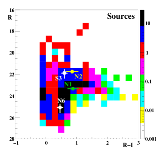
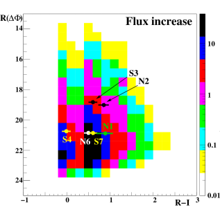
Figure 9: The colour/magnitude event density distribution predicted by the Monte Carlo. Top panel: R magnitude of the source star. Bottom panel: R magnitude of the flux increase. The observed events are superposed on the diagrams. Only those events for which the source magnitude can be reliably extracted appear in the left panel. The colour scale shows the event density (in arbitrary units).

To take into account the effect of the finite size of stars, which can be important for low mass MACHOs, we have to evaluate the source radii. To this end, we use a colour temperature relation evaluated from the models of Robin et al. (2003), and we evaluate the radii from Stefan’s law using a table of bolometric corrections from Murdin (2001).

We did not take into account possible variations of the interstellar extinction across the field, although there are indications of higher extinction on the near side (An et al. 2004a). The best indicator we have of differential extinction is the asymmetry of the surface brightness map, and this gives a flux attenuation by dust on the near side of about 10%. This is also the order of magnitude of the average extinction one would obtain assuming that the M31 disc absorption is about twice that of the MW disc. Indeed, as dust is confined in a thin layer, extinction only significantly affects the stars on the back side. Clearly an attenuation of about 10% would not significantly affect the results presented here.

4.1.2 The lenses

The lenses can be stars or halo objects, with the latter being referred to as “MACHOs”. The stellar lenses can be either M31 bulge or disc stars.

In the case of the bulge, we shall consider the microlensing contribution of bulge stars with a standard stellar mass-to-light ratio. Such models form the only true litmus test for whether or not dark matter must be invoked, since the dark matter solution is classically required to explain observations which cannot be accounted for by known populations. The only dynamical requirement for our stellar bulge models is that their dynamical contribution does not exceed the observed inner rotation curve. They do not need to fully reproduce the inner rotation curve, though their failure to do so must be seen as evidence in itself for dark matter. We shall from here onwards use the term stellar bulge to denote the contribution to the bulge from ordinary stars. We use the term bulge by itself to mean the entire dynamical bulge mass, which must include the stellar bulge but which may also comprise additional mass from unknown populations. We implicitly assume that the total bulge mass is fixed by the rotation curve. We set out here to discover whether or not the rate predicted by known stellar bulge and disc populations can feasibly account for our observed microlensing candidates.

Disk stellar lenses

The disc mass distribution is the same as in Kerins et al. (2001):

$$\rho=\rho_{0}\exp\left(-\frac{r}{h}\right)/\cosh^{2}\left(\frac{z}{H}\right)$$

with $\rho_{0}=0.3\,M_{\odot}\,{\mathrm{pc}}^{-3}$, $H=0.3\,{\mathrm{kpc}}$ and $h=6.4\,{\mathrm{kpc}}$.

The mass of the disc is $3\,10^{10}\,M_{\odot}$, corresponding to an average disc mass-to-light ratio ${M/L}_{B}$ about 4.

Bulge stellar lenses

The bulge 3-dimensional mass distribution is taken to be proportional to the 3-dimensional luminosity distribution, which means that the bulge ($M/L$) ratio is position independent. Assuming that the M31 stellar bulge is similar to that of the Milky Way, one can estimate from Han & Gould (2003) that $M/L_{B}\sim 3$ and that it cannot exceed 4 (corresponding to bulge masses of 1.5 and $2\,10^{10}$ M_⊙ within 4 kpc). This can also be inferred by combining results from Zoccali et al. (2000) and Roger et al. (1986). Han & Gould (2003) have shown that this stellar $M/L$ accurately predicts the optical depth that is observed toward the MW bulge.

Estimates higher than the above values for the total bulge and disc $M/L_{B}$ have been quoted on dynamical grounds (Kent 1989; Kerins et al. 2001; Baltz et al. 2003; Widrow et al. 2003; Geehan et al. 2005; Widrow & Dubinski 2005) and used to make predictions on self lensing (e.g. Baltz et al. 2003). In these dynamical studies a heavy bulge ($M\sim 4\,10^{10}\,M_{\odot}$, $M/L_{B}\sim 8$) is typically associated with a light disc ($M\sim 3\,10^{10}\,M_{\odot}$, $M/L_{B}\sim 4$), whereas a light bulge ($M\sim 1.5\,10^{10}\,M_{\odot}$, $M/L_{B}\sim 3$) goes with a heavy disc ($M\sim 7\,10^{10}\,M_{\odot}$, $M/L_{B}\sim 9$). As stated above, such large $M/L_{B}$ ratios mean that some kind of dark matter must be present as no known ordinary stellar populations can provide such high $M/L_{B}$ ratios. We shall refer to these solutions to evaluate upper bounds on the self-lensing contribution in Sect. 6.

The stellar mass function is taken from Kerins et al. (2001) :

$$\frac{dN}{dm}\propto\left\{\begin{array}[]{ll}m^{-0.75}&(0.08\,M_{\odot}<m<0.\,5M_{\odot})\\ m^{-2.2}&(0.5\,M_{\odot}<m<10\,M_{\odot})\end{array}\right.$$ (4)

The corresponding average stellar mass is $<m>\sim 0.65$ M_⊙. We have also considered steeper mass functions, as proposed by Zoccali et al. (2000), for which $<m>\sim 0.55$ M_⊙, or by Han & Gould (2003), for which $<m>\sim 0.41$ M_⊙. Our results turn out to be rather insensitive to this choice.

Halo lenses (MACHOs)

The MW and M31 halos are modelled as spherical nearly isothermal distributions with a core of radius $a$ :

$$\rho(r)=\frac{\rho_{0}\,a^{2}}{a^{2}+r^{2}}$$ (5)

The central halo density is fixed, given the core radius, to produce the asymptotic disc rotation velocity far from the galactic centre. For the Milky Way the core radius $a_{MW}$ is chosen to be $5\,\mathrm{kpc}$. For M31 we choose $a_{M31}=3\,{\mathrm{kpc}}$ for our reference model but we have also tried $a_{M31}=5\,{\mathrm{kpc}}$. A larger value for the core radius decreases the number of expected events and makes their spatial distribution slightly less centrally concentrated.

As nothing is known about the mass function of putative MACHOs, we try a set of single values for their masses, ranging from $10^{-5}$ to 1 M_⊙ ($10^{-5},\,10^{-4},\,10^{-3},\,10^{-2},\,10^{-1},\,0.5$ and 1 M_⊙). We shall refer to these as “test masses”.

4.1.3 Bulge geometry

The most important contribution to self lensing comes from stellar bulge lenses and/or stars. As the event rates are proportional to the square root of the lens-source distance, the bulge geometry may play an important role. In Kent (1989), the bulge is described as an oblate axisymmetric ellipsoid, and the luminosity density is given as a function of the elliptical radius $r_{e}=\sqrt{x^{2}+y^{2}+(z/(1-\epsilon(r_{e})))^{2}}$, where $z$ is the distance to the M31 plane and $\epsilon(r_{e})$ is the ellipticity, which varies as a function of the elliptical radius, $r_{e}$. The Kent bulge is quite flattened, and one may wonder if a less flattened model would result in more self-lensing events. To check this, we have run the Monte Carlo for a spherical bulge ($\epsilon=0$), keeping the total bulge mass and luminosity fixed. The expected number of both bulge-disc and disc-bulge events rise both by about 10%. On the other hand, in absolute terms, the more numerous contribution of bulge-bulge events decreases by about 5% for a net total increase of $\sim 2\%$. That is, the substitution of a spherical bulge for an elliptic one has almost no impact on the total rate of stellar bulge lensing. This can be traced to the fact that M31 is seen nearly edge on, which reduces the impact of distances perpendicular to the disk.

4.1.4 Velocities of lenses and sources

The relative velocities of lenses and sources strongly influence the rate of microlensing events. The choice of the velocities adopted in our reference model, hereafter called model 1, is inspired from Widrow et al. (2003) and Geehan et al. (2005). We stress that the bulge velocity dispersion is sensitive not to the mass of the stellar bulge component which contributes to the self-lensing rate, but to the mass of the entire bulge, which may additionally include unknown lensing populations. We have tested the effect of changing the bulge velocity dispersion and the M31 disc rotation velocity in models 2 to 5. The velocities of the various M31 components adopted for each model are displayed in Table 5. The solar rotation velocity is always taken to be 220 km/s and halo dispersion velocities are always $1/\sqrt{2}$ times the disc rotation velocities. All velocity dispersions are assumed isotropic, with the values given being 1-dimensional.

To get an insight into the model dependence of the Monte Carlo predictions, it is useful to split the observed spatial region into an “inner” region where most self-lensing events are expected, and an “outer” region which will be dominated by MACHOs if they are present. We set the boundary between the two regions at an angular distance of $8^{\prime}$ from the centre of M31.

The effect of changing the velocities for the models displayed in Table 5 is shown in Table 5. This gives the relative change with respect to our reference model (for a MACHO mass of 0.5 M_⊙ and $a_{M31}=3\,{\mathrm{kpc}}$).

Beside these normalisation changes, the distributions of the number of events, as a function of $t_{1/2}$, the angular distance to the centre of M31, and the maximum flux increase, all turn out to be almost independent of the model.

Model	bulge velocity dispersion (km/s)	disc rotation velocity (km/s)
1 (reference)	120	250
2	120	270
3	120	230
4	140	250
5	100	250

Table 4: Velocities of M31 components (km/s). The bulge rotation velocity and disc velocity dispersion are fixed at 40 km/s and 60 km/s, respectively.

	Self Lensing		MACHOs
Model	Inner region	Outer region	Inner region	Outer region
2	0.97	0.98	1.15	1.21
3	0.97	0.96	0.84	0.81
4	1.03	1.03	0.98	1.01
5	0.92	0.90	0.98	0.99

Table 5: The velocity dependence of the number of expected events. The numbers are the ratio of the number of expected events for models of Table 5 to the same number in the reference model (with M=0.5 M_⊙ and $a_{M31}=3\,{\mathrm{kpc}}$). The number of events expected in the reference model, corrected for detection efficiency, are displayed in Table 8 of Sect. 6.

4.1.5 Consistency check

To check the consistency of our Monte Carlo, we have computed the optical depths of the halo both analytically and with the Monte Carlo. The results are identical and consistent with published results (Gyuk & Crotts 2000; Baltz & Silk 2000).

4.2 Modelling the observations and the analysis

The Monte Carlo generates and selects light curves including part of the real observational conditions and of the selection algorithm.

Reproducing the photometry conditions in the Monte Carlo is an important issue, so we use the same filter as in the real experiment. This is also true for the colour equations, which relate fluxes to standard magnitudes in the reference image. In generating the light curves, all photometric coefficients relating the observing conditions of the current image to those of the reference are used in the Monte Carlo, except for those related to the seeing correction.

The observation epochs and exposure times reproduce the real ones, with one composite image per night. In order to avoid counting the noise twice, no noise has been added to the Monte Carlo light curves; it only enters via the error bars. As we further discuss in Sect. 5, an important condition for the efficiency correction to be reliable is that the Monte Carlo should not reject events that the real analysis would have accepted. For this reason, the error bars in the Monte Carlo light curves only include the photon noise, and, for an event to be considered detected, we demand only the minimum condition that the corresponding bump rise above the noise (that is, $L>0$, where $L$ is the estimator introduced in equation 1).

4.3 Event properties

The main observational properties of the events are the R magnitude corresponding to their flux increase ($R(\Delta\Phi)$) and their duration, which we characterise by the full-width-at-half-maximum of the bump, $t_{1/2}$. The CMDs are displayed in Figure 9. We show in Figure 10 the expected distribution of $R(\Delta\Phi)$, the $R$ magnitude of the sources and the expected $t_{1/2}$ distribution for two MACHO masses. The distribution of $t_{1/2}$, quite concentrated toward short durations, has motivated our choice for the low-duration cutoff in the selection.

Figure 10: The expected distribution of the R magnitude of the flux increase and the source stars (upper panels). The expected $t_{1/2}$ distribution for MACHO masses of 1 M_⊙ and 0.1 M_⊙ (lower panels).

5 Detection efficiency

5.1 The event simulation

The Monte Carlo  described in the previous section does not take into account all the effects we face in the real data analysis. Therefore, its results, in particular the prediction on the expected number of events, can only be looked upon as an upper limit. In order to make a meaningful comparison with the 6 detected events, we must sift the Monte Carlo  results through an additional filter. This is the “detection efficiency” analysis described in this section, wherein we insert the microlensing events predicted by the Monte Carlo  into the stream of images that constitute our actual data set. This allows us to calculate the detection efficiency relative to the Monte Carlo  and to obtain a correct estimate of the characteristics and total number of the expected events.

The main weakness of the Monte Carlo in reproducing the real observations and analysis stems from the fact that it only generates microlensing light curves, so that it cannot take into account any aspect related to image analysis.

The Monte Carlo  does not model the background of variable stars, which both gives rise to high flux variations that can mimic (and disturb the detection of) real microlensing events, and generates, from the superposition of many small-amplitude variables, a non-Gaussian noise that is very difficult to model.

As regards the selection pipeline itself, the Monte Carlo cannot reproduce the first, essential, cluster detection step described in Sect. 2.2. Therefore, it cannot test to what extent the presence in the images of variations due to the background of variable stars, seeing variations, and noise, affect the efficiency of cluster detection, localisation, and separation.

The Monte Carlo  includes neither the seeing variations nor their correction nor the residuals of the seeing stabilisation, which also give rise to a non-Gaussian noise.

In principle, it would be possible to reproduce, within the Monte Carlo, the full shape analysis along the light curve followed in our pipeline. However, the results on the real data turn out quite different, mainly because the real noise cannot be correctly modelled analytically.

In practice, no noise is included in the Monte Carlo light curves, because the full noise is already present in the images. Moreover, we have to be careful not to exclude within the Monte Carlo variations that the real pipeline is able to detect. As a consequence, the “shape analysis” in the Monte Carlo is quite basic. We demand only that the (noiseless) variations reach 3 $\sigma$ above the baseline for three consecutive epochs, where $\sigma$ includes only the photon noise.

The time sampling of our data set is fully reproduced by the Monte Carlo. However, the sampling criterion along the bump is only implemented in a very basic way by demanding that the time of maximum magnification lie within one of the 3 seasons observation.

A typical Monte Carlo  output involves $\sim 20\,000$ events per CCD. However, adding $20\,000$ events per CCD would significantly alter the overall statistical properties of the original images (and therefore of the light curves). In order that the event simulation provide meaningful results, we cannot add that many events. On the other hand, the more events we add, the larger the statistical precision. Particular care has to be taken to avoid as much as possible simulating two events so near each other that their mutual interaction hinders their detectability. Of course, these difficulties are worse around the centre of the galaxy, where the spatial distribution of the events is strongly peaked. Balancing these considerations, we choose to simulate $5\,000$ events per CCD. The results thus obtained are compatible, with much smaller errors, with those we obtain by adding only $1\,000$ events (in which case the crowding problems mentioned above are negligible).

Each event generated by the Monte Carlo is endowed with a “weight”, $w_{i}$, so when we refer to simulated events, “number” always means “weighted number”. Thus $n_{sim}=\sum_{i}w_{i}$, with statistical error $\Delta n_{sim}=\sqrt{\sum_{i}w_{i}^{2}}$, where the sum runs over the full set of simulated events.

Let $n_{b}\equiv n_{s}+n_{r}$ be the number of events we simulate on the images, where $n_{s}$ and $n_{r}$ are respectively the number of selected and rejected events at the end of the analysis pipeline. We define the detection efficiency as

$$\varepsilon\equiv\frac{n_{s}}{n_{b}},$$

and the relative statistical error is then

$$\left(\frac{\Delta\varepsilon}{\varepsilon}\right)^{2}=\frac{\left(n_{r}\,\Delta n_{s}\right)^{2}+\left(n_{s}\,\Delta n_{r}\right)^{2}}{\left(n_{b}n_{s}\right)^{2}}.$$

Once we know $\varepsilon$, we can determine the actual number of expected events, $n_{exp}=\varepsilon\,n_{exp}^{MC}$, where $n_{exp}^{MC}$ is the number expected from the Monte Carlo  alone.

The event simulation is performed on the images after debiasing and flatfielding, but before any other reduction step. We use the package DAOPHOT within IRAF. First, starting from a sample of $\sim 200$ resolved stars per CCD, for each image we evaluate the PSF and the relative photometry with respect to the reference image. Then we produce a list of microlensing events, randomly chosen among those selected within the Monte Carlo. For each event, using all the light curve parameters provided by the Monte Carlo as input, we add to each image the flux of the magnified star at its position, convolved with the PSF of the image (taking due account of the required geometrical and photometric calibration with respect to the reference image). We then proceed as in the real analysis. In particular, after image recalibration, we run the selection pipeline described in Sect. 2.2. In short, the scope of the event simulation is to evaluate how many “real” microlensing events are going to be rejected by our selection pipeline. We test the event simulation procedure by comparing the mean photometric dispersion in the light curves of observed resolved stars to those of simulated, stable, stars of comparable magnitude. We find good agreement.

In the selection pipeline, it is essential to use data taken in at least two passbands in order to reject variable objects. Indeed, we test achromaticity with a simultaneous fit in two passbands and, in the last step of the selection, we test whether a secondary bump is compatible with being the second bump of a variable signal. Here, using $i$ band data is important because the main background arises from long-period, red variable stars.

In the event simulation, we want to evaluate what fraction of the Monte Carlo microlensing events survive the selection pipeline. For these genuine microlensing events, we expect the use of two passbands to be less important. In fact, microlensing events are expected to pass the achromaticity test easily. Moreover, because the events we simulate are short and bright, the microlensing bump is in general quite different from any possible, very often long, secondary bump, and most simulated events pass the secondary-bump test. Indeed, we have checked on one CCD that we get the same result for the detection efficiency whether we use data in both $r$ and $i$ bands or in $r$ alone. For this reason, we have carried out the rest of the event simulation with $r$-band data only.

criterion	$\varepsilon\,(\Delta\Theta<4^{\prime})$	$\varepsilon\,(4<\Delta\Theta<8^{\prime})$	$\varepsilon\,(\Delta\Theta>8^{\prime})$
cluster detection ($Q>100$)	$46.3\pm 4.1$	$62.7\pm 1.5$	$76.4\pm 0.4$
$L_{1}>40$ and $L_{2}/L_{1}<0.5$	$40.0\pm 4.0$	$57.9\pm 1.5$	$72.5\pm 0.4$
$\chi^{2}/\textrm{dof}<10$	$35.7\pm 3.8$	$54.0\pm 1.5$	$66.7\pm 0.4$
sampling	$17.1\pm 2.9$	$31.9\pm 1.4$	$33.7\pm 0.4$
$t_{1/2}<25$ days, $R(\Delta\Phi)<21$	$14.7\pm 2.8$	$25.2\pm 1.3$	$28.5\pm 0.4$
variable analysis	$14.7\pm 2.8$	$25.2\pm 1.3$	$28.5\pm 0.4$

Table 6: Detection efficiency relative to the Monte Carlo (in percent), for a MACHO mass M$=0.5$ M_⊙, evaluated at each step of the selection pipeline in different ranges of distance from the centre of M31.

MACHO mass (M⊙)	$\varepsilon\,(\Delta\Theta<4^{\prime})$	$\varepsilon\,(4<\Delta\Theta<8^{\prime})$	$\varepsilon\,(\Delta\Theta>8^{\prime})$
1	$19.0\pm 3.0$	$24.2\pm 1.3$	$29.7\pm 0.4$
$5\cdot 10^{-1}$	$14.7\pm 2.8$	$25.2\pm 1.3$	$28.5\pm 0.4$
$10^{-1}$	$18.8\pm 3.4$	$22.1\pm 1.3$	$26.4\pm 0.4$
$10^{-2}$	$17.0\pm 3.7$	$21.8\pm 1.6$	$23.5\pm 0.5$
$10^{-3}$	$10.1\pm 3.2$	$14.1\pm 1.6$	$15.6\pm 0.5$
$10^{-4}$	$2.4\pm 1.5$	$8.9\pm 2.5$	$9.5\pm 0.5$
$10^{-5}$	$0.37\pm 0.43$	$5.4\pm 2.2$	$6.2\pm 0.7$
self lensing	$17.8\pm 1.2$	$22.6\pm 0.6$	$26.9\pm 0.3$

Table 7: Detection efficiency relative to the Monte Carlo (in percent), for our test set of MACHO masses and for self lensing, for the same distance ranges as in Table 7.

5.2 The results

For each CCD (with 4 CCDs per field) we simulate at most 5000 microlensing events, randomly chosen among those selected within the Monte Carlo, and subject to conditions reflecting the selection cuts. We only simulate events that are both bright ($R(\Delta\Phi)<21.2$) and short ($t_{1/2}<27$ days). These thresholds are looser than those used in the selection ($R(\Delta\Phi)<21.0$ and $t_{1/2}<25$ days) because we want to include all events that can in principle be detected by the pipeline. These enlarged cuts reflect the dispersion of the difference between the input and output event parameters of the event simulation. To test this choice, we have also run some test jobs using slightly different input cuts. For instance, if one uses the looser cuts $R(\Delta\Phi)<21.5$ and $t_{1/2}<30$ days, the number of events predicted by the Monte Carlo is larger, but the efficiency turns out to be smaller. The two effects cancel, and the end result for the number of expected events corrected for detection efficiency remains unchanged. For each CCD we run the event simulation for our test masses. As in the real analysis, we mask the very central region of M31.

The detection efficiency depends mainly on the distance from the centre of M31, the time width, and the maximum flux increase. We run the event simulation only for model 1 (Sect. 4.1.4) and a M31 core radius $a_{M31}=5\,{\mathrm{kpc}}$. In fact, there is no reason for the efficiency at a given position in the field to depend on the core radius. It could in principle depend on distributions of the time width and the maximum flux increase, but we have seen that these distributions are almost model-independent.

Finite-source effects can produce significant deviations from a simple Paczyński shape, and this can be quite important toward M31, where most sources are giant stars. We expect this effect to be particularly relevant for low mass MACHOs. The events generated by the Monte Carlo (Sect. 4) and entered in the event simulation include finite-source effects, although the microlensing fit in the selection pipeline uses only simple Paczyński curves. This causes an efficiency loss, which we evaluate as follows: we run an event simulation, for one CCD and all test masses, without including finite-source effects in the input events, and then evaluate the associated efficiency rise. This ought to be of the same order as the efficiency loss in the real pipeline. For masses down to 10${}^{-2}\,M_{\odot}$ the change turns out to be negligible. For masses smaller or equal to 10${}^{-3}\,M_{\odot}$, it is of the order of 20% or less.

The detection efficiency depends on position in the field primarily through the distance to the centre of M31. At a given distance we find no significant difference between the various CCDs. At angular distances larger than 8’ the efficiency is practically constant. In the region inside 8’, the efficiency steadily decreases toward the centre. This can be traced to the increase of both the crowding and the surface brightness. Indeed, the drop of efficiency in the central region mainly comes from the first step of the selection pipeline, namely the cluster detection.

Table 7 shows the contribution of the successive steps of the analysis to the total loss of efficiency. The distance to the centre of M31 is divided into 3 ranges ($\Delta\Theta<4^{\prime},\,4^{\prime}<\Delta\Theta<8^{\prime}$ and $\Delta\Theta>8^{\prime}$). The MACHO mass is $0.5\,M_{\odot}$ but the qualitative features discussed below are the same for all masses. We have isolated the first step of the analysis, the cluster detection, which is implemented on the images, while the others are performed on the light curves. As emphasised earlier, the increase in crowding and surface brightness near the centre causes a significant drop of efficiency in the two central regions. Most of the dependence of the efficiency on the distance to the centre arises from this step, whereas the effects of all other steps, acting on light curves, are nearly position independent. Note the loss of efficiency by almost a factor of 2 associated with the sampling cut. This is not surprising as this cut is implemented in the Monte Carlo in only a very basic way.

Table 7 gives the detection efficiency for our test set of MACHO masses after the full event selection. Down to a mass of $10^{-2}$ M_⊙, we find no significant differences between self-lensing and MACHO events. This reflects the fact that their main characteristics do not differ significantly on average. For very small masses, we find a drop in the efficiency, due to both the smaller time widths of the bump and finite-source effects.

6 Results and halo fraction constraints

In this section, we present the result of the complete simulation, the Monte Carlo followed by the event simulation, and discuss what we can infer about the fraction $f$ of MACHOs present in the halos of M31 and the MW from the comparison with the data presented in Sect. 3.

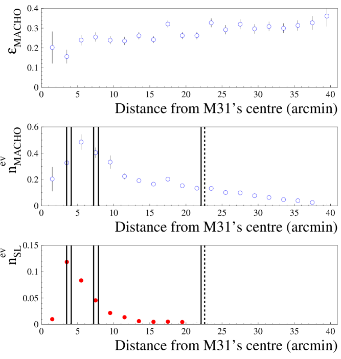
Figure 11: Predictions of the full simulation as a function of the distance from the centre of M31. Upper pannel: efficiency correction (for MACHOs); central panel: expected number of MACHO events (full halo, $M=0.5$ M_⊙, $a_{M31}=3\,{\mathrm{kpc}}$); bottom panel: expected number of self-lensing events (for a stellar bulge (disc) $M/L_{B}=3\,(4)$). The vertical lines indicate the position of the observed events, the dashed line corresponds to PA-00-S4, which has been excluded from the analysis because it is a probably M31/M32 intergalactic event.

.

	$\Delta\Theta<4^{\prime}$	$4<\Delta\Theta<8^{\prime}$	$\Delta\Theta>8^{\prime}$
mass (M⊙)
Halo, $a_{M31}$ = 3 kpc
1	$0.70\pm 0.12$	$1.38\pm 0.08$	$2.96\pm 0.04$
$5\cdot 10^{-1}$	$0.81\pm 0.17$	$1.93\pm 0.11$	$4.18\pm 0.08$
$10^{-1}$	$1.63\pm 0.32$	$3.00\pm 0.20$	$8.10\pm 0.23$
$10^{-2}$	$1.93\pm 0.45$	$3.85\pm 0.30$	$12.65\pm 0.29$
$10^{-3}$	$0.72\pm 0.27$	$2.20\pm 0.30$	$9.17\pm 0.29$
$10^{-4}$	$0.064\pm 0.042$	$0.60\pm 0.18$	$3.09\pm 0.18$
$10^{-5}$	$0.002\pm 0.002$	$0.034\pm 0.015$	$0.42\pm 0.06$
Halo, $a_{M31}$ = 5 kpc
1	$0.60\pm 0.10$	$1.11\pm 0.06$	$2.48\pm 0.04$
$5\cdot 10^{-1}$	$0.74\pm 0.18$	$1.57\pm 0.09$	$3.63\pm 0.09$
$10^{-1}$	$1.30\pm 0.25$	$2.52\pm 0.16$	$6.94\pm 0.12$
$10^{-2}$	$1.41\pm 0.34$	$3.63\pm 0.29$	$11.29\pm 0.24$
$10^{-3}$	$0.81\pm 0.30$	$2.07\pm 0.26$	$8.41\pm 0.26$
$10^{-4}$	$0.15\pm 0.15$	$0.49\pm 0.15$	$2.83\pm 0.16$
$10^{-5}$	$0.002\pm 0.002$	$0.048\pm 0.022$	$0.40\pm 0.05$
self lensing	$0.29\pm 0.02$	$0.29\pm 0.01$	$0.16\pm 0.01$

Table 8: The expected number of MACHO and of the self-lensing events, corrected for efficiency, for the models with $a_{M31}=3\,{\mathrm{kpc}}$ and $a_{M31}=5\,{\mathrm{kpc}}$, in three different ranges of distance from the M31 centre. The stellar bulge (disc) $M/L_{B}$ ratio is equal to $3\,(4)$.

In Table 8 we present the expected numbers of self-lensing and halo events (for a full halo and two different values of the core radius) predicted by the full simulation in the three distance ranges $\Delta\Theta<4^{\prime},\,4<\Delta\Theta<8^{\prime}$ and $\Delta\Theta>8^{\prime}$. The self-lensing results, given for a stellar bulge $M/L_{B}$ ratio equal to 3, are dominated by stellar bulge lenses and therefore scale with this ratio. This must be compared with the 5 microlensing events reported in Sect. 3. PA-00-S4, which is located near the line of sight toward the M32 galaxy, is likely an intergalactic microlensing event (Paulin-Henriksson et al. 2002) and therefore not included in the present discussion. Accordingly, we have excluded from the analysis a 4’ radius circular region centred on M32.

The main issue we have to face is distinguishing self-lensing events from halo events. This is particularly important as the number of expected MACHO and self-lensing events is of about the same order of magnitude if the halo fraction is of order 20% or less as in the direction of the Magellanic clouds.

	$a_{M31}=3$ kpc			$a_{M31}=5$ kpc
Mass (M⊙)	$f_{\mathrm{INF}}$	$f_{\mathrm{MAX}}$	$f_{\mathrm{SUP}}$	$f_{\mathrm{INF}}$	$f_{\mathrm{MAX}}$	$f_{\mathrm{SUP}}$
1	0.27	0.81	0.97	0.29	0.97	0.97
$5\cdot 10^{-1}$	0.22	0.57	0.94	0.24	0.67	0.96
$10^{-1}$	0.13	0.31	0.74	0.15	0.37	0.83
$10^{-2}$	0.08	0.21	0.51	0.09	0.23	0.57
$10^{-3}$	0.11	0.29	0.73	0.12	0.31	0.76
$10^{-4}$	0.20	0.77	0.96	0.18	0.81	0.96
$10^{-5}$	0.12	1.00	0.97	0.10	1.00	0.97

Table 9: Results for the halo fraction $f$: the 95% CL lower bound ($f_{\mathrm{INF}}$) and upper bound ($f_{\mathrm{SUP}}$), and maximum probability ($f_{\mathrm{MAX}}$) are displayed for $a_{M31}=3\,{\mathrm{kpc}}$ and $a_{M31}=5\,{\mathrm{kpc}}$. In both cases, the stellar bulge (disc) $M/L_{B}$ ratio is $3\,(4)$.

Although the observed characteristics of the light curves do not allow one to disentangle the two classes of events, the spatial distribution of the detected events (Fig. 1) can give us useful insights. While most self-lensing events are expected in the central region, halo events should be more evenly distributed out to larger radii. In Figure 11, together with the distance dependence of the detection efficiency, we show the expected spatial distribution of self lensing and 0.5 M_⊙ MACHO events (full halo). The observed events are clustered in the central region with the significant exception of PA-99-N2, which is located in a region where the self-lensing contamination to MACHOs events is expected to be small.

The key aspect of our analysis is the comparison of the expected spatial distribution of the events with that of the observed ones. In order to carry out this comparison as precisely as possible, we divide the observed field into a large number of bins, equally spaced in distance from M31’s centre. We present here an analysis with 20 bins of 2’ width, but we have checked that the results do not change significantly if we use either 40 bins of 1’ width or 10 bins of 4’ width.

6.1 The halo fraction

The first striking feature in the comparison between predictions and data is that we observe far more events than predicted for self lensing alone. Therefore, it is tempting to conclude that the events in excess with respect to the prediction should be considered as MACHOs. This statement can be made more quantitative: given a MACHO halo fraction, $f$, we can compute the probability of getting the observed number of events and, by Bayesian inversion, obtain the probability distribution of the halo fraction.

As already outlined, we bin the observed space into $N_{bin}$ equally spaced annuli and then, given the model predictions $x_{i}$ ($i=1\ldots N_{bin}$), obtain the combined probability of observing in each bin $n_{i}$ events. The combined probability is the product of the individual probabilities of independent variates $n_{i}$:

$$P\left(n_{i}|x_{i}\right)=\prod^{N_{bin}}_{i=1}\frac{1}{n_{i}!}\exp(-x_{i})x_{i}^{n_{i}}.$$ (6)

For a given a model, the different $x_{i}$ are not independent: they all depend on the halo fraction $f$ via the equations

$$x_{i}=h_{i}\,f+s_{i},$$ (7)

where $h_{i}$ and $s_{i}$ are the numbers of events predicted in bin $i$ for a full MACHO halo and self lensing, respectively. A model specifies $h$ and $s$, so the probability depends on only one parameter, $f$. It is therefore possible to evaluate lower and upper limits at a given confidence level for the halo fraction $f$.

In Figure 12 and Table 9, we display the 95% confidence level (CL) limits obtained in this configuration for $a_{M31}=3\,{\mathrm{kpc}}$ and $M/L_{B}=3$. We get a significant lower limit, $f_{\mathrm{INF}}>20\%$, in the mass range from 0.5 to 1 $M_{\odot}$. No interesting upper bound on $f$ is obtained except around a mass of $10^{-2}\,M_{\odot}$ ($f_{\mathrm{SUP}}=50\%$).

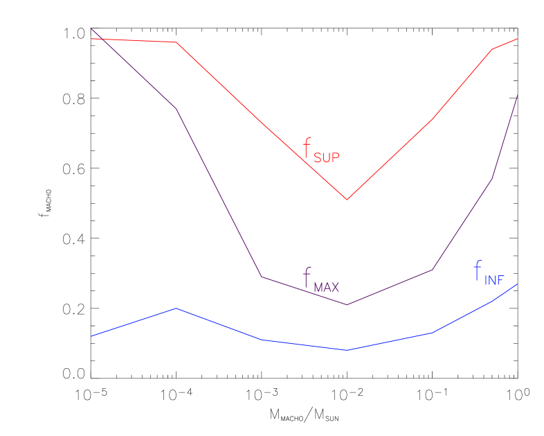
Figure 12: Most probable value, upper and lower 95% CL limit for the halo fraction as a function of the MACHO mass for $a_{M31}=3\,{\mathrm{kpc}}$ and stellar bulge (disc) $M/L_{B}=3\,(4)$.

We also show in Table 9 the same limits for $a_{M31}=5\,\mathrm{kpc}$. As the predicted halo contribution is smaller, the inferred lower limit on $f$ is slightly larger.

6.2 Self-lensing background ?

The fact that 4 out of the 5 observed events lie within 8’ from the centre of M31 could be suggestive of self-lensing origin, implying that we underestimate this contribution. However, in the Monte Carlo section we have already seen that the velocity dependence of our results is very weak. For models 2 (3), where the change is maximum, the 95% CL lower limit on $f$ in the mass range 0.1-1 M_⊙ is shifted by about - (+) 0.02. Furthermore, $M/L_{B}$ ratios larger than 4 cannot be accommodated by known stellar populations. Still, for comparison, we have considered models for which, on dynamical grounds, the $M/L_{B}$ ratio of either the disc or the bulge take values up to $\sim 8-9$. One can see from Table 10 that our conclusions are not qualitatively altered. This can be partly attributed to the occurence of PA-99-N2 $22^{\prime}$ away from the M31 centre.

Bulge ${M/L}_{B}$	Disc ${M/L}_{B}$	$n_{SL}$	$P(f=0)$	$f_{\mathrm{INF}}$
3	4	0.72	$10^{-4}$	0.22
3	9	1.1	$10^{-3}$	0.17
8	4	1.5	$4\,10^{-3}$	0.15

Table 10: For different sets of values of stellar bulge and disc $M/L_{B}$ (Sect. 4.1.2) we report the number of expected self-lensing events, corrected for the efficiency, the probability for the signal to be a Poisson fluctuation for a $f=0$ halo and, for a $M=0.5\,\mathrm{M}_{\odot}$ MACHO population MW and M31 halos with $a_{M31}=3\,\mathrm{kpc}$, the 95% CL lower bound for the halo fraction $f$.

One can also question the bulge geometry. However, we have seen that assuming a spherical bulge with the same mass and luminosity does not alter the results. One could also think of a bar-like bulge. This possibility has been considered by Gerhard (1986), who has shown that unless a would be bar points toward us within $10^{\circ}$, its ellipticity does not exceed 0.3. This cannot produce a significant increase of the self-lensing prediction. Even if a bar-like bulge points toward us and is highly prolate, it cannot explain event PA-99-N2.

Clearly, unless we grossly misunderstand the bulge of M31, our events cannot be explained by self lensing alone.

Still, in view of our low statistics, we could be facing a Poisson fluctuation. However, this is highly improbable: given the prediction of our simulation, the probability of observing 5 self-lensing events with the observed spatial distribution is $P(f=0)\sim 10^{-4}$ for a $M/L_{B}=3\,(4)$ M31 stellar bulge (disc), and remains well below $\sim 10^{-2}$ even for much heavier configurations (Table 10).

7 Conclusions

In this paper, we present first constraints on the halo fraction, $f$, in the form of MACHOs in the combined halos of M31 and MW, based on a three-year search for gravitational microlensing in the direction of M31.

Our selection pipeline, restricted to bright, short-duration variations, leads us to the detection of 6 candidate microlensing events. However, one of these is likely to be a M31-M32 intergalactic self-lensing event, so we do not include it when assessing the halo fraction $f$.

We have thoroughly discussed the issue of the possible contamination of this sample by background variable stars. Indeed, we are not aware of any class of variable stars able to reproduce such light curves, therefore we have assumed that all our candidates are genuine microlensing events.

To be able to draw physical conclusions from this result, we have constructed a full simulation of the expected results, which involves a Monte Carlo  simulation completed by an event simulation to account for aspects of the observation and the selection pipeline not included in the Monte Carlo.

The full simulation predicts that M31 self lensing alone should give us less than 1 event, whereas we observe 5, one of which is located $22^{\prime}$ away from the M31’s centre, where the expected self-lensing signal is negligible. As the probability that we are facing a mere Poisson fluctuation from the self-lensing prediction is very small ($\sim 0.01\%$), we consider these results as evidence for the detection of MACHOs in the direction of M31. In particular, for $a_{M31}=3\,\mathrm{kpc}$ and a $M/L_{B}$ ratio for the disc and stellar bulge smaller than 4, we get a 95% CL lower limit of $20-25\%$ for $f$, if the average mass of MACHOs lies in the range 0.5-1 $M_{\odot}$. Our signal is compatible with the one detected in the direction of the Magellanic clouds by the MACHO collaboration (Alcock et al. 2000).

We have also considered models that, on dynamical grounds, involve higher disc or stellar bulge $M/L_{B}$ ratios. However, because of the spatial distribution of the observed events, the conclusion would not be qualitatively different. Indeed, because of the presence of the event PA-99-N2 $22^{\prime}$ away from the M31 centre where self lensing is negligible, the lower bound on $f$ would not pass below $\sim 15\%$ even in the most extreme models considered.

Finally, the observed events can hardly be blamed on the geometry of the bulge. Indeed, the number of predicted self-lensing events cannot be significantly increased unless it has a highly prolate bar-like structure exactly pointing toward us. However, even this improbable configuration would not explain one of the events, which definitely occurs outside the bulge.

Beside the 5 events selected by our pipeline, we have found a very likely candidate for a binary lensing event with caustic crossing. This event occurs $\sim 32^{\prime}$ away from M31’s centre, where one can safely ignore self lensing. Therefore, although included in neither our selection pipeline nor our discussion on the halo fraction, this detection strengthens our conclusion that we are detecting a MACHO signal in the direction of M31.

To get more stringent constraints on the modelling of M31, better statistics are badly needed. To achieve this goal using our data, we plan to extend the present analysis in a forthcoming work by looking for fainter variations. Another option would be to lift the duration cut. However, we consider this less attractive, because the contamination by the background of variable stars would be much larger and difficult to eliminate. Moreover, the Monte Carlo predictions disfavour a major contribution of long duration events.

Note added in proof.

After submission of this work, the MEGA collaboration presented their results obtained independently from the same data (De Jong et al., [arXiv:astro-ph/0507286 v2]). Their conclusions are different from ours. We would like to point out that their criticism of our analysis is not relevant because, as stated in Section 4.1.2, we choose to only consider for self lensing evaluation a population of stars with a standard M/L ratio, which does not need to account for the total dynamical mass nor to reproduce the inner rotation curve.