ELT Observations of Supernovae at the Edge of the Universe

Abstract

We discuss the possibility of using Supernovae as tracers of the star formation history of the Universe for the range of stellar masses $\sim 3-30$ M_⊙ and possibly beyond. We simulate the observations of 350 SNe, up to $z\sim 15$, made with OWL (100m) telescope.

1 Introduction

The detection and the study of Supernovae (=SNe) is important for at least two reasons: 1. the use of local SNe (both type Ia and II) as ‘calibrated’ standard candles (Phillips 1993, Hamuy et al. 2001, Hamuy & Pinto 2002) provides a direct measurement of the expansion rate of the Universe H_∘, and their detection at $z>0.3$ allows to measure its deceleration parameter q_∘ and to probe different cosmological models (Perlmutter et al. 1998, 1999; Riess et al. 1998); 2. the evolution of the cosmic SN rate provides a direct measurement of the cosmic star formation rate (SFR). Indeed the rate of core-collapse SN explosions (SN II, Ib/c) is a direct measurement of the death of stars with masses in the range 8-30 M_⊙ (although it is still debated if stars more massive than 30 M_⊙ could make ”normal” type II/Ibc SNe, or rather collapse forming a BH with no explosion at all, or even make a different kind of explosion like GRBs; see, e.g., Heger et al. 2001). Similarly, type Ia SNe may provide the history of star formation of moderate mass stars, 3-8 $M_{\odot}$, i.e. their most likely progenitors provided that the SN Ia explosion process is unambiguously identified (e.g. Mannucci, Della Valle & Panagia 2005). In addition the evolution of the SN-Ia rate with redshift helps to clarify the nature of their progenitors (e.g. Madau, Della Valle & Panagia 1998, Dahlen et. al 2004, Strolger et al. 2004).

2 SNe as tracers of star formation

For a Salpeter Initial Mass Function (IMF) with an upper cutoff at 100 M_⊙ we find that half of all SNII is produced by stars with masses between 8 and 13 M_⊙ and half of the mass in SN-producing stars is in the interval of mass $\sim 8-22$ M_⊙. A main sequence star with 13 M_⊙ has approximately a luminosity of 8000 L_⊙ and a temperature of 22000 K and one with 22 M_⊙ has L$\sim 3.5\times 10^{4}L_{\odot}$ and T${}_{eff}\sim 27000$ K. This means that more than half of the SN producing stars are rather poor sources of ionizing photons and of UV continuum photons, while the bulk of the UV radiation, both in the Balmer and in the Lyman continuum is produced by much more massive stars. Actually, starburst models (e.g. Leitherer et al. 1999) suggest us that stars above 30 M_⊙ produce 90% of the Lyman continuum photons and 70% of the 912-2000Å  UV continuum. It follows that the bulk of the UV radiation both in the Balmer and Lyman continuum is produced by stars more massive than 30$M_{\odot}$, so that the H$\alpha$ and UV fluxes measure only the very upper part of the IMF (stars with masses $>30_{\odot}$ represent only 13% of the total number of stars with masses larger than $>8M_{\odot}$). Therefore, H$\alpha$ and UV flux are not ideal indicators of star formation rate because: a) they require a huge extrapolation to lower masses and b) the extrapolation depends on the value of minimum mass to make a SNII, M_up, which is not well known and may be different in different environments (Bressan et al. 2002) or at different redshifts (Heger et al. 2001). On the other hand, SNe can provide a measurement of the star formation rate which is: i) independent of other SFR determinations; ii) more direct because the IMF extrapolation is appreciably smaller; iii) more reliable because it is based on counting SN explosions rather than relying on identifying and measuring the sources of ionization or of UV continuum. A possible drawback for this approach is the fact that a significant fraction of SNe may be missed because of extinction in their parent galaxies (Mannucci et al. 2003).

3 The Ingredients of the Simulation

Our simulation is based on a number of assumptions:

1. ELT performance. We have assumed ELT= OWL, i.e. a 100m telescope. The imaging and spectroscopic limits are a function of the S/N ratio as derived from the ELT exposure time calculator (www-astro.physics.ox.ac.uk/ imh/ELT).

2. OWL field. A reasonable extrapolation of the current technological standards let us presume that diffraction limited observations of a $2^{\prime}\times 2^{\prime}$ field, corrected with adaptive optics (K band), is within the technological possibilities of the next decade (Ragazzoni, private communication).

3. Number of SNe expected in a single OWL frame. Based on the results obtained by Madau et al. (1998), Miralda Escudé & Rees (1997), Mackey et al. (2003) and Weinmann & Lilly (2005) we estimate an observed rate of up to 7 SNe/yr per OWL field. Here we are including the very powerful Pop III SNe that are expected to be produced by pair-creation in zero-metallicity massive stars, in the range $140-260M_{\odot}$ (Heger et al. 2001).

4. Spectral energy distribution (=SED) of SNe (see Fig. 1). We have assumed as templates for type Ia and II : SN 1992A, SN 1999em and SN 1998S (Panagia 2003, Riess et al. 2004). The SED for SNe originating from Pop III stellar population has been obtained from Heger et al. (2001).

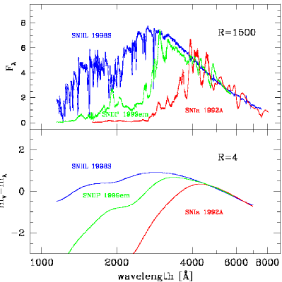
Figure 1: Spectral Energy Distribution adopted for type I and type II SNe. [Adapted from Panagia 2003]

5. Observational strategy. It is based on the control time methodology (Zwicky 1938). The morphology of the light curves and the absolute magnitudes at maximum of SNe have been obtained from Barbon, Ciatti & Rosino (1973), Dogget & Branch (1985), Patat et al. (1994) and Saha et al. (2001).

6. Distribution of SNe into spectroscopic types. These data have come from: Mannucci et al. (2004), Della Valle et al. (2005), Mackey et al. (2003), and Cappellaro et al. (1997). We have estimated about 63% of SNe to be of type II (a few SNe-II are expected to be observed during the UV shock breakout, that at z$\sim 7-8$ should last about 4-5 days in the observer rest frame), about 20% type Ia, 16% type Ib/c, and about 1% SNe from Pop III.

7. Cosmology ($\Omega_{m}=0.3$, $\Omega_{\Lambda}=0.7$) (e.g. Knop et al. 2003, Riess et al. 2004)

4 Redshift Thresholds

Fig. 2-5 represent the spectroscopic templates for SNeI-a, SNeII, and Pop III at different redshifts as viewed in the observer rest-frame. The three solid lines denote the fluxes, at different resolution factors, corresponding to S/N=10 for OWL exposures of $10^{5}$ sec. The dashed line is the threshold (R=5) for JWST (Panagia et al. 2003). Scaling the data in Figures 2-5 reveals that SNe are well detectable with OWL in 1h exposure. SNe-Ia are detectable up to $z\sim 5$ while SNe-II (bright) up to $z\sim 7-8$. Pop III SNe, which in principle would be easily detectable up to $z\sim 20$ (Heger et al. 2001) are unlikely observable beyond $z\sim 15$, due to the Lyman forest absorption.

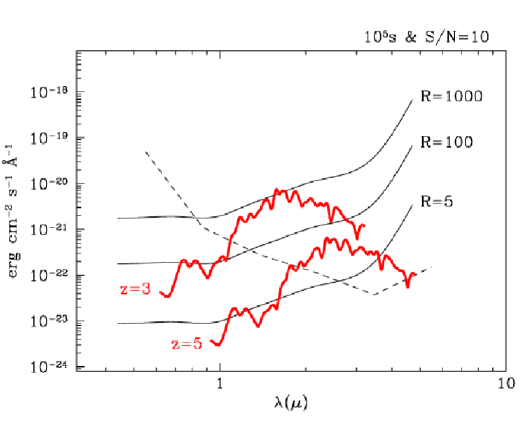
Figure 2: The spectroscopic template for type Ia SNe as viewed in the rest-frame of the observer, at different redshifts. The three solid lines denote the fluxes corresponding to a S/N=10 for OWL exposures of $10^{5}$ s at different resolutions. The dashed line is the threshold (R=5) for JWST.

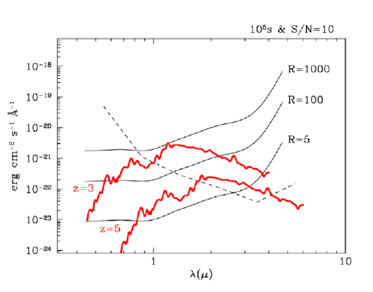
Figure 3: The same as Fig. 2 for SNe-II (regular).

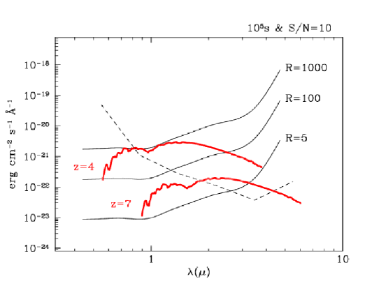
Figure 4: The same as Fig. 2 for SNe-II (bright).

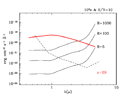
Figure 5: The same as Fig. 2 for SNe originating from Pop III stellar population. The template has been derived from Heger et al. 2001 (their Fig. 3).

5 The Simulation

An ELT project devoted to the study the evolution of the cosmic SN rate up to $z\sim 15$ requires an important (although not huge, as we shall see) investment of telescope time. We plan to carry out the SN search on 50 OWL fields in the J, H and K bands (1 hour each) at 4 different epochs over an interval of time of 1 year. This strategy is justified by the following considerations. The typical light curve width around maximum light is 15-20 days in the SN rest frame, and most SNe will occur at $z<5$ (see Fig. 2-5). Therefore, the light curve widths in the observer rest frame correspond to about 100-120 days, so that 4 exposures obtained 3 months apart will cover all events occurring within 1 year. In addition we need 3 more epochs (1h each) in the K band for the photometric follow-up and 1 spectroscopic epoch (4h for each SN discovered at $z<5$) for the spectroscopic classification. At very high redshifts, z $\sim 7-8$, only bright type II SNe may be used as standard candles (due to their strong UV emission, while SNe Ia are basically blind below $2400\AA$  and therefore they are detectable ‘only’ up to z$\sim 5$). Bright type II SNe can be standardized via “expanding photosphere method” (Hamuy et al. 2001) or alternatively via expansion velocity vs. bolometric luminosities relationship at the plateau stage (Hamuy & Pinto 2002). This task can be accomplished by securing a second and possibly a third spectroscopic epoch, and this requires about 200 hours of observing time. Finally, we need 4h for each Pop III SN to obtain medium/high resolution spectroscopy.

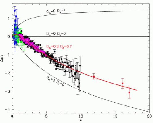
Figure 6: Hubble diagram for the simulated ELT observations of SNe. Pink, black and red dots represent type Ia, type II (+Ib/c) SNe and SNe from Pop III stellar population. Blue and green dots are ‘real’ SNe observed with ground based telescopes and HST, respectively.

In summary, this programme requires a “grand total” of 1270h, of which 600h are for the SN search, 150h for the photometric follow-up (K band) and 200h for the spectroscopy of type Ia, Ib/c and II SNe, 200 additional hours for the second and third spectroscopic epochs of bright type II SNe and finally 120h for the spectroscopy of Pop III SNe. All of this corresponds to about 160 nights, which will allow us to study about 350 SNe. This is certainly an important investment in terms of telescope time, however we note that this corresponds to about three times as much the size of a current HST Treasury programme (450 orbits) and it is comparable with the requirements of the SNAP (now Joint Dark Energy Mission) project, which is expected to study about 2000 SNe Ia (at $z<2$) in 2 years (Aldering et al. 2002). In Fig. 6 we show the ‘virtual’ SNe discovered by OWL: pink dots are type Ia SNe, black dots type II (+Ib/c), blue and green dots are Ia SNe ‘actually’ discovered by ground based telescopes (Perlmutter 1998, 1999; Riess 1998; Knop et al. 2003, Tonry et al. 2003) and from HST (Riess et al. 2004). The SNe have been distributed around the track $\Omega_{m}=0.3$, $\Omega_{\Lambda}=0.7$ after taking into account the intrinsic dispersion of the peak of the luminosity of type Ia and II SN populations, while the photometric errors have been derived from the S/N ratio that has been computed for each simulated observation. Red dots represent SNe from Pop III star population. The explosion rate for Pop III SNe was taken from Mackey et al. (2003). However, recently Weinmann & Lilly (2005) found that this rate may be too high and it should be decreased by an order of magnitude. In this paper we assume as an estimate of the rate of Pop III SNe (up to z$\sim 15$) in the $2\times 2$ arcmin² OWL field: R${}_{SNe-III}\simeq f\times d\times 5\times 10^{-2}$/yr SNe, being $f$ an efficiency factor ranging between 1 (Mackey et al. 2003) and 0.1 (Weinmann & Lilly 2005) and $d$ the duration (in years) of the SN peak. According to Heger et al. (2001, their Fig. 3) $d$ is about 1 (at 2-3$\mu$, in the observer rest-frame) therefore, one should be capable to observe during the OWL survey about $f\times 5\times 10^{-2}\times 50$ fields $\simeq f\times 3$ SNe at any time.

6 Conclusions

In this paper we have argued that SNe can be used as profitable tracers of cosmic star formation for a number of reasons: i) the determinations of the SFR based on SN measurements are independent of other possible determinations, ii) SNe provide a more direct diagnostics than the UV luminosity or the H$\alpha$ line emission because the IMF extrapolation is much smaller and iii) SNe are a more reliable source of information because it is based on a simple count of individual SN explosions rather than relying on identifying and measuring the source of ionization (if using H-alpha flux) or the source of UV continuum. In addition, by studying SNe at high redshifts iv) we can learn to what extent the IMF was more skewed toward massive stars (relatively to a normal Salpeter’s) in low metallicity environments, and v) we can study the properties of the progenitors of the primordial Gamma Ray Bursts (=GRBs) (given the growing evidence for the existence of an association between core collapse SNe with the long duration GRBs, see Della Valle 2005 and references therein).

The results of our simulation indicate that $\sim 350$ SNe can be studied up to $z\sim 15$ within a reasonable amount of telescope time (about 160 nights). This pilot programme has been conceived to study the history of the cosmic star formation rate, nevertheless a number of important by-products are at hand: such as vi) to disentangle cosmological models alternative to $\Lambda$, vii) to clarify the nature of the progenitors of type Ia SNe viii) to probe the physical properties of the ISM and IGM at $z>10$ through high spectral resolution (R$\sim 10^{4}$) of Pop III SNe (feasible with 50–100m telescope) ix) to explore the metal enrichment of the IGM at early epochs (up to $z\sim 4$) via observations of bright type II and Ia SNe at a resolution of $R\sim 1000$ (feasible with 50-100m telescope).

References

- (1) Aldering et al. 2002, SPIE 4835 ()
- (2) Barbon, R., Ciatti, F., & Rosino, L. 1973, A&A, 25, 241
- (3) Bressan, A., Della Valle, M., Marziani, P. 2002, MNRAS, 331, L25
- (4) Cappellaro, E., Turatto, M., Tsvetkov, D. Yu., Bartunov, O. S., Pollas, C., Evans, R., Hamuy, M. 1997, A&A, 322, 431
- (5) Dahlen et al. 2004, ApJ, 613, 189
- (6) Della Valle, M. et al. 2005, ApJ, in press
- (7) Della Valle, M. 2005, in the Proceedings of the ”Gamma-Ray Bursts in the Afterglow Era: 4th orkshop”, Rome, 2004.
- (8) Doggett, J. B., Branch, D. 1985, AJ, 90 2303
- (9) Hamuy, M. et al. 2001, ApJ, 558, 615
- (10) Hamuy, M., & Pinto, P.H. 2002, ApJ, 566, L63
- (11) A. Heger, S. E. Woosley, I. Baraffe, T. Abel 2001 in. proc. MPA/ESO/MPE/USM Joint Astronomy Conference ”Lighthouses of the Universe: The Most Luminous Celestial Objects and their use for Cosmology” (astro-ph/0112059)
- (12) Knop, R. A, et al., 2003, ApJ, 598, 102.
- (13) Leitherer, C. et al. 1999, ApJS, 123, 3
- (14) Madau, P., Della Valle, M., Panagia, N. 1998, MNRAS, 297, L17
- (15) Mannucci, F. et al. 2003, A&A, 401, 519
- (16) Mannucci, F. et al. 2005., A&A, 433, 807
- (17) Mannucci, F., Della Valle, M., & Panagia, N., 2005, in preparation
- (18) Miralda-Escudé, J. & Rees, M. 1997, ApJ, 478, L57
- (19) Mackey, J., Bromm, V., Hernquist, L. 2003, ApJ, 586, 1
- (20) Panagia, N., 2003, in “Supernovae and Gamma-Ray Bursters”, ed. K. W. Weiler (Springer-Verlag), p. 113-144.
- (21) Panagia, N., Stiavelli, M., Ferguson, H.C., & Stockman, H.S., 2003, in ”Galaxy Evolution: Theory and Observations”, eds. V. Avila-Reese, C. Firmani, C.S. Frenk, & C. Allen, RevMexAA SC, 17, p. 230-234.
- (22) Patat, F., Barbon, R., Cappellaro, E., Turatto, M. 1994, A&A, 282, 731
- (23) Phillips, M.M. 1993, ApJ, 413, L105
- (24) Perlmutter, S. et al. 1998, Nature, 391, 51
- (25) Perlmutter, S. et al. 1999, ApJ, 517, 565
- (26) Riess, A. et al. 1998, AJ, 116, 1009
- (27) Riess, A. et al. 2004, ApJ, 607, 665
- (28) Saha, A. et al. 2001, ApJ, 551, 973
- (29) Strolger, L.G. et al. 2004, ApJ, 613, 200
- (30) Tonry, J.L. et al. 2003, ApJ, 594, 1
- (31) Weinmann & Lilly 2005, ApJ, in press, astro-ph/0412248
- (32) Zwicky, F. 1938, ApJ 88, 529