Predicting Single-Temperature Fit to Multi-Component Thermal Plasma Spectra

Abstract

Observed X-ray spectra of hot gas in clusters, groups, and individual galaxies are commonly fit with a single-temperature thermal plasma model even though the beam may contain emission from components with different temperatures. Recently, Mazzotta et al. pointed out that thus derived $T_{\text{spec}}$ can be significantly different from commonly used definitions of average temperature, such as emission- or emission measure-weighted $T$, and found an analytic expression for predicting $T_{\text{spec}}$ for a mixture of plasma spectra with relatively hot temperatures ($T\gtrsim 3$ keV). In this Paper, we propose an algorithm which can accurately predict $T_{\text{spec}}$ in a much wider range of temperatures ($T\gtrsim 0.5$ keV), and for essentially arbitrary abundance of heavy elements. This algorithm can be applied in the deprojection analysis of objects with the temperature and metallicity gradients, for correction of the PSF effects, for consistent comparison of numerical simulations of galaxy clusters and groups with the X-ray observations, and for estimating how emission from undetected components can bias the global X-ray spectral analysis.

1. Introduction

Temperature of the hot gas filling the volume of galaxy clusters and groups is the primary diagnostic of properties and physical processes in these objects. An incomplete list of applications includes the study of radiative cooling and feedback mechanisms in the cluster centers; distribution of heavy elements in the intracluster (ICM) and interstellar (ISM) media; estimation of the cluster mass either through the virial $M-T$ relation or application of the hydrostatic equilibrium equation (e.g., Evrard et al., 1996; Sarazin, 1988; Mathews, 1978).

ICM temperature is usually measured by fitting its observed X-ray spectrum. Generally, the spectrum is integrated within a beam which contains several components with different $T$ and metallicity. Current detectors, such as CCDs onboard Chandra and XMM-Newton, cannot spectrally separate emission from different components. Also, statistical quality in the vast majority of cases is insufficient to detect the presence of several emission components in the total spectrum. Therefore, single-temperature models are commonly fit to the integrated spectrum with the hope that the derived $T$ is a representative average of the temperatures within the beam.

Recently, Mazzotta et al. (2004) pointed out that the temperature derived from the X-ray spectral analysis, $T_{\text{spec}}$, is significantly different from commonly used averages, such as the emission measure-weighted $T_{EM}$ (volume-averaged with weight $w=\rho^{2}$), or emission-weighted $T_{E}$ ($w=\rho^{2}\,\Lambda(T)$, where $\Lambda(T)$ is the plasma emissivity per unit emission measure). The “spectroscopic” temperature is biased towards lower-temperature components and it is generally lower than either of $T_{E}$ or $T_{EM}$.

As discussed below, $T_{\text{spec}}$ depends not only on the input spectrum but also on the energy dependence of the effective area of the X-ray telescope. However, Mazzotta et al. (2004) were able to find a simple analytic weighting scheme which predicts $T_{\text{spec}}$ for a known distribution of plasma temperatures and is sufficiently accurate for both Chandra and XMM-Newton, as long as the minimum temperature is sufficiently high, $T_{\text{min}}\gtrsim 3$ keV. This work can be applied (Mazzotta et al., 2004) for realistic comparison of the cluster numerical simulations and observations, for estimating detectability of hydrodynamic phenomena (shocks) in the X-ray data, for modeling the 3D distributions in the presence of temperature gradients, and for estimating how the presence of undetectable components can bias the global cluster properties inferred from the X-ray analysis (Rasia et al., 2005).

Unfortunately, the weighting scheme of Mazzotta et al. (2004) can be applied only for relatively high temperatures, $T_{\text{min}}\gtrsim 3$ keV, because it was developed for continuum-dominated spectra. It is important to be able to accurately predict $T_{\text{spec}}$ in the lower-temperature regime. For example, many of the cool clumps within the clusters, whose presence biases the global $T_{\text{spec}}$, probably have temperatures typical of galaxy groups or individual galaxies, $T\sim 1-2$ keV (Motl et al., 2004; Nagai et al., 2003; Dolag et al., 2004). Another application is in the analysis of the cluster regions outside half the virial radius where the ICM temperature drops below 50% of its peak value near the center (see Vikhlinin et al. 2005 for recent results on the cluster temperature profiles). An algorithm to predict $T_{\text{spec}}$ for low-temperature plasmas is required for the X-ray analysis of low-mass clusters, the objects which will provide the bulk of cosmological constraining power in the forthcoming Sunyaev-Zeldovich effect surveys (Haiman et al., 2001).

In this Paper, we develop an algorithm which accurately predicts $T_{\text{spec}}$ in the entire range of X-ray temperatures ($T\gtrsim 0.5$ keV), and for nearly arbitrary range of plasma metallicities. The algorithm is successful because it explicitly accounts for the low-energy line emission as the primary temperature diagnostics for low-$T$ plasmas. The general plan is as follows. In § 2, we briefly review how temperature is derived from the X-ray spectral analysis. Extreme cases of purely line-dominated and continuum-dominated spectra are considered in § 3. Spectroscopic temperature for in the case of realistic metallicities, $Z=0.1-2$ Solar, can be predicted using the results for these extreme cases, as discussed in § 4.

2. X-Ray Spectral Analysis

Before proceeding to discussion of the temperature-averaging techniques, we briefly review some technical aspects of the ICM temperature determination by current X-ray telescopes. X-ray spectrum of plasma enriched by heavy elements is superposition of continuum bremsstrahlung and emission lines. Advanced codes exist which can compute spectra of collisional-dominated plasma in a broad range of temperatures and metallicites: the Raymond-Smith model (Raymond & Smith, 1977), MEKAL (Mewe et al., 1985; Kaastra & Mewe, 1993; Liedahl et al., 1995), and APEC (Smith et al., 2001). We use the MEKAL model in this Paper; the results for other codes should be nearly identical.

Observed spectrum is significantly distorted because of the energy-dependent effective area of the X-ray telescopes and finite detector spectral resolution. For rigorous mathematical model of the instrumental response to input spectra, see Davis (2001). X-ray CCDs of the ACIS camera onboard Chandra and EPIC onboard XMM-Newton have a $\sim 100$ eV energy resolution (FWHM). Individual emission lines are blended when observed with such resolution and line and continuum emission at low energies cannot be fully separated (Fig.1).

Since it is impossible to reconstruct the input spectrum directly, its parameters are determined from fitting a model to the observed spectrum. Typically, the free parameters are the overall normalization, temperature, and abundance of heavy elements. The most temperature-sensitive features in the observed spectrum are the location of high-energy exponential cutoff in the continuum, if the temperature is sufficiently low so that the cutoff is within the instrument bandpass; the overall slope of the continuum emission; the location of the low-energy emission line complex (see below). The best-fit model tends to describe the most statistically significant of these features. Which feature takes precedence is determined by both the input spectrum and instrument characteristics such as relative sensitivity at low and high energies, the instrument bandpass, and the background. Therefore, different instruments will, generally, measure different $T$ if the input spectrum consists of multiple temperature components.

Figure 1.— Top: Observed Chandra spectrum of a $T=0.8$ keV galaxy group USGC S152. Histogram shows the MEKAL model spectrum convolved with the detector response. Bottom: Model spectrum binned into 10 eV energy channels.

In this paper, we focus on the single-temperature fits with free abundance of heavy elements, performed with the Chandra back-illuminated (BI) CCDs in the 0.7–10 keV energy band. We then show that the results are nearly identical in the same energy band for the Chandra front-illuminated (FI) CCDs, and only slightly different for the XMM-Newton and ASCA detectors (§ 5). More serious modifications will be required for very different instrumental setup, e.g. for high-resolution X-ray spectrometers or very different energy bands.

3. $T_{\text{spec}}$ In Extreme Cases

3.1. Average Temperature from Fitting Emission Lines

Ionization states of heavy elements and ion excitation rates sensitively depend on the plasma temperature. This makes the relative strengths of emission lines an attractive temperature diagnostics (Sarazin & Bahcall, 1977). The brightest lines in the typical ICM and ISM spectra are those of O VII and O VIII at $E\sim 0.6$ keV for $T\lesssim 0.5$ keV, the iron L-shell complex at $E\sim 1$ keV for $T=0.5-3$ keV, and Fe XV and Fe XVI lines at 6.7 and 6.95 keV for $T>3$ keV. In practice, the high energy Fe lines are not important for temperature determination because at the relevant temperatures, the spectrum is continuum-dominated. The Fe L-shell complex and O VII and O VIII lines, on the contrary, are very important because the plasma emission at low temperatures is line-dominated for commonly found metallicities ($Z\gtrsim 0.1$ Solar).

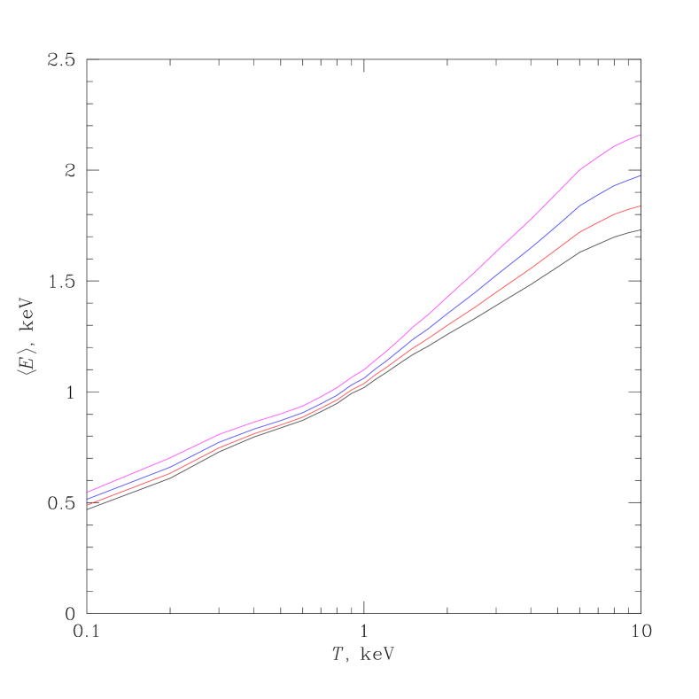
Figure 2.— Average energy for emission lines in the MEKAL spectra convolved with the Chandra BI response, as a function of plasma temperature. The lines from bottom to top are for $N_{H}=0$, $4\times 10^{20}$, $10^{21}$, and $2\times 10^{21}$.

Figure 3.— Single-temperature fits to line-dominated spectra. The input spectra consist of two components with temperatures $T_{\text{min}}$ and $T_{\text{max}}$, and with relative emission measures $f_{\text{min}}$ and $(1-f_{\text{min}})$. Left: results for $(T_{\text{min}},T_{\text{max}})=(0.25,0.5)$, $(0.5,1)$, and $(1,2)$ keV. Right: results for mixtures of 0.5 and 1.5 keV, and 1 and 3 keV components. On both panels, points show $T$ for a single-temperature fit to the simulated spectra. Solid line shows predictions of eq.[1–3]. Dotted lines correspond to naïve weighting, $\langle T\rangle=f_{\text{min}}\,T_{\text{min}}+(1-f_{\text{min}})\,T_{\text{max}}$.

The individual iron L-shell lines are not resolved by X-ray CCD detectors and the complex is observed as a single broad bump in the spectrum (Fig.1). As the plasma temperature increases, the complex is shifted towards higher energies. In fact, its location is the strongest temperature diagnostics in the low-$T$ regime. This suggests the following proposition: when a single-temperature model is fit to the line-dominated spectrum, the best-fit $T$ is such that the average energy in the input and model spectra are equal. The average energy can be defined as

$$\langle E\rangle=f(T)=\frac{\sum E_{i}\,s_{i}}{\sum s_{i}},$$ (1)

where $s_{i}$ is the observed count rate in channel $i$ and $E_{i}$ is the nominal energy corresponding to this channel. The count rates $s_{i}$ depend on the temperature, interstellar absorption, and detector sensitivity as a function of energy. Figure 2 shows $\langle E\rangle$ as a function of temperature assuming that the observation is performed with the Chandra BI CCDs.

Obviously, the average energy for a mixture of components with total count rates $S_{j}$ and temperatures $T_{j}$ is given by

$$\langle E\rangle_{\text{tot}}=\frac{\sum S_{j}\,f(T_{j})}{\sum S_{j}}.$$ (2)

The proposition formulated above implies that a single-temperature fit to the combined spectrum can be predicted by inverse function of eq. [1],

$$T_{\text{fit, lines}}=f^{-1}(\langle E\rangle_{\text{tot}}).$$ (3)

The functions $\langle E\rangle=f(T)$ can be pre-computed and tabulated and then eq. [3] provides an easy and fast method for predicting $T$ for a single-temperature fit.

The accuracy of this technique can be tested by direct XSPEC (Arnaud, 1996) simulations (Fig. 3). The single-$T$ fit can be accurately predicted for a mixture of 2 components with different temperatures as long as the dynamical range is not too large, $T_{\text{max}}/T_{\text{min}}\lesssim 2$. For larger temperature differences, predictions become less accurate because the emission complexes are well-separated and the composite spectrum is bimodal. The best fit in this case tends to model the brighter component and ignore the weaker one. Still, eq. [1–3] provide qualitatively correct predictions for the single-temperature fit which are much more accurate than weighting by emission measure (right panel in Fig.3). In more realistic cases, the temperature is distributed continuously between $T_{\text{min}}$ and $T_{\text{max}}$. The composite spectrum then will be unimodal and predictions for $T_{\text{fit}}$ should be quite accurate even when $T_{\text{max}}/T_{\text{min}}$ is large.

3.2. Average Temperature for Purely Continuum Spectra

Let us now consider the opposite case of spectra with zero metallicity. Predictions for the single-temperature fit to the continuum-dominated spectra were recently derived by Mazzotta et al. (2004). Mazzotta et al. noted that the spectrum of the high-temperature bremsstrahlung can be approximated by a linear law, $s(E)\approx a(T)-b(T)E$, within the limited bandpass of Chandra and XMM-Newton and this leads to the following weighting scheme for computing the average temperature,

$$\langle T\rangle=\frac{\int_{V}w\,T\,dV}{\int_{V}w\,dV},$$ (4)

where

$$w=\rho^{2}\,T^{-\alpha},\qquad\alpha\simeq 0.75.$$ (5)

Mazzotta et al. demonstrated that this formula is remarkably accurate for both Chandra and XMM-Newton, as long as all temperatures are sufficiently high, $T\gtrsim 3.5$ keV.

We would like to extend the weighting scheme [4] into the lower temperature regime. The obvious problem here is that the weights [5] are strongly skewed towards lower-temperature components. For $T\rightarrow 0$, $w\rightarrow\infty$ but in reality it should become zero because the spectrum is shifted below the bandpass of the X-ray detectors. A heuristic modification of eq. [5] could then be

$$w=c(T)\,\rho^{2}\,T^{-\alpha},$$ (6)

where $c(T)$ is the detector sensitivity to bremsstrahlung spectra characterized by the observed photon count rate within the energy band of interested for a spectrum with unit emission measure. For $T\rightarrow 0$, $c(T)\rightarrow 0$ and thus suppresses the weights for the low-temperature components.

Surprisingly, we find that eq. [6] with $\alpha=0.875$ works accurately in a very broad temperature range. The results of XSPEC simulations for mixtures of two components with $T_{\text{max}}/T_{\text{min}}=4$ and $T_{\text{min}}=0.25$, 0.5, 1, 2, and 4 keV are shown in Fig.4. The approximations by eq. [4,6] are shown by the solid lines. They are accurate in these cases to within $\Delta T<0.15$ keV or $\Delta T/T<4\%$, whichever smaller. Approximations using eq. [5] (dotted lines) are equally accurate at high temperatures but fail for $T\lesssim 2$ keV, as Mazzotta et al. (2004) warned.

The drawback of our modification of the Mazzotta et al. weighting scheme is that it is no longer purely analytic. The function $c(T)$ should be pre-computed and tabulated because it is unique for each observation setup, which includes the telescope effective area as function of energy, Galactic absorption, and energy range used for spectral fits. Since the setup can be quite arbitrary, $c(T)$ should be implemented as a computer code. However, the gains in accuracy and temperature range warrant these complications.

Figure 4.— Single-temperature fits to continuum-dominated spectra consisting of two components with temperatures $T_{\text{min}}$ and $T_{\text{max}}$, and with relative emission measures $f_{\text{min}}$ and $(1-f_{\text{min}})$. Simulations were performed for Chandra BI CCDs and for $(T_{\text{min}},T_{\text{max}})=(0.25,1)$, $(0.5,2)$, $(1,4)$, $(2,8)$, and $(4,16)$ keV. Filled circles show best-fit $T$ for a single-temperature model fit in the 0.7–10 keV energy band. Approximations for $T_{\text{spec}}$ using (4,6). Approximations using eq. [5] are shown by dotted lines for comparison.

4. $T_{\text{spec}}$ for spectra with typical metallicities

Thermal emission of ICM and ISM with typical metallicities, $Z=0.1-1$ Solar, is usually not purely line- or continuum-dominated. To predict the single-temperature fit for such metallicities, we need to find a valid combination of results for the extreme cases considered above.

A possible approach is suggested by results of XSPEC simulations shown in Fig. 5. The filled circles in this Figure correspond to single-temperature fits to mixtures of $T=1$ and $3$ keV spectra with metallicities of $Z=0.1$ Solar, and of $T=2$ and $6$ keV with $Z=0.3$ Solar. The approximations for the line-dominated ($Z\rightarrow\infty$) and continuum-dominated ($Z=0$) regimes derived in § 3 are shown by dotted and dashed lines, respectively. For both cases, $T_{\text{line}}<T_{\text{cont}}$ and the real single-temperature fit, $T_{\text{spec}}$, is between these two regimes. Also note that $T_{\text{spec}}$ approaches $T_{\text{line}}$ for large values of $f_{\text{min}}$, when the contribution of the line emission to the total count rate becomes more significant. The total spectrum is more continuum-dominated for small values of $f_{\text{min}}$, and we observe that $T_{\text{spec}}$ approaches $T_{\text{cont}}$. This suggests that the parameter $x$,

$$x=\frac{T_{\text{spec}}-T_{\text{line}}}{T_{\text{cont}}-T_{\text{line}}},$$ (7)

should depend on the relative contribution of the line and continuum emission to the total flux in the energy band used for spectral fitting.

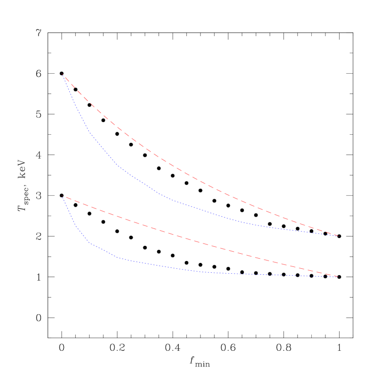
Figure 5.— Single-temperature fits to spectra with realistic metallicities. The input spectra have temperatures of 1 and 3 keV and metallicity $Z=0.1$ Solar (lower curves), and $T=2$ and 6 keV and $Z=0.3$ Solar (upper curves). Filled circles show best-fit $T$ for a single-temperature model fit in the 0.7–10 keV energy band. Approximations for continuum- and line-dominated spectra (see § 3) are shown by dashed and dotted lines, respectively.

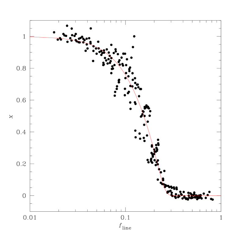
Figure 6.— The values of parameter $x$ in eq. [7] as a function $f_{\text{line}}$, fraction of the line emission in the total flux in the 0.7–10 keV energy band. Data points were obtained from XSPEC simulations spanning a wide range of temperatures, $T_{\text{max}}/T_{\text{min}}=2$, 3, and 4, $T_{\text{min}}=0.5$, 1, 2, and 3, and metallicities of 0.1, 0.3, and 1 Solar. Solid line shows analytic approximation of eq.[8].

We have performed a large number of XSPEC simulations of two-component spectra for a wide range of $T_{\text{min}}$, $T_{\text{max}}$, and metallicites. Figure 6 shows the values of parameter $x$ as a function of $f_{\text{line}}$, fraction of the line emission in the total flux in the 0.7–10 keV energy band which we use for spectral fitting. The data points in this Figure were derived from simulations with $T_{\text{max}}/T_{\text{min}}=2$, 3, and 4, $T_{\text{min}}=0.5$, 1, 2, and 3, and metallicities of 0.1, 0.3, and 1 Solar. Even though these cases probe very different regimes, all $x$ seem to follow a nearly universal function, which can be approximated as

$$x=\exp\left(-\frac{f_{\text{line}}^{2\beta}}{\Delta_{1}^{2\beta}}\right)\;\exp\left(-\frac{f_{\text{line}}^{8}}{\Delta_{2}^{8}}\right)$$ (8)

with $\beta=1$, $\Delta_{1}=0.19$, and $\Delta_{2}=0.25$ (solid line). As expected, $x\rightarrow 1$ and $T_{\text{spec}}\rightarrow T_{\text{cont}}$ for $f_{\text{line}}\rightarrow 0$, and $x\rightarrow 0$ and $T_{\text{spec}}\rightarrow T_{\text{line}}$ for $f_{\text{line}}\rightarrow 1$. The transition between the two regimes occurs for $f_{\text{line}}\simeq 0.2$. Apparently, emission lines at this point become the strongest feature in the observed spectrum and therefore they are the main driver for the single-temperature fit.

To further test the universality of eq. [8] we performed simulations for different values of Galactic absorption, $N_{H}=0$, $10^{20}$, $5\times 10^{20}$ and $2\times 10^{21}$ cm^-2. The values of $x$ obtained from these simulations were within the scatter of the data points in Fig. 6. This shows that at least for the same instrument setup (effective area and energy band of the spectral fit), the prescription for combining continuum- and lines-based temperatures is universal. Therefore, to properly combine $T_{\text{cont}}$ and $T_{\text{line}}$, we need to know only the fraction of the line emission in the total flux, $f_{\text{line}}(T)$, a quantity which is easy to pre-compute and tabulate.

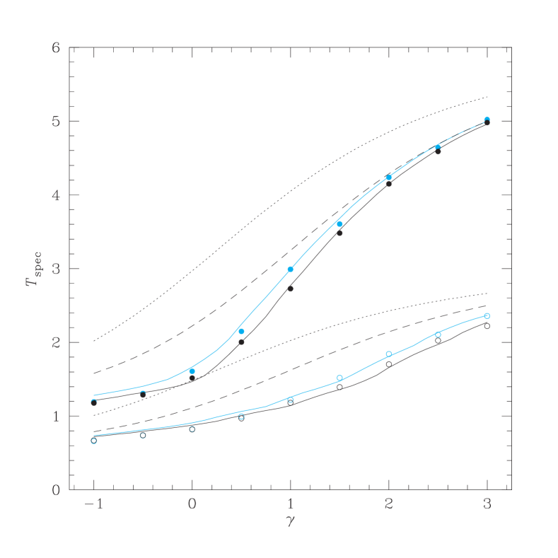
Figure 7.— Single-temperature fits to multiple-component spectra with $T$ distributed between $T_{\text{min}}$ and $T_{\text{max}}$ and emission measure $V\rho^{2}\propto T^{\gamma}$ (see text). Filled and empty circles show the simulation results for $T_{\text{min}}=1$ keV and $T_{\text{max}}=6$ keV, and for $T_{\text{min}}=0.5$ keV and $T_{\text{max}}=3$ keV, respectively. Approximations using the algorithm summarized in § 4.1 are shown by solid lines. Temperatures weighted by emission measure and using eq. [5] are shown by dotted and dashed lines, respectively. Blue points show the temperatures measured by the XMM-Newton EPIC-pn detector for the same input spectra, and blue solid line are the predictions of our model for this detector.

4.1. Putting It All Together: The Algorithm

To efficiently implement the method outline above, the following functions should be pre-computed and tabulated:

$c(T)$ — observed photon count rate for purely continuum spectra with unit emission measure, as a function of temperature;

$\lambda(T)$ — observed photon count rate for line emission for spectra with unit emission measure and Solar metallicity;

$\langle E\rangle=f(T)$ — average energy of the line emission (eq. [1]).

The continuum-based temperature for the composite spectrum, $T_{\text{cont}}$, is obtained using eq. [4,6] and the total continuum flux is given by the integral

$$F_{\text{cont}}=\int c(T)\,\rho^{2}\,dV.$$ (9)

The total flux and mean energy of the line emission are given by

$$F_{\text{line}}=\int\lambda(T)\,Z\,\rho^{2}\,dV,$$ (10)

$$\langle E\rangle=F_{\text{line}}^{-1}\int f(T)\,\lambda(T)\,Z\,\rho^{2}\,dV,$$ (11)

where $Z(x,y,z)$ is the metallicity distribution. The line-based temperature, $T_{\text{line}}$, is given by eq. [3]. To properly combine $T_{\text{cont}}$ and $T_{\text{line}}$, we first compute the fraction of the line emission in the total observed flux, $f_{\text{line}}=F_{\text{line}}/(F_{\text{line}}+F_{\text{cont}})$, then find the value of $x$ from eq. [8], and finally compute the spectroscopic-like temperature as

$$T_{\text{spec}}=x\,T_{\text{cont}}+(1-x)\,T_{\text{line}}.$$ (12)

To test how this scheme works in realistic cases, we performed XSPEC simulations for five-component spectra with temperatures equally log-spaced between $T_{\text{min}}$ and $T_{\text{max}}$,

$$T_{i}=T_{\text{min}}\left(T_{\text{max}}/T_{\text{min}}\right)^{i/4},\quad i=0,1,2,3,4,$$ (13)

and emission measures distributed as a power law of temperature,

$$V_{i}\,\rho_{i}^{2}\propto T_{i}^{\gamma}.$$ (14)

The relative contribution of the low- and high-temperature components to the overall spectrum is controlled by the value of index $\gamma$, which we vary in the range from $\gamma=-1$ to $\gamma=3$. Results of XSPEC simulations for such complex spectra are shown in Fig. 7. The results of single-temperature fits in the case of $T_{\text{min}}=0.5$ keV and $T_{\text{max}}=3$ keV, and $T_{\text{min}}=1$ keV and $T_{\text{max}}=6$ keV are shown by open and filled circles, respectively. Solid lines show the predicted values of $T_{\text{spec}}$. Clearly, we are able to predict the single-temperature fit very accurately. The residuals in Fig. 7 are less than $7\%$ or 0.05 keV, whichever smaller. A similar high accuracy of predictions is found in all other realistic cases we checked. Our algorithm becomes inaccurate only in extreme cases — for example, when the input spectrum has two components with similar flux and very large temperature difference. Such cases are easily identifiable in practice because the single-temperature model provides a very poor fit to the data.

To illustrate the gain in accuracy achieved by our algorithm, we also computed weighted temperatures for the spectra shown in Fig. 7 using weighting by emission measure ($w=\rho^{2}$) and by $w$ given in eq. [5]. The results for these cases are shown in Fig. 7 by dotted and dashed lines, respectively.

Table 1Parameter values for Chandra, XMM-Newton, and ASCA detectors

	Chandra		XMM-Newton			ASCA
Parameter	BI, FI		PN	MOS		SIS	GIS
$\alpha$ (eq. [6])	0.875		0.790	0.900		0.875	0.790
$\beta$ (eq. [8])	1.00		0.75	1.00		0.80	0.75
$\Delta_{1}$ (eq. [8])	0.19		0.27	0.19		0.20	0.26
$\Delta_{2}$ (eq. [8])	0.25		0.225	0.22		0.22	0.30

5. Results for XMM-Newton and ASCA

In the discussion above, we have used XSPEC simulations performed for the Chandra BI CCDs. We now should check how sensitive are parameter values in eq. [6] and [8] to the choice of the X-ray detector. The complete analysis was repeated for Chandra FI CCDs, and also for the XMM-Newton and ASCA detetors, using the 0.7–10 keV energy band for spectral fitting in all cases. We find no significant difference in the results for the Chandra BI and FI CCDs. However, the parameters in equations [6,8] derived for XMM-Newton and ASCA are slightly different. This is expected because these instruments have a different relative effective area at low and high energies, and hence difference sensitivities to thme continuum emission. The parameters for all detectors are listed Table 1. Blue lines in Fig. 7 show predictions of our model for the XMM-Newton observations.

6. Conclusions

We presented an algorithm for predicting results of single-temperature fit to the X-ray emission from multi-component plasma. The algorithm is accurate in a wide range of temperatures and metallicities. Possible applications include the deprojection analysis of objects with the temperature and metallicity gradients, consistent comparison of numerical simulations of galaxy clusters and groups with the X-ray observations, and estimating how emission from undetected components can bias the global X-ray spectral analysis.

The algorithm requires precomputed tables of several parameters of the observed spectra as a function of temperature. Fortran code which implements these computations is publically available from the following WEB page:
http://hea-www.harvard.edu/~alexey/mixT.

References

- Arnaud (1996) Arnaud, K. A. 1996, ASP Conf. Ser. 101: Astronomical Data Analysis Software and Systems V, 101, 17
- Davis (2001) Davis, J. E. 2001, ApJ, 548, 1010
- Dolag et al. (2004) Dolag, K., Jubelgas, M., Springel, V., Borgani, S., & Rasia, E. 2004, ApJ, 606, L97
- Evrard et al. (1996) Evrard, A. E., Metzler, C. A., & Navarro, J. F. 1996, ApJ, 469, 494
- Haiman et al. (2001) Haiman, Z., Mohr, J. J., & Holder, G. P. 2001, ApJ, 553, 545
- Kaastra & Mewe (1993) Kaastra, J. S., & Mewe, R. 1993, A&AS, 97, 443
- Liedahl et al. (1995) Liedahl, D. A., Osterheld, A. L., & Goldstein, W. H. 1995, ApJ, 438, L115
- Mathews (1978) Mathews, W. G. 1978, ApJ, 219, 413
- Mazzotta et al. (2004) Mazzotta, P., Rasia, E., Moscardini, L., & Tormen, G. 2004, MNRAS, 354, 10
- Mewe et al. (1985) Mewe, R., Gronenschild, E. H. B. M., & van den Oord, G. H. J. 1985, A&AS, 62, 197
- Motl et al. (2004) Motl, P. M., Burns, J. O., Loken, C., Norman, M. L., & Bryan, G. 2004, ApJ, 606, 635
- Nagai et al. (2003) Nagai, D., Kravtsov, A. V., & Kosowsky, A. 2003, ApJ, 587, 524
- Rasia et al. (2005) Rasia, E., Mazzotta, P., Borgani, S., Moscardini, L., Dolag, K., Tormen, G., Diaferio, A., & Murante, G. 2005, ApJ, 618, L1
- Raymond & Smith (1977) Raymond, J. C., & Smith, B. W. 1977, ApJS, 35, 419
- Sarazin & Bahcall (1977) Sarazin, C. L., & Bahcall, J. N. 1977, ApJS, 34, 451
- Sarazin (1988) Sarazin, C. L. 1988, X-ray Emission from Clusters of Galaxies (Cambridge: Cambridge University Press)
- Smith et al. (2001) Smith, R. K., Brickhouse, N. S., Liedahl, D. A., & Raymond, J. C. 2001, ApJ, 556, L91
- Vikhlinin et al. (2005) Vikhlinin, A., Markevich, M., Murray, S.S., Jones, C., Forman, W., Van Speybroeck, L. 2005, ApJ, 628, 655