Exploring a deep meridional flow hypothesis for a circulation dominated solar dynamo model

Abstract

Circulation-dominated solar dynamo models, which employ a helioseismic rotation profile and a fixed meridional flow, give a good approximation to the large scale solar magnetic phenomena, such as the 11-year cycle or the so called Hale’s law of polarities. Nevertheless, the larger amplitude of the radial shear $\partial\Omega/\partial r$ at the high latitudes makes the dynamo to produce a strong toroidal magnetic field at high latitudes, in contradiction with the observations of the sunspots (Sporer‘s Law). A possible solution was proposed by Nandy & Choudhuri (2002) in which a deep meridional flow can conduct the magnetic field inside of a stable layer (the radiative core) and then allow that it erupts just at lower latitudes. Although they obtain good results, this hypothesis generates new problems like the mixture of elements in the radiative core (that alters the abundance of the elements) and the transfer of angular momentum. We have recently explored this hypothesis in a different approximation, using the magnetic buoyancy mechanism proposed by Dikpati & Charbonneau (1999) and found that a deep meridional flow pushes the maximum of the toroidal magnetic field towards the solar equator, but, in contrast to Nandy & Choudhuri (2002), a second zone of maximum fields remains at the poles (Guerrero & Munoz, 2004). In that work, we have also introduced a bipolytropic density profile in order to better reproduce the stratification in the radiative zone. We here review these results and also discuss a new possible scenario where the tachocline has an ellipsoidal shape, following early helioseismologic observations (Charbonneau et al., 1999), and find that the modification of the geometry of the tachocline can lead to results which are in good agreement with observations and opens the possibility to explore in more detail, through the dynamo model, the place where the magnetic field could be really stored.

1 Introduction

Over the last few years, large scale solar magnetic field features, such as the 11 years sunspots cycle or polarity inversions of the magnetic field, have been successfully explained by solar dynamo models that include a solar like differential rotation and meridional circulation as the main ingredients. Since helioseismic measurements have indicated the presence of a tachocline, it has been a common believe that the dynamo action takes place in this thin layer with substantial radial shear. In the tachocline, a poloidal magnetic field is stretched by the solar rotation such that a belt of strong toroidal magnetic field is formed around the solar equator, theoretical arguments suggest that this field is not homogeneous but mainly concentred in magnetic flux tubes surrounded for less magnetized plasma. The strong magnetic pressure can make these flux tubes rise to the surface by the action of magnetic buoyancy. There, the poloidal field is possibly regenerated by the decay of the bipolar magnetic regions. This poloidal field is then advected by meridional circulation towards the solar poles and then to the deep layers, where the full cycle will be completed. It is not completely understood yet what is the profile of the meridional circulation, but its crucial role on the dynamo process has been recently recognized and the models that include it have been named circulation dominated solar dynamo (CDSD) models.

Most of the models that consider a differential rotation profile derived from helioseismic inversions, present an interesting problem, the radial shear $\partial\Omega/\partial r$ (where $\Omega$ is the angular velocity and $r$ is the radial distance) is larger at higher latitudes than at lower ones so that a strong toroidal field is expected to be generated in regions closer to the poles and therefore sunspots should appear at higher latitudes, contradicting the observations (Sporer‘s Law). Apparently this was an unavoidable problem and no change in the parameters could solve it (Dikpati & Charbonneau, 1999, Kuker et al., 2001) until Nandy & Choudhuri (2002) proposed a new possible scenario in order to reduce the amplitude of the toroidal field at higher latitudes. They suggested that the meridional flow could go a little deeper than in the previous models. With a flow going below the tachocline, the toroidal magnetic field is stored in a more stable layer and advected by meridional circulation to lower latitudes from where it emerges to the tachocline and the convective zones and undergoes magnetic buoyancy. This model (see also Chatterjee et al. (2004)) results a magnetic field distribution which is in qualitative agreement with the observations of the sunspots distribution, though it may affect the mixture of the elements and the observed abundances, and also the angular momentum transfer, but these specific potential problems will not be addressed in the present work.

There is also another fundamental difference in the way by which the model of Nandy & Choudhuri (2002) and the previous ones treat the buoyant process. One of the aims in these models is to produce a flux tube of strong toroidal field ($B_{c}=10^{5}$ G) in a subadiabatic layer that becomes buoyant unstable and emerges to the surface in a time which is much smaller (a month) than the characteristic time of one magnetic cycle (of the order of ten years). While Dikpati & Charbonneau (1999) used a nonlocal treatment, making the poloidal field to regenerate closer to the surface proportionally to the toroidal field at the base of the solar convection zone, Nandy & Choudhuri (2002) employed a numerical procedure in which whenever the toroidal magnetic exceeded $B_{c}$ at the base of the solar convection zone, a fraction $f$ of it is made artificially to erupt to the surface at time intervals $\tau=8.8\times 10^{5}$ (Nandy & Choudhuri, 2001). In a recent work Guerrero & Munoz (2004), we have developed a CDSD model using a solar differential rotation like Nandy & Choudhuri (2002), but employed the magnetic buoyancy mechanism used by Dikpati & Charbonneau (1999). We have also considered a more realistic bipolytropic density distribution (Pinzón & Calvo-Mozo, 2001) in order to better reproduce the subadiabatic stratification of the radiative zone. We have found that properties such as the 11 years cycle, the inversion of polarity, and the equatorward migration of branches of strong toroidal field and the poleward migration of a weak poloidal field, are correctly reproduced, however even using a deep meridional flow, a strong toroidal field still remains in the poles. The introduction of the bipolytropic profile has not modified either the morphology of the butterfly diagrams or the branches of strong toroidal field in the poles.

In the present work, we have tried to improve our model by modifying the geometry of the tachocline taking into account the early helioseismic results of Charbonneau et al. (1999) according to which the tachocline may have a prolate shape. In section §2, we present the mathematical formalism of our model. The numerical details can be found in (Guerrero & Munoz, 2004). Section §3 contains the main results of our CDSD model with a prolate tachocline and, finally, in §4, we draw our conclusions.

2 The Model

Our code solves the MHD induction equation which governs the evolution of the solar dynamo:

$$\frac{\partial\bf{B}}{\partial t}=\nabla\times(\bf{U}\times\bf{B})+\eta\nabla^{2}\bf{B}\quad.$$ (1)

By assuming spherical symmetry, the magnetic and velocity fields can be writen as

$${\bf B} = B(r,\theta,t)+\nabla\times(A(r,\theta,t)),$$ (2)

$${\bf U} = {\bf u}(r,\theta)+r\sin\theta\Omega(r,\theta)\quad,$$ (3)

where $B(r,\theta,t)$ and $\nabla\times(A(r,\theta,t))$ correspond to the toroidal and the poloidal components of the magnetic field, respectively; $\Omega$ is the angular velocity, $\bf{u}=u_{r}+u_{\theta}$ is the velocity in the meridional plane, and $\eta$ is the magnetic diffusivity. Replacing equations (2) and (3) in the induction equation (1) and separating the poloidal and toroidal components of the magnetic field, we obtain

$$\frac{\partial A}{\partial t}+\frac{1}{s}({\bf u}\cdot\nabla)(sA)=\eta_{p}(\nabla^{2}-\frac{1}{s^{2}})A+S_{1}(r,\theta,t)\quad,$$ (4)

$$\frac{\partial B}{\partial t}+\frac{1}{r}[\frac{\partial}{\partial r}(ru_{r}B)+\frac{\partial}{\partial\theta}(u_{\theta}B)]=({\bf B_{p}}\cdot\nabla)\Omega$$ (5)

$$-\nabla\eta_{t}\times\nabla\times B+\eta_{t}(\nabla^{2}-\frac{1}{s^{2}})B\quad,$$

where $s$$=$$r\sin\theta$ and $\bf{B_{p}}$$=$$\nabla\times A$. The values and profiles of $\eta_{p}$ and $\eta_{t}$ will be disscused in the section 2.4. In the right side of eq. (4), $S_{1}(r,\theta,B_{\phi})$ is a source term (see below).

2.1 Differential rotation

The solar differential rotation inferred from helioseismology can be described by the following equation

$$\Omega(r,\theta)=\Omega_{c}+\frac{1}{2}[1+erf(2\frac{r-r_{c}}{d_{1}})](\Omega_{s}(\theta)-\Omega_{c})\quad.$$ (6)

Here, $\Omega_{s}(\theta)$$=$$\Omega_{Eq}+a_{2}\cos^{2}\theta+a_{4}\cos^{4}\theta$ is the latitudinal differential rotation at the surface and $erf(x)$ is an error function that confines the radial shear to a tachocline of thickness $d_{1}$$=$$0.05R_{\odot}$. In this expression, a rigid core rotates uniformly with angular velocity $\Omega_{c}/2\pi$$=$$432.8$. The other values are $\Omega_{Eq}/2\pi$$=$$460.7$, $a_{2}/2\pi$$=$$-62.9$, $a_{4}/2\pi$$=$$-67.13$ nHz, and $r_{c}$$=$$0.7R_{\odot}$.

2.2 Meridional circulation

As in (M. Dikpati, 1994, A. R. Choudhuri, 1995, Nandy & Choudhuri, 2002), we assume a single convection cell for each meridional quadrant

$$\rho(r)\bf{u}=\nabla\times[\psi(r,\theta)e_{\phi}]\quad,$$ (7)

where $\psi$ is the stream function given by

$$\psi r\sin\theta = (r-R_{b})\psi_{0}\sin[\frac{\pi(r-R_{b})}{(R_{\odot}-Rb)}]$$

$$\times (1-e^{-\beta_{1}r\theta^{\epsilon}})(1-e^{\beta_{2}r(\theta-\pi/2)})$$

$$\times e^{[(r-ro)/\Gamma]^{2}}\quad,$$

and $\rho$ is the density profile for an adiabatic gaseous sphere with a specific heat ratio coefficient $\gamma$$=$$5/3$ ($m$$=$$1.5$). Then

$$\rho(r)=C(\frac{R_{\odot}}{r}-0.95)^{m}\quad,$$ (9)

where we chose $C$$=$$3.60\times 10^{-3}$ g cm^-3 as the surface density value (Pinzón & Calvo-Mozo, 2001). The coefficient $\psi_{0}$ was chosen in such a way that the maximum latitudinal velocity at middle latitudes is $20$ m s^-1. The other values in eq. (2.2) are: $\beta_{1}$$=$$1.65\times 10^{10}$ cm^-1, $\beta_{2}$$=$$2.2\times 10^{10}$ cm^-1, $\epsilon$$=$$2.0000001$, $r_{o}$$=$$(R_{\odot}-R_{min})/4.15$, and $\Gamma$$=$$3.47\times 10^{10}$ cm. Here, $R_{min}$ is the minimum $r$ coordinate value for the integration range, and the free parameter $R_{b}$ is the maximum depth of the return flow (see (M. Dikpati, 1994) for more details).

2.3 Magnetic buoyancy (MB) and the alpha effect

As suggested in previous simulations of magnetic flux tubes (S. D’Silva, 1993, Y. Fan, 1993, P. Caligari, 1995, 1998), a tube of strong magnetic field surrounded by a diffuse field can become buoyant unstable and arise to the surface where it is twisted by the coriolis force. It has been shown that a $10^{5}$ G magnetic field becomes unstable and emerges to the surface in time intervals of about one month to form bipolar regions with the appropriate tilt angles. We introduce this effect in a simplified way by using a non-local regeneration of the toroidal magnetic field followed by an alpha effect which is concentrated close to the surface, so that:

$$S_{1}(r,\theta;B) = \frac{S_{o}}{4}B(r_{c},\theta,t)[1+erf(\frac{r-r_{2}}{d_{2}})]$$

$$\times [1-erf(\frac{r-r_{3}}{d_{3}})]$$

$$\times [1+(\frac{B(r_{c},\theta,t)}{B_{0}})^{2}]^{-1}\cos\theta\sin\theta\quad.$$

Where the parameters are $r_{2}$$=$$0.95$$R_{\odot}$, $r_{3}$$=$$R_{\odot}$, and $d_{2}$$=$$d_{3}$$=$$0.025$$R_{\odot}$.

2.4 Magnetic diffusivity

The magnetic diffusivity is larger in regions of stronger magnetic field. Therefore, we assume a larger diffusivity for the poloidal component, as suggested by Chatterjee et al. (2004):

$$\eta_{p}(r)=\eta_{c}+\frac{\eta_{cz}}{2}[1+erf(2\frac{r-r_{c}}{d_{1}})]\quad,$$ (11)

with $\eta_{c}$$=$$2.2\times 10^{9}$ and $\eta_{cz}$$=$$0.2\times 10^{11}$ cm² s^-1, and $r_{c}$$=$$0.7$$R_{\odot}$, and smaller diffusivity for the toroidal component:

$$\eta_{t}(r)=\eta_{c}+\frac{\eta_{cz1}}{2}[1+erf(\frac{r-r_{c1}}{d_{1}})]+\frac{\eta_{cz}}{2}[1+erf(\frac{r-r_{c2}}{d_{1}})]\quad,$$ (12)

where $\eta_{cz1}$$=$$4\times 10^{10}$ cm²s^-1, $r_{c1}$$=$$0.72$$R_{\odot}$, and $r_{c2}$$=$$0.95$$R_{\odot}$.

3 Results

We have solved the equations above by means of the ADI method in a two-dimensional mesh of $128$$\times$$128$ spatial divisions, with $0.55R_{\odot}\leq r\leq 1R_{\odot}$, and $0\leq\theta\leq\pi/2$. In the model of Fig. 1, the meridional flow is allowed to penetrate down to the base of the solar convection zone ($r$$=$$0.675R_{\odot}$).

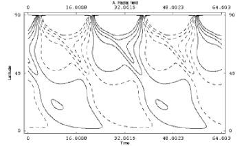
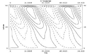
Figure 1: Butterfly diagrams for (A) the radial field at the surface ($r$$=$$R_{\odot}$) and (B) the toroidal magnetic field at the base of the solar convection zone ($r$$=$$0.7R_{\odot}$). The contours are equally spaced, with solid (dashed) lines for positive (negative) values. Time is in years and the latitude is in degrees. The maximum toroidal magnetic field at the base of the SCZ is located at latitudes between $75^{\circ}$ and $90^{\circ}$ with weak branches migrating toward the equator. With this result and based on magnetic flux tubes simulations, sunspots will appear mostly in regions close to the poles.

3.1 Deep Meridional Flow

If we allow the flow to go deeper ($r$$=$$0.61R_{\odot}$), a better distribution of the toroidal field lines is obtained, however, a polar branch also appears, in contrast to the observations and to the results Nandy & Choudhuri (2002) (Fig. 2).

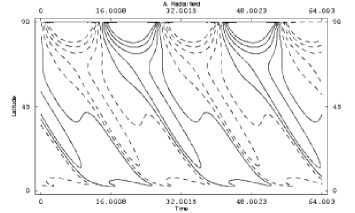
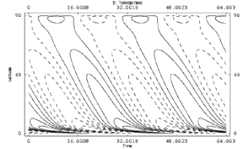
Figure 2: The same as in Fig. 1, but for a deeper meridional flow. If most of the magnetic field is dragged below the tachocline, only a small portion emerges to the surface by the action of the magnetic buoyancy force.

3.2 Exploring an ellipsoidal shape of the tachocline

Another way to test the deep meridional flow hypothesis is to change the form of the tachocline. In the helioseismic results of Charbonneau et al. (1999), they have reported a possible prolate shape of the tachocline. Though the full properties of the tachocline still remain unknown, we may here modify the shape of this layer by replacing the constant term $r_{c}$ in the equations above for a term that depends on $r$ and $\theta$ $r_{c}(r,\theta)$:

$$r_{c}(r,\theta)=\frac{r_{cx}r_{cy}}{\sqrt{r_{cx}^{2}\cos^{2}\theta+r_{cy}^{2}\sin^{2}\theta}},$$ (13)

where $r_{cx}$ and $r_{cy}$ are the semi-axis of an ellipse. If we first vary the term $r_{c}$ only in the differential rotation eqs. (6) and (10), in order to assure a substantial vertical shear, but maintaining it constant in eqs. (11) and (12), this configuration produces a prolate tachocline ($r_{cx}$$=$$0.67R_{\odot}$ and $r_{cy}$$=$$0.73R_{\odot}$) that generates weak polar branches (with magnetic fields of the order of $10^{4}$ G) and strong equatorward branches of toroidal field, in good agreement with the observations (see Fig. 3). In this case, the poloidal magnetic field, which is advected by meridional flows, goes deeper at the high latitudes within the more stable radiative layer. The toroidal field will diffuse more rapidly due to the longer values of the coefficient of diffusion in these latitudes. Advection then makes the rest of the process, draging this field to reach the tachocline and the convection zone, and arise to the surface. This scenario at which the flux goes deeper is more reliable because the mixture of elements occurs in a thinner layer within the radiative zone. If we now allow the $r_{c}$ term to vary according to eq. (13) also in the equations (11) and (12) and test this prolate configuration, we recover the results of the previous section (Fig. 2). A more detailed analysis will be presented elsewhere in a forthcoming paper.

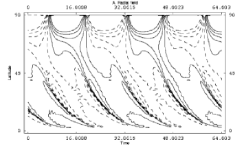
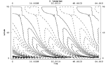
Figure 3: Butterfly diagrams for (A) the radial and (B) the toroidal magnetic fields assuming a prolate tachocline and a source term proportional to the toroidal magnetic field just above the tachocline.

4 Conclusions

We have recovered the Nandy & Choudhuri (2002) results and qualitatively reproduced the observed latitudinal distribution of the magnetic fields in the Sun assuming a different source formulation (Dikpati & Charbonneau, 1999). The most important results here found may be summarized as follows:

1. If the meridional flow is confined to the convective zone ($r$$>$$0.675R_{\odot}$), the sunspots are mainly concentrated near the poles.

2. If the flow is allowed to penetrate deeper down to $0.61R_{\odot}$, the model gives a better result since a branch of maximum toroidal field is produced at low latitudes in agreement with the observations. However, in this case, another branch also appears near the poles which is inconsistent with the observed butterfly diagrams.

3. When we incorporate a probably more realistic bipolytropic density profile in the tachocline and the radiative zone below the convective layer, the results above are maintained.

4. Finally, if we consider an ellipsoidal tachocline instead of a spherical one, we find that when a prolate shape is assumed and the magnetic field is stored mostly above the tachocline, then the resulting butterfly diagram is in good agrement with the observations.

5. The results above suggest that, although the models with a deep meridional flow are, in general, able to produce results which are in good agreement with the observations, the global behavior of the circulation and the physical mechanism behind it needs further revision in order to determine where the magnetic field is really amplified and stor ed (see Guerrero, de Gouveia Dal Pino & Munoz 2005, in preparation).

5 Acknowledgments

G.A.G. and E.M.G.D.P acknowledge financial support from the Brazilian Agencies CAPES and CNPq.

References

- A. R. Choudhuri (1995) M. Dikpati A. R. Choudhuri, M. Sch sler. The solar dynamo with meridional circulation. Astron. Astrophys, 303:L29, 1995.
- Charbonneau et al. (1999) P. Charbonneau, J. Christensen-Dalsgaard, R. Hening, R. M. Larsen, J. Schou, M. J. Thompson, & S. Tomczy. Helioseismic constrains on the structure of the solar tachocline. The Astrophysical Journal, 527:445–460, 1999.
- Chatterjee et al. (2004) P. Chatterjee, D. Nandy, & A. R. Choudhuri. Full-sphere simulations of a circulation-dominated solar dynamo: Exploring the parity issue. Astron. Astrophys, 427:1019–1030, 2004.
- Dikpati & Charbonneau (1999) M. Dikpati & P. Charbonneau. A babcock-leighton flux transport dynamo with solar-like differential rotation. The Astrophysical Journal, 518:508–520, 1999.
- Guerrero & Munoz (2004) G. Guerrero & J. D. Munoz. Kinematic solar dynamo models with deep meridional flow. MNRAS, 350:317–322, 2004.
- Kuker et al. (2001) M. Kuker, G. R diger, & M. Schultz. Circulation-dominated solar shell dynamo models with positive alpha-effect. Astron. Astrophys, 374:301–308, 2001.
- M. Dikpati (1994) A. R. Choudhuri M. Dikpati. The evolution of the sun’s poloidal field. Astron. Astrophys, 291:975–989, 1994.
- Nandy & Choudhuri (2001) D. Nandy & A. R. Choudhuri. Toward a mean field formulation of the babcock-leighton type solar dynamo. i. coefficient versus durney double-ring approach. The Astrophysical Journal, 551:576–585, 2001.
- Nandy & Choudhuri (2002) D. Nandy & A. R. Choudhuri. Explaining the latitudinal distribution of sunspots whit deep meridional flow. Science, 306:1671–1673, 2002.
- P. Caligari (1995) M Sch sler P. Caligari, F. Moreno-Insertis. Emerging flux tubes in the solar convection zone. 1: Asymmetry, tilt, and emergence latitude. The Astrophysical Journal, 441:886–902, 1995.
- P. Caligari (1998) M Sch sler P. Caligari, F. Moreno-Insertis. Emerging flux tubes in the solar convection zone. ii. the influence of initial conditions. The Astrophysical Journal, 502:481, 1998.
- Pinzón & Calvo-Mozo (2001) G. Pinzón & B. Calvo-Mozo. Low order p-modes in a bipolitropic model of the sun. astro-ph/0102429, 2001.
- S. D’Silva (1993) A. R. Choudhuri S. D’Silva. A theoretical model for tilts of bipolar magnetic regions. Astron. Astrophys, 272:621, 1993.
- Y. Fan (1993) E. E. DeLuca Y. Fan, G. H. Fisher. The origin of morphological asymmetries in bipolar active regions. The Astrophysical Journal, 405:390–401, 1993.