Magnetars

Abstract

Ultramagnetized neutron stars or magnetars are magnetically powered neutron stars. Their strong magnetic fields dominate the physical processes in their crusts and their surroundings. The past few years have seen several advances in our theoretical and observational understanding of these objects. In spite of a surfeit of observations, their spectra are still poorly understood. I will discuss the emission from strongly magnetized condensed matter surfaces of neutron stars, recent advances in our expectations of the surface composition of magnetars and a model for the non-thermal emission from these objects.

I INTRODUCTION

Simply put magnetars are neutron stars whose magnetic fields dominate their emission, evolution and manifestations. In the late 1970s and early 1980s, a fleet of sensitive detectors of high-energy radiation uncovered two new phenomena, the soft-gamma repeater and the anomalous x-ray pulsar. Strongly magnetized neutron stars provide the most compelling model for both types of object, and observations over the past few years indicate that these phenomena are two manifestations of the same type of object. Soft-gamma repeaters exhibit quiescent emission similar to that of anomalous x-ray pulsars (e.g 1994Natur.368..432R, ; 1994Natur.368..127M, ; 1996ApJ…463L..13H, ; 1999ApJ…510L.111H, ), and anomalous x-ray pulsars sometimes burst 2002Natur.419..142G ; 2003ApJ…588L..93K . What makes magnetars a hot topic of research is the rich variety of physical phenomena that strong magnetic fields exhibit.

This article will focus on the quiescent emission from these interesting objects rather than the bursts themselves (The reader may wish to refer to the seminal work of Thompson and Duncan Thom95 for details of the burst but may also want to look at Heyl and Hernquist Heyl03sgr for an alternative). Furthermore, the article will concentrate on recent results.

II MAGNETAR MANIFESTIONS

II.1 Soft-Gamma Repeaters

The first soft-gamma repeater was discovered on March 5, 1979 when gamma ray detectors on nine spacecraft across our solar system recorded an intense radiation spike 1979Natur.282..587M . The burst of gamma rays originated from near a supernova remnant known as N49 in the Large Magellanic Cloud. The tail of the gamma-ray burst exhibited an eight-second pulsation (in contrast with the classical gamma-ray bursts which show no periodicities). If one combined this eight-second period with the age of the supernova remnant and assumed that the object (presumably a neutron star) was born spinning much faster, one estimated a magnetic field on the object of $\sim 10^{15}$ G, much larger than any neutron star discovered up to that point.

This first SGR became known as SGR 0526-66. During 1979, two others were discovered: SGR 1806-20 (27 December 2004 event), SGR 1900+14 (28 August 1998 event) 1981Ap&SS..80….3M . In 1998 SGR 1627-41 became the fourth SGR to be discovered 1999ApJ…519L.139W .

Thompson & Duncan Thom95 ; Thom96 argued that the evolution of a ultrastrong magnetic field could explain both the outbursts and quiescent emission from soft-gamma repeaters, and the term “magnetar” was born. They argued earlier that if protoneutron star was born spinning sufficiently rapidly, a dynamo could dramatically amplify the standard pulsar magnetic field ($\sim 10^{12}$ G) that the protoneutron star was born with to $\sim 10^{15}$ G or more Thom93b .

II.2 Anomalous X-ray Pulsars

1E 2259+586 was the first anomalous x-ray pulsar to be discovered 1981Natur.293..202F . In the early nineties these objects began to form a unique class Mere95 ; Corb95 ; VanP95 ; Vasi97b . They were found to have much in common with the soft-gamma repeaters.

These objects typically have pulsed X-ray emission with steadily increasing periods of several seconds, X-ray luminosities of $\sim 10^{35}-10^{36}$ ergs s^-1, soft spectra, and no detected companions or accretion disks. Furthermore, they are typically observed through hydrogen column densities of $\sim 10^{22}$ cm^-2, indicating that they are not common.

Two of the five confirmed AXPs are located near the centres of supernova remnants 1E 2259+586 and 1E 1841-0451981Natur.293..202F ; Vasi97b as well as the AXP candidate AX J1845-0258 2000ApJ…542L..49V . The remaining objects are 4U 0142+61 1994ApJ…433L..25I , 1E 1048.1-5937 1986ApJ…305..814S , 1RXS J170849.0-400910 1997PASJ…49L..25S and possibly XTE J1810-197 2004ApJ…609L..21I .

The emission from the AXPs fits neatly within the magnetar model Thom96 . Heyl & Hernquist Heyl97kes argued that the thermal flux passing through an ultramagnetized, hydrogen or helium envelope is sufficient to account for the x-ray emission from these objects. Hey & Kulkarni Heyl98decay examined how magnetic field decay can augment the thermal energy budget. For fields less than about $10^{15}$ G magnetic field decay in a realistic model does not strongly affect the emission from young (less than 10,000 years) AXPs but can greatly increase their lifetime as observable x-ray sources.

Alternative models such as accretion have fallen by the wayside because even very low mass companions have not been discovered orbiting these neutron stars nor has the tell-tale optical emission from even a truncated accretion disk been detected.

II.3 Strongly Mangetized Radio Pulsars

Moreover, a number of radio pulsars have been discovered with inferred magnetic field strengths similar to those of magnetars and apparently exceeding the value $B_{{\hbox{\rm\scriptsize QED}}}\approx 4.4\times 10^{13}$ G 2000ApJ…541..367C ; 2002MNRAS.335..275M ; 2003ApJ…591L.135M It is not clear why these objects have magnetic fields comparable to the AXPs but do not exhibit AXP-like emission. The inferred magnetic field of AXP 1E2259+586 is actually smaller than PSR J1847-0130, an otherwise ordinary radio pulsar. The AXPs and SGRs exhibit much greater x-ray emission than their relatively inactive cousins. § III speculates further on the possible differences between these two types of objects.

III PHYSICS IN A STRONG MAGNETIC FIELD

Isolated neutron stars generally drawn on several sources of energy. For most observed neutron stars, the dominant source of energy is the rotation of the star.

$$E_{{\hbox{\rm\scriptsize rot}}}=\frac{1}{2}I\Omega^{2}\approx 2\times 10^{46}I_{45}\left(\frac{P}{1~{}{\hbox{\rm sec}}}\right)^{-2}~{}{\hbox{\rm erg}}$$ (1)

Magnetars are typically young, highly magnetized neutron stars. The magnetic energy,

$${\cal M}\,=\,{1\over{8\pi}}\,\int B^{2}\,dV\,\approx 2\times 10^{47}\,R_{6}^{3}\,B_{{\hbox{\rm\scriptsize NS,15}}}^{2}\,\,\,{\rm ergs},$$ (2)

exceeds the rotational energy by an order of magnitude. Nearly as large is the thermal energy of the star

$$U\,\sim\,10^{47}\,R_{6}^{2}\,M_{1.4}^{1/3}\,T_{8.5}^{2}\,\,\,\,{\rm ergs},$$ (3)

where $M_{1.4}$ and $T_{8.5}$ are the mass and core temperature of the star in units of $1.4M_{\odot}$ and $10^{8.5}$ K, respectively, and $R_{6}$ is the radius in units of 10 km and $B_{{\hbox{\rm NS}},15}$ is the surface magnetic field of the star in units of $10^{15}$ G. Much more weakly magnetized objects such as AXP 1E2259+586 act like magnetars as well. For this object $U\sim 100{\cal M}$.

It is unclear why some strongly magnetized neutron stars behave like “magnetars” rather than just happily spinning down and radiating as a radio pulsar. Not only do the soft-gamma repeaters and anomalous x-ray pulsars share a penchant for bursting (2003ApJ…588L..93K, , and Kaspi in these proceedings) that the pulsars lack they also generally have much stronger x-ray emission that radio pulsars – they are not only strongly magnetized but hot as well. As we have seen, for AXP 1E2259+586 the thermal energy exceeds a naive estimate of the magnetic energy by two orders of magnitude. It is quite natural to speculate that the heat flux travelling through the surface layers of the AXPs and SGRs may play an important role in their “magnetar” behaviour. A thermomagnetic interplay Blan83 between the strong magnetic field and the strong heat flux may help to power their bursts .

Gamma rays from by far the largest burst from a soft-gamma repeater arrived at Earth ten short days after the close of this meeting. The recent superbursts from SGR 1806-20 2005astro.ph..3030P ; 2005astro.ph..2577M ; 2005astro.ph..2541M brings many of these issues to the fore. Particularly the energy of this burst has been estimated to be $\approx 2\times 10^{46}$ erg 2005astro.ph..3030P , one hundred times that of the previous two superbursts from soft-gamma repeaters. It has been argued that this is a once in a century event 2005astro.ph..3030P . Given that detectors sensitive to such phenomena have only existed for 48 years (if one generously assumes that Sputnik and the Explorer satellites would have noticed such a burst), a once per century rate is rather conservative. To account for the number of observed SGRs, the soft-gamma repeaters must have a lifetime of several thousand years, so they would be expected to exhibit several dozens of such bursts. The budget of magnetic energy alone is insufficient to account for these bursts, so one is forced to conclude that either we are seeing the very end of the SGR phase for SGR 1806-20 or that the energy reservoir of SGR 1806-20 exceeds the magnetic energy stored in the dipole field.

Subsequent observations of SGR 1806-20 have reduced the estimate for its distance 2005astro.ph..3171M , but they still only obtain a lower limit to the distance. This result may reduce the energy budget for the event and ease the energy crisis. Further work is clearly needed.

Until the past year the observed quiescent emission from SGRs and AXPs was thought to be dominated by thermal emission. The following subsections discuss the various physical processes that determine the thermal emission from AXPs and SGRs (and possibly the non-thermal emission as well).

III.1 Vacuum Physics

For many purposes, vacuum polarization effects can be calculated using an effective Lagrangian for the electromagnetic field. Following the usual convention, we write

$${\cal L}\,=\,{\cal L}_{0}\,+\,{\cal L}_{1}\,+\,\cdots\,.$$ (4)

Here, ${\cal L}$ is the full Lagrangian density, ${\cal L}_{0}$ is the classical term, and ${\cal L}_{1}$ includes vacuum corrections to one-loop order. Higher order radiative corrections would be described by additional terms. The second-order term is smaller that ${\cal L}_{1}$ (Ditt85, ).

Because the Lagrangian is Lorentz invariant, both ${\cal L}_{0}$ and ${\cal L}_{1}$ can be expressed in terms of the Lorentz invariants of the electromagnetic field

$$I\equiv F_{\mu\nu}F^{\mu\nu}=2\left(|{\bf B}|^{2}\,-\,|{\bf E}|^{2}\right)$$ (5)

and

$$K\equiv\left[\epsilon^{\lambda\rho\mu\nu}F_{\lambda\rho}F_{\mu\nu}\right]^{2}=-4\left({\bf E}\cdot{\bf B}\right)^{2},$$ (6)

where $\epsilon^{\lambda\rho\mu\nu}$ is the completely antisymmetric Levi-Civita tensor. The effective Lagrangian of the electromagnetic field was derived by Heisenberg and Euler Heis36 and Weisskopf Weis36 using electron-hole theory. In rationalized Gaussian units, we can write ${\cal L}_{0}$ and ${\cal L}_{1}$ as

$${\cal L}_{0}\,=\,-{{1}\over 4}\,I\,,$$ (7)

$${\cal L}_{1}\, = \,{{\alpha}\over{2\pi}}\,\int_{0}^{\infty}\,{\rm e}^{-\chi}\,{{d\chi}\over{\chi^{3}}}\,\Biggr{[}$$

$$~{}~{}~{}i\,\chi^{2}\,{{\sqrt{-K}}\over 4}\,{{\cos(J_{+}\,\chi)+\cos(J_{-}\,\chi)}\over{\cos(J_{+}\,\chi)-\cos(J_{-}\,\chi)}}\,+$$

$$~{}~{}~{}\,B_{{\hbox{\rm\scriptsize QED}}}^{2}\,+\,I\,{{\chi^{2}}\over 6}\,\Biggr{]},$$

where

$$J_{\pm}\,\equiv\,{1\over{2B_{{\hbox{\rm\scriptsize QED}}}}}\,\left[-I\,\pm\,i\,\sqrt{-K}\right]^{1/2},$$ (9)

$\alpha\equiv e^{2}/\hbar c$ is the fine structure constant, $B_{{\hbox{\rm\scriptsize QED}}}\equiv m^{2}c^{3}/e\hbar\approx 4.4\times 10^{13}$ G, and a similar quantity can be defined for the electric field, $E_{{\hbox{\rm\scriptsize QED}}}\equiv m^{2}c^{3}/e\hbar\approx 2.2\times 10^{15}$ V/cm. The above expressions for ${\cal L}_{0}$ and ${\cal L}_{1}$ are identical to the corresponding terms in eq. (45a) of Heisenberg & Euler Heis36 .

The above integral cannot be evaluated explicitly, in general. Heyl & Hernquist Heyl97hesplit have derived an analytic expression for ${\cal L}_{1}$ as a power series in $K$:

$${\cal L}_{1}\,=\,{\cal L}_{1}(I,0)\,+\,K\,{{\partial{\cal L}_{1}}\over{\partial K}}\Bigg{|}_{K=0}\,+\,\cdots\,,$$ (10)

where the first term in this series is

$${\cal L}_{1}(I,0) = {\alpha\over{4\pi}}\,I\,X_{0}\left({1\over\xi}\right)$$

$$= {\alpha\over{4\pi}}\int_{0}^{\infty}{\rm e}^{-u/\xi}{{du}\over{u^{3}}}\left(-u\coth u+1+{{u^{2}}\over 3}\right),$$

and

$$\xi\,=\,{1\over B_{{\hbox{\rm\scriptsize QED}}}}\,\sqrt{{I\over 2}}=\frac{B}{B_{{\hbox{\rm\scriptsize QED}}}},\,$$ (13)

where the final equality holds if the electric field can be neglected.

The function $X_{0}$ can be evaluated analytically (as can the higher order terms in the expansion for ${\cal L}_{1}$) with the result Heyl97hesplit

$$X_{0}(x)\, = \,4\int_{0}^{x/2-1}\,\ln(\Gamma(v+1))\,dv\,-\,{1\over 3}\,\ln x\,+\,{\cal C}\,$$

$$~{}~{}~{}-\,\left[1\,+\,\ln\left({{4\pi}\over x}\right)\right]\,x\,$$

$$~{}~{}~{}+\,\left[{3\over 4}\,+\,{1\over 2}\,\ln\left({2\over x}\right)\right]\,x^{2}\,,$$

where

$${\cal C}\,=\,2\ln 4\pi\,-\,4\ln A\,-{5\over 3}\ln 2\,=\,2.911785285,$$ (15)

and the constant $\ln A$ is related to the first derivative of the Riemann zeta function, $\zeta^{(1)}(x)$, by

$$\ln A\,=\,{1\over{12}}\,-\,\zeta^{(1)}(-1)\,=\,0.248754477\,.$$ (16)

The integral of $\ln\Gamma(x)$ can be expressed in terms of special functions (eqs. 18, 19 in Heyl97hesplit ). (See also Dittrich et al. 1979; Ivanov 1992, but note the cautionary remark in Heyl97hesplit .)

The expression above for $X_{0}(x)$ can be expanded in either a Taylor series in the weak field limit, $\xi\ll 1$, or an asymptotic series in the strong field limit $\xi\gg 1$, as can the higher order terms in equation (10), to give series expansions for ${\cal L}_{1}$ as a function of either $I$ and $K$, or equivalently $B$ and $E$. In particular, to lowest order in the weak field limit ($\xi\ll 1$)

$${\cal L}_{1}\,=\,{{\alpha}\over{90\pi}}\,{1\over{B_{{\hbox{\rm\scriptsize QED}}}^{2}}}\left[(B^{2}\,-\,E^{2})^{2}\,+\,7({\bf E}\cdot{\bf B})^{2}\right]\,+\,\cdots$$ (17)

In the limit of an ultrastrong magnetic field, $B\gg B_{{\hbox{\rm\scriptsize QED}}}$, but for a weak electric field, $E\ll E_{{\hbox{\rm\scriptsize QED}}}$, ${\cal L}_{1}$ can be written

$${\cal L}_{1}\,=\,{{\alpha}\over{6\pi}}\,B^{2}\,\left[\ln\left({B\over{B_{{\hbox{\rm\scriptsize QED}}}}}\right)\,-\,12\ln A\,+\,\ln 2\right]\,+\,\cdots\,$$ (18)

(see e.g. eq. 29 in Heyl97hesplit for the higher order terms). We note that equations (17) and (18) agree, respectively, with the corresponding terms in eqs. (43) and (44) of Heis36 . The analysis of Heyl97hesplit generalizes the expressions of Heisenberg & Euler to arbitrary order.

Also, note that while our expression for ${\cal L}_{0}$ is identical to eq. (4-120) of Itzykson & Zuber Itzy80 , equation (17) differs from their eq. (4-125) by a factor of $1/4\pi$, as a consequence of a difference in the system of units employed. Our expressions for ${\cal L}_{0}$ and ${\cal L}_{1}$ both differ from those in Berestetskii et al. Bere82 by an overall factor of $1/4\pi$ (their eqs. 129.2 and 129.21); however, the dynamics of the fields are invariant with respect to rescalings of the Lagrangian.

We emphasize that the expression for the Lagrangian in the weak-field limit, equation (17), cannot be applied to magnetar fields which are thought to have $B_{{\hbox{\rm\scriptsize NS}}}\gg B_{{\hbox{\rm\scriptsize QED}}}$. The use of the weak-field expressions to calculate, e.g. the index of refraction of the vacuum near the surface of a magnetar will result in estimates that are incorrect by more than an order of magnitude at the relevant field strengths. In this limit, the Lagrangian should instead be approximated by e.g. equation (18), which is an asymptotic series for ${\cal L}_{1}$ valid for $B\gg B_{{\hbox{\rm\scriptsize QED}}}$ and $E\ll E_{{\hbox{\rm\scriptsize QED}}}$.

After integrating out the effects of the virtual electron-positron pairs, one is left with an effective Lagrangian and many electromagnetic phenomena can be treated by simply treating the vacuum itself as a medium endowed whose properties are described by the Lagrangian. This approximation is valid for photon energies much less than $m_{e}c^{2}$. For higher energy photons the assumption of a homogeneous field implicit in the above construction of the effective Lagrangian breaks down and one must resort to other methods (for example Schw51, ).

III.2 Atomic Physics

The atomic physics of materials on the surfaces of magnetars is dominated by the magnetic field rather that the atomic nucleus. A useful figure of merit is the ratio of the cyclotron energy of an electron to the binding electron of an electron to a nucleus of atomic number $Z$

$$\frac{E_{{\hbox{\rm\scriptsize cyclo}}}}{E_{{\hbox{\rm\scriptsize Rydberg}}}} = \frac{m_{e}c^{2}B/B_{{\hbox{\rm\scriptsize QED}}}}{Z^{2}/2\alpha^{2}m_{e}c^{2}}=\frac{2B}{\alpha^{2}Z^{2}B_{{\hbox{\rm\scriptsize QED}}}}$$ (19)

$$= \frac{B}{1.1Z^{2}\times 10^{9}~{}{\hbox{\rm G}}}$$ (20)

where $B_{{\hbox{\rm\scriptsize QED}}}$ is defined in §III.1. We see for magnetars this ratio is large for $Z$ up to one hundred or more. The atomic physics is in this regime has been probed extensively for hydrogen and helium (for example Rude94, ; Heyl98atom, ) but approximately for larger atoms such as iron 1991MNRAS.253..107M .

What remains uncertain is how these atoms interact and what are the properties of strongly magnetized material in the bulk at low pressure. Is it a solid, liquid or gas? Is it metallic? These questions are crucial to understand the details of the thermal emission from neutron stars. For further details on the physics of atoms and molecules in strong magnetic fields the reader is urged to consult the excellent review of Lai 2001RvMP…73..629L .

III.3 Thermal Physics

Through much of the envelope of a magnetar the electron gas is effectively one-dimensional because only the first Landau level is typically filled Heyl97analns ; Heyl98numens . This restriction dramatically affects the thermodynamic properties of the material and allows approximate yet reasonably accurate analytic treatment of the thermal conduction through the envelope of a magnetar Heyl97analns .

The key parameters are the chemical potential of the electrons, the temperature and the strength of the magnetic field. It is helpful to define the dimensionless quantities,

$$\zeta=\frac{\mu_{e}}{m_{e}c^{2}},\,x^{2}=\zeta^{2}-1,\,\tau=\frac{kT}{m_{e}c^{2}}$$ (21)

in addition to $\xi=B/B_{{\hbox{\rm\scriptsize QED}}}$ from § III.1. The number density of electrons in the degenerate limit ($\tau\ll\ \zeta-1$) is given by

$$n_{e,0}=\frac{1}{3\pi^{2}{\lambda\!\!\!\!\hskip 0.56905pt^{-}}^{3}}x^{3}$$ (22)

for a weakly magnetized gas ($x\gg\ 2\xi$) and

$$n_{e,{{\hbox{\rm\scriptsize magnetar}}}}=\frac{\xi}{2\pi^{2}{\lambda\!\!\!\!\hskip 0.56905pt^{-}}^{3}}x$$ (23)

for a strongly magnetized gas. The symbol ${\lambda\!\!\!\!\hskip 0.56905pt^{-}}$ denotes the Compton wavelength of the electron, $\hbar/(m_{e}c)$.

The pressure of the magnetized gas also differs from the unmagnetized case. The number density of electrons in the degenerate limit ($\tau\ll\ \zeta-1$) is given by

$$P_{e,0}=\frac{1}{8\pi^{2}}\frac{m_{e}c^{2}}{{\lambda\!\!\!\!\hskip 0.56905pt^{-}}^{3}}\left[x\zeta\left(\frac{2}{3}\zeta^{2}-\frac{5}{3}\right)+\ln(x+\zeta)\right]$$ (24)

for a weakly magnetized gas ($x\gg\ 2\xi$) and

$$P_{e,{{\hbox{\rm\scriptsize magnetar}}}}=\frac{\xi}{4\pi^{2}}\frac{m_{e}c^{2}}{{\lambda\!\!\!\!\hskip 0.56905pt^{-}}^{3}}\left[x\zeta-\ln(x+\zeta)\right]$$ (25)

for a strongly magnetized gas. Although the magnetic field changes the pressure dramatically, the electric pressure remains isotropic due to the changing mangetization as the electrons are compressed Hern85 .

An important comparison is at what density do the electron become degenerate in the two cases. Magnetar envelopes are generally cool, $\tau\ll 1$ so $\zeta-1\approx x^{2}/2\approx\tau$ at the onset of degeneracy. The ratio of the densities of the gas at the onset of degeneracy in unmagnetized and the ultramagnetized case is given by

$$\frac{n_{e,{{\hbox{\rm\scriptsize magnetar}}}}}{n_{e,0}}=\frac{3}{2}\frac{\xi}{x^{2}}=\frac{3}{4}\frac{\xi}{\tau}\gg 1.$$ (26)

The ratio of the pressures at the onset of degeneracy is given by a similar factor. For a magnetar, $\xi\sim 10-100$ and $\tau\sim 10^{-1}$, yielding a factor of 100$-$1000 increase in the density, column density and pressure at the onset of degeneracy. Magnetar envelopes only become degenerate densities larger than

$$\rho_{{\hbox{\rm\scriptsize ND/D}}} = 3.92\times 10^{5}{\hbox{\rm g cm}}^{-3}\xi(\ln b_{{\hbox{\rm\scriptsize Typical}}})^{1/7}$$ (27)

$$~{}~{}~{}\times A_{56}^{6/7}Z_{26}^{-5/7}T_{{\hbox{\rm\scriptsize eff,6}}}^{4/7}g_{s,14}^{-1/7}.$$

where $b_{{\hbox{\rm\scriptsize Typical}}}$ is a typical value of $\xi/\tau$ in the envelope, $b_{{\hbox{\rm\scriptsize Typical}}}\approx 6\times 10^{3}\xi$. The unmagnetized envelope become degenerate at densities $\sim 10^{2}-10^{4}$ g cm^-3 Hern84b .

IV THERMAL EMISSION FROM MAGNETARS

The thermal emission from magnetars is powered by a combination of the residual heat from the supernova explosion (Eq. 3)and possibly the magnetic field (Eq. 2). The accretion alternative predicts more optical emission than is observed from these objects (but see 2003ApJ…599..450E, , for an alternative point of view). If the thermal energy originates from within the star, the energy must first travel through the insulating envelope of the neutron star. The conductivity of this layer throttles the heat flow and determines the total thermal emission from these objects.

In the non-degenerate regime, the conductivity is nearly constant and determined by the outgoing heat flux both for magnetars and weakly magnetized neutron stars Hern84b ; Heyl97analns . The photons in the extraordinary polarization mode dominate the heat conduction, and the conductivity itself is strongly dependent on the magnetic field. In the degenerate regime the conductivity increases dramatically. Along the field lines, the strong magnetic field strengthens the heat conduction, while across the field lines, the field inhibits it. For a fixed internal temperature of the star, the emerging flux is approximately proportional to $Z^{-0.7}B^{0.4}\cos^{2}\psi$ where $\psi$ is the angle between the local magnetic field ($B$) and the normal and $Z$ is the atomic number of the nuclei that comprise the envelope Heyl97analns ; Heyl97kes . Potekhin et al. 2003ApJ…594..404P examined the dependence of the cooling of neutron stars (including the superfluidity of their interiors) on the presence of a light-element envelope in further detail, verifying the earlier conclusions.

IV.1 Magnetized Atmospheres

The study of mangetized neutron stars is simplified by the fact that neutron stars atmospheres are exceedingly thin. Unfortunately, this is an inadequate consolation for the complications that the strong magnetic fields introduce.

• As discussed in § III.2 the binding energies of even light species such as hydrogen and helium may exceed several hundred electron volts in the magnetar fields, so magnetar atmospheres are probably only partially ionized (see Figs. 1 and 2 of 2004ApJ…600..317P, ). The light element atmospheres of more weakly magnetized stars are typically fully ionized, but even in weak fields heavier species such as carbon, oxygen and others will not be fully ionized. The presence of bound species affects not only the opacity of the plasma but also its equation of state and electromagnetic polarization.

• The opacities for the two polarization modes differs by several orders of magnitude, so the polarized radiative transfer must be calculated.

• Vacuum polarization (§ III.1) complicates the behaviour of the propagation modes of the plasma itself. As radiation propagates through the vacuum resonance where the vacuum and plasma contribute equally to the index of refraction, the mode that below the resonance had the higher opacity now has the lower opacity and vice versa. This effect complicates the radiative transfer for for radiation slightly above the peak of the thermal distribution 2002ApJ…566..373L ; 2003ApJ…583..402O .

• The opacites depend strongly on the direction of that the radiation propagates relative to the magnetic field. Where the field is normal to the surface only the altitude is important (like in unmagnetized transfer) but the distribution must be sampled more finely to handle the sensitive angular dependence. Where the field is makes an angle with respect to the normal (the general case), the intensity must be calculated both in altitude and azimuth.

The recent work of Potekhin et al.2004ApJ…612.1034P may be considered an example of the state of the art in magnetized atmospheres. Fig. 1 depicts the results for calculations that fully include the effects of partial ionization and vacuum polarization as well as spectrum using less realistic assumptions. The shape of the spectrum changes dramatically as the calculations become more sophisticated. Even from these comprehensive simulations, several important effects are absent. First, the magnetic field is assumed to pointing in the normal direction. Relaxing this constraint makes the calculations more onerous but similar in principle and is required to simulate the emission from the entire surface of the neutron star. Second, the magnetic field is still two orders of magnitude less than that of magnetars. As the magnetic field increases the difference in the opacities between the two modes increases and also the material in the outer layers may undergo a phase transition 2004astro.ph..6001V . Finally the surface layers may not consist of hydrogen but rather helium or heavier elements (see § IV.4).

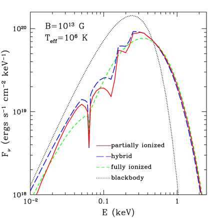
Figure 1: The total emergent spectrum from a strongly magnetized neutron star atmosphere from the calculations of Potekhin et al. 2004ApJ…612.1034P . A blackbody spectrum is compared with several atmospheric calculations of increasing realism. The fully ionized model assumes that neutral species are absent. The hybrid model includes partial ionization to calculate the equation of state and the opacity but assumes that polarization modes are those of a fully ionized plasma. The partially ionized model includes the effects of partial ionization on the opacity, equation of state and polarization. All of the models include vacuum polarization

A tantalizing alternative is that magnetar atmospheres aren’t atmospheres at all, but rather the surface of a magnetar is condensed. The condensation temperature may be as high as $10^{6}$ K for iron in fields stronger than $10^{13}$ G and even for hydrogen in fields of a few $\times 10^{14}$ G. In this situation detailed balances allows the emergent spectrum from the star to be determined by understanding how light reflects off of it. Van Adelsberg et al. 2004astro.ph..6001V calculate emergent thermal spectra from the condensed surface of a magnetar. If the surface is smooth, the spectrum deviates from a blackbody by at most a factor of two and exhibits only mild absorption features that correspond to the ion cyclotron resosonace and the plasma frequency within the surface. The emission for rough surfaces resembles that of a blackbody more closely.

Figure 2: The total emergent spectrum from a strongly magnetized condensed neutron star atmosphere from the calculations of van Adelsberg et al. 2004astro.ph..6001V .

IV.2 Magnetospheric Propagation

Regardless of the detailed composition of the atmosphere of magnetars, the vast difference between the opacities in the two polarization modes nearly ensures that the radiation will emerge from the atmosphere highly polarized perpendicular to the direction of the local magnetic field. Pavlov and Zavlin 2000ApJ…529.1011P argued that because the direction of the magnetic field varies across the surface of the neutron stars, the net polarization from the entire visible surface is greatly diminished. This argument neglects that the region surrounding the magnetar is optically active. Specifically at the x-ray energies, the the intense magnetic field decouples the propagation modes in the magnetosphere through vacuum polarization (§ III.1). Heyl and Shaviv Heyl01qed argued that polarized radiation propagates adiabatically through the magnetosphere. The adiabatic condition holds within the polarization-limiting radius (see Chen79, , for the plasma analogue),

$$r_{{\hbox{\rm\scriptsize pl}}} \equiv \left(\frac{\alpha}{45}\frac{\nu}{c}\right)^{1/5}\left(\frac{\mu}{B_{{\hbox{\rm\scriptsize QED}}}}\sin\beta\right)^{2/5}$$

$$\approx 1.2\times 10^{7}\left(\frac{\mu\sin\beta}{10^{30}~{}{\hbox{\rm G cm}}^{3}}\right)^{2/5}\left(\frac{\nu}{10^{17}~{}{\hbox{\rm Hz}}}\right)^{1/5}{\hbox{\rm cm}},$$

where $r$ is the distance from the center of the star, $\mu$ is the magnetic dipole moment of the neutron star, and $\beta$ is the angle between the dipole axis and the line of sight. The observed polarization reflects not the direction of the magnetic field at the surface of the star but at the polarization-limiting radius; consequently, if this radius is much larger than the radius of the star, the polarized radiation from disparate regions of the stellar surfaces adds conherently an a large net polarization results.

Fig. 3 depicts the polarized spectrum summed over the entire surface of the neutron star. The local emergent radiation spectrum is determined from an atmospheric model that assumes that the plasma is fully ionized hydrogen and neglects vacuum polarization within the atmosphere. The bold curves trace the results from a calculation that includes vacuum polarization within the magnetosphere and the light curves neglect vacuum polarization. If vacuum polarization within the magnetosphere is included the radiation is more than 99% polarized near the peak of the spectrum. Without it the total emission is more modestly polarized by about 10%.

Figure 3: The total emergent flux from the visible surface of the star. The magnetic pole makes an angle of 60^∘ with the line of sight. The radius of the star is 12 km and its mass is 1.4 M_⊙. The effective temperature at the magnetic pole is $10^{6.5}$ K. The calculation is for $\mu=10^{32}$ G cm³, corresponding to a surface field of $\sim 10^{14}$ G respectively. The solid curve traces the total flux. The short dashed curve traces the flux polarized perpendicular to the projection of the magnetic moment in the plane of the sky. The long-dashed curve traces the flux polarized parallel to the projected magnetic moment. The heavy curves trace the results including vacuum polarization and the light curves neglect it.

In the X-ray regime, the radiation from the entire surface of the neutron star is highly polarized for surface magnetic fields greater than $10^{12}$ G or so. At lower photon energies, especially in the optical and infrared, the observed polarization is a sensitive probe of the magnetic field and plasma density within the magnetosphere as well as the radius of the neutron star Shan04 . Polarimetry of magnetars and neutron stars in general will provide a unique new probe of their environments and interiors.

IV.3 Magnetic Field Decay

Thompson and Duncan Thom96 argued that the decay of the strong magnetic field of a magnetar could account for the quiescent emission from the surface and examine the gradual evolution of the magnetic field of the star. Goldreich and Reisenegger Gold92 examine several modes of magnetic field decay: Ohmic diffusion, Hall drift and ambipolar diffusion. These processes have the following timescales:

$$t_{{\hbox{\rm\scriptsize Ohmic}}} \sim 2\times 10^{11}\frac{L_{5}^{2}}{T_{8}^{2}}\left(\frac{\rho}{\rho_{{\hbox{\rm\scriptsize nuc}}}}\right)^{3}{\hbox{\rm~{}yr}}$$ (29)

$$t^{{\hbox{\rm\scriptsize s}}}_{{\hbox{\rm\scriptsize ambip}}} \sim 3\times 10^{9}\frac{L_{5}^{2}T_{8}^{2}}{B_{12}^{2}}{\hbox{\rm~{}yr}}$$ (30)

$$t^{{\hbox{\rm\scriptsize irr}}}_{{\hbox{\rm\scriptsize ambip}}} \sim \frac{5\times 10^{15}}{T_{8}^{6}B_{12}^{2}}{\hbox{\rm~{}yr}}+t^{{\hbox{\rm\scriptsize s}}}_{{\hbox{\rm\scriptsize ambip}}}$$ (31)

$$t_{{\hbox{\rm\scriptsize Hall}}} \sim 5\times 10^{8}\frac{L_{5}^{2}T_{8}^{2}}{B_{12}}\left(\frac{\rho}{\rho_{{\hbox{\rm\scriptsize nuc}}}}\right){\hbox{\rm~{}yr}}$$ (32)

where $L_{5}$ is a characteristic length scale of the flux loops through the outer core in units of $10^{5}$ cm, $T_{8}$ is the core temperature in units of $10^{8}$ K and $B_{12}$ is the field strength in units of $10^{12}$ G. Ohmic decay dominates in weakly magnetized neutron stars ($B\lesssim 10^{11}$ G), fields of intermediate strength decay ($B\sim 10^{12}-10^{13}$ G) via Hall drift, and intense fields ($B\gtrsim 10^{14}$ G) are mostly strongly affected by ambipolar diffusion. Thompson and Duncan Thom96 examined the possibility of obtaining an equilibrium between neutrino cooling and heating through magnetic field decay for $B\sim 10^{15}$ G and $T\sim 10^{8}$ K.

In the case of a magnetar older than a few hundred years, ambipolar diffusion dominates the other porcesses at least in the core of the neutron star. Ambipolar diffusion involves motion of the charged species (electrons, protons and possibly muons) relative the the neutrons. In the motion of the change species results a change in the density of these particles (if the flow is irrotational), the chemical equilibrium must be reestablished through weak interactions. Otherwise the flow is solenoidal and weak reactions are not required.

Using the results of Goldreich and Reisenegger Gold92 , Heyl and Kulkarni Heyl98decay examined how magnetic field decay would affect the thermal emission from the surface of a magnetar and its cooling, including a realistic treatment of the strongly magnetized envelope of the neutron star. Fig. 4 shows the results of their analysis. If the magnetic field is sufficiently strong ($B\sim 10^{16}$ G) field decay has a dramatic effect on the emission from young magnetars, less than ten thousand years old. Even without field decay the magnetic field dramatically increases the heat flux through the surface of the neutron star. For intermediate fields ($B\sim 10^{15}$ G) field decay does not strongly affect the emission of the young magnetars, but for fields similar to and stronger than $10^{15}$ G field decay increases the lifetime of hot magnetars by a factor of several. This dramatically increases the number of hot magnetars that you would expect to see in the Galaxy and possibly the evolution of soft-gamma repeaters and anomalous x-ray pulsars.

Figure 4: The left panel depicts the evolution of the effective temperature (left) and magnetic field (right) magnetic field decays through the solenoidal mode. The right panel depicts the results for decay through the irrotational mode. The bold solid, dotted and dashed lines give the results for $B_{i}=10^{14},10^{15}$ and $10^{16}$ G respectively. The light lines give the results without any field decay, and the long-short-dashed line gives the cooling evolution for an unmagnetized neutron star.

IV.4 Diffusion

A crucial input for our understadning of the emission from thes surface of neutron stars is the composition of their outer layers. As discussed in § III.3 and § IV.1 the presence of light elements in these layers can have a dramaticially effect on the total thermal emissiokn from the star as well as its spectrum. The strong gravitiational acceleration at the surface of the neutron star ($g\sim 10^{14}$ cm s^-2) ensures that the lighter elements will float to the top of the atmosphere; consequently, one would expect the emergent spectrum and flux to be determined by the lightest elements present in the outermost fluid layers of the star. If any material fell back onto the neutron star during or after the supernova, it spallates as it hits the surface, resulting in hydrogen and helium nuclei.

The thickness of a pure hydrogen layer is limited the stabilty of protons against decaying into neutrons. If the chemical potential of the electrons exceeds mass difference between a proton and a neutron ($\zeta\approx 2.53,x\approx 2.33$) it becomes energetically favourable for protons to combine with electrons and form neutrons. These neutrons will quickly bind to protons, forming deuterons and ultimately helium nuclei.

According to equations 22 and 23, this occurs at a density of about $1.2\times 10^{7}{\hbox{\rm g cm}}^{-3}$ for a weakly magnetized gas and about $3.4\xi\times 10^{6}{\hbox{\rm g cm}}^{-3}$ for a strongly magnetized gas in which $\xi\gg 1$.

The thickness of the hydrogen layer that can be supported on a magnetar increases with the strength of the magnetic field. The thickness of a helium layer is assumed to be limited by the shell flash instability that results in Type-I X-ray bursts on neutron stars. This criterion yields a maximum column density of a helium layer of approximately $10^{8-9}$ g cm^-2 (e.g. Nara03typei, ). It is unclear whether the strong magnetic field affects nuclear burning of helium, but it does affect hydrogen burning Heyl96fus . If a neutron star accretes more than about $10^{22}$ g of material after its birth, one would expect find moving from the outside inward hydrogen, helium and then carbon or other heavier elements.

These results neglect the fact that although the layers are stabily stratified, a thermally excited tail of protons will penetrate the layer of helium and possibly be captured onto the carbon and other nuclei lying below. Chang, Arras and Bildsten 2004astro.ph.10403C examined this problem in detail. As protons diffuse through the helium layer, their density drops as a power law in the non-degenerate regime and exponetially in the degenerate regime. In a magnetar the electrons become degenerate at a much higher column density than in a neutron star with a smaller magnetic field (Eq. 27). Although diffusive nuclear burning is not terribly important over the timescale of a few thousand years for weakly magnetized neutron stars, in magnetars a thin atmospheric hydrogen layer is consumed as protons diffuse through a maximally thick helium layer in only a few years.

The efficiency of diffusive nuclear burning on a magnetar indicates that the atmospheres and enevlopes of magnetars likely consist of helium or heavier elements rather than hydrogen. Because ionized hydrogen atmospheres has generally be the focus of research into magnetar atmosphere (see § IV.1) clearly more work is needed.

V NON-THERMAL EMISSION FROM MAGNETARS

Until the past year the quiescent emission from magnetars was thought to be mostly due to thermal emission from the surface of the star. Their soft x-ray spectra are notoriously well described by blackbody models (possibly with a power-law component at high energies) (for example Pern00axp, ). However, recent results from INTEGRAL indicate that the thermal emission is just the tip of the iceberg (2004astro.ph.11695M, ; 2004ATel..293….1D, ; 2004astro.ph.11696M, , and Hurley in these proceedings). The optical emission from AXPs is also clearly non-thermal (or at least not from the surface) 2004astro.ph..4144O .

Thompson and Beloborodov 2004astro.ph..8538T present two models to account for the non-thermal hard x-ray emission from the AXP 1E 1841-045. The first involves the heating of a surface layer of the neutron star to $kT\sim 100$ keV by currents driven in the magnetosphere by the twisting of the magnetic field in the crust. The second model focusses on a region far from the star (at ten stellar radii) where the electron cyclotron resonance is approximately 1 keV. The thermal flux from the surface exerts a force on the current-carrying electrons in this region and a large electric field develops. A positron injected into this region quickly accelerates to energies where it can upscatter keV photons above the threshold for pair creation. The pairs emit synchrotron radiation consistent with the observed spectrum.

Heyl and Hernquist Heyl05sgr present an alternative picture that can account for both the optical and hard x-ray non-thermal emission. § III.1 outlines the dynamics of the electromagnetic field including radiative corrections. A key result is that the effective Lagrangian of QED makes electrodynamics non-linear. Specifically simple electromagnetic waves travelling through a strong magnetic field develop regions when the electric and magnetic field are discontinuous – shocks Heyl98shocks . These shocks also form as fast waves travel through an ultramagnetized, ultrarelativistic plasma Heyl98mhd .

As a fast wave propagates away from the surface of the neutron star and forms a shock, the energy release in the shock powers the formation of electron-positron pairs at rest in the frame of the shock. These pairs emit synchrotron photons that produce more pairs. This pair cascade stops because the total optical depth for pair creation strongly decreasing with the energy of the photons. The final generation of pairs has a typical Lorentz factor of $\gamma=0.05\xi^{-1}$ with $\xi\ll 1$ far from the surface of the star. These pairs emit synchrotron photons with an energy ranging from

$$E_{{\hbox{\rm\scriptsize break}}}=\gamma^{2}\hbar\omega_{B}\approx 2.5\times 10^{-3}\xi^{-1}mc^{2}.$$ (33)

down to $E_{0}=\xi mc^{2}$. At each radius the pairs cool in a fixed magnetic field, yielding a spectrum $dE\propto E_{\gamma}^{-1/2}dE_{\gamma}$ between the values of $E_{0}$ and $E_{{\hbox{\rm\scriptsize break}}}$ at the innermost edge of the pair production region. At energies greater than $E_{{\hbox{\rm\scriptsize break}}}$ or less than $E_{0}$ the emission comes from pairs produced further from the star. Simulations of the fast-mode breakdown in a dipole geometry Heyl05sgr indicate that the fast mode delivers equal amounts of energy in equal ranges of mangetic field, yielding the complete spectrum

$$\frac{dE}{dE_{\gamma}}\propto\left\{\begin{array}[]{lc}E_{\gamma},&E_{{\hbox{\rm\scriptsize min}}}<E_{\gamma}<E_{0}\\ E_{\gamma}^{-1/2},&E_{0}<E_{\gamma}<E_{{\hbox{\rm\scriptsize break}}}\\ E_{\gamma}^{-2},&E_{{\hbox{\rm\scriptsize break}}}<E_{\gamma}<E_{{\hbox{\rm\scriptsize max}}}\end{array}\right.$$ (34)

The model has two free parameters: the total energy delivered by the fast mode $E_{{\hbox{\rm\scriptsize total}}}$ and the strength of the magnetic field at the inner edge of the pair-production region that determines the location of both break points.

Fig. 5 compares the spectrum of non-thermal radiation produce by fast-mode breakdown with the non-thermal radiation observed from the AXPs 4U 0142+61 and 1E 1841-045 and the SGR 1806-20. The model accounts for the observed spectral slope both in the optical and in the hard x-ray. If we assume that all of the objects have similar intrinsic optical emission to the nearby AXP 4U 0142+61, we predict that the non-thermal emission should peak around 100 MeV as traced by the curves denoted as the “Optical Model” for AXP 4U 0142+61 and as the “Unified Model” for the other two objects. On the other hand if 1E 1841-045 and the SGR 1806-20 do not exhibit a similar optical excess to 4U 0142+61, the non-thermal emission should extend to at least 1 MeV as depicted by the “Minimal Model” curves.

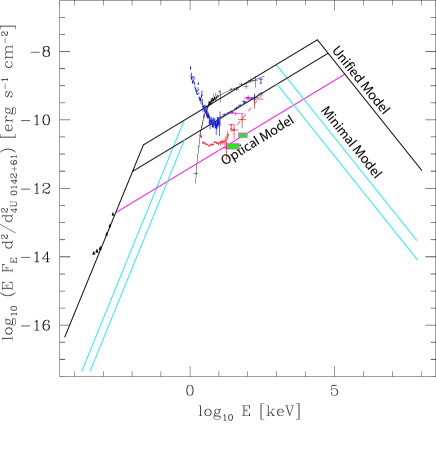
Figure 5: The spectrum produced by fast-mode breakdown is superimposed over the observed thermal and non-thermal emission from several AXPs and SGRs for models that fit either the optical or INTEGRAL data solely and one that fits both sets of data. The unabsorbed optical data are from Hulleman et al. 2000Natur.408..689H via Özel 2004astro.ph..4144O for AXP 4U 0142+61. The uppermost black symbols are the hard X-ray band are from Molkov et al. 2004astro.ph.11696M for SGR 1806-20. Mereghetti et al. 2004astro.ph.11695M obtained similar results for the SGR. The middle sets of points in the hard X-ray data (blue is total flux and red is pulsed flux) are from Kuiper et al.2004ApJ…613.1173K for AXP 1E 1841-045. The green squares plot the INTEGRAL data reported by den Hartog et al. 2004ATel..293….1D for AXP 4U 0142+61. We normalised the den Hartog et al.2004ATel..293….1D results using the observations of the Crab by Jung 1989ApJ…338..972J . We scaled the emission from the three sources by assuming that they all lie at the distance of AXP 4U 0142+61. We used 3 kpc for AXP 4U 0142+61 2000Natur.408..689H , 7.5 kpc for AXP 1E 1841-045 1992AJ….104.2189S and 15 kpc for SGR 1806-20 2004astro.ph.11696M .

EGRET determined upper limits for the gamma-ray flux from the direction of these objects. Tab. 1 gives these upper limits and the predictions of the fast-mode breakdown model. The optical model and the unified model predict approximately similar EGRET fluxes for 4U 0142+61. The minimal model based solely on the INTEGRAL data exhibits a flux above 100 MeV about two hundred times smaller than the unified model. Because the optical model cannot explain the observed INTEGRAL data for 1E 1841-045 and SGR 1806-20, it is omitted. Similarly, the minimal model cannot explain the optical data for 4U 0142+61. We see that for 1E 1841-045 and SGR 1806-20 the predictions for the minimal model lie comfortably below the EGRET upper limits. In the context of the fast-mode breakdown model, this means that the optical emission for 1E 1841-045 and SGR 1806-20 is inherently weaker than from 4U 0142+61.

On the other hand, 4U 0142+61 is difficult to explain in the context of either model because of its large optical flux. Perhaps 4U 0142+61 was more active during the epoch of the optical observations than during the EGRET observations. Some AXPs exhibit variable X-ray emission such as AX J1845-0258 and 1E 1048.1-5937 (2000ApJ…542L..49V, ; 2004ApJ…608..427M, ) so this conclusion might be natural.

Table 1: Predicted flux above 100 MeV and observed EGRET upper limits (Gren05, ) in units of $10^{-8}$ photons s^-1cm^-2. The GLAST upper limits are nominally $(0.2~{}{\hbox{\rm--}}~{}0.4)\times 10^{-8}$ photons s^-1cm^-2 (glast, ).

Object	EGRET	EGRET	Unified	Minimal	Optical
	Exposure [weeks]	Upper Limit	Model	Model	Model
AXP 4U 0142+61	8.8	50	1500	—	800
AXP 1E 1841-045	6.8	70	70	0.4	—
SGR 1806-20	4.9	70	280	0.6	—

VI OUTLOOK

Our understanding the magnetars has increased dramatically over the past few years but so have the unknowns. The recently discovered hard x-ray emission 2004astro.ph.11696M ; 2004astro.ph.11695M ; 2004ApJ…613.1173K ; 2004ATel..293….1D present a theoretical challenge to understand but may also hold that key to understanding the evolution of the mangetic field on magnetars that drives not only the non-thermal and thermal quiescent emission but the bursts as well. The recent massive burst from SGR 1806-20 2005astro.ph..3030P ; 2005astro.ph..2577M ; 2005astro.ph..2541M shows that the size of soft-gamma repeater bursts varies over two additional orders of magnitude. The gamma-ray energy from the December 27 event ($2\times 10^{46}$ erg) is a whopping two-percent of the total electromagnetic energy from a supernova, and the SGR is expected to burst like this many times over its lifetime. The observation of SGR-like bursts from AXPs has further unified these two classes of objects and the association of glitches with the bursts2003ApJ…588L..93K from AXP 1E 2259+586 gives a tantalizing hint at the underlying mechanism for these bursts.

We still do not have a adequate theoretical description of the thermal spectra from AXPs and SGRs. Where do the expected line features go? Although features have been seen in 1RXS J170849-400910 2003ApJ…586L..65R , the other AXPs and isolated neutron stars such as RX J185635-3754 and RX J0720.4-3125 exhibit no features. Is this an indication that magnetars have condensed surfaces 2004astro.ph..6001V or do they have helium, carbon or iron atmospheres that have not yet been studied in the magnetar regime?

Understanding magnetars draws upon a wide range of physical processes from quantumelectrodynamics to plasma physics, from condensed matter physics to general relativity. The physics is messy, but that makes it fun!

- (1) R. E. Rothschild, S. R. Kulkarni, and R. E. Lingenfelter, Nature (London)368, 432 (1994).
- (2) T. Murakami et al., Nature (London)368, 127 (1994).
- (3) K. Hurley et al., Astrophys J Lett 463, L13+ (1996).
- (4) K. Hurley et al., Astrophys J Lett 510, L111 (1999).
- (5) V. M. Kaspi et al., Astrophys J Lett 588, L93 (2003).
- (6) F. P. Gavriil, V. M. Kaspi, and P. M. Woods, Nature (London)419, 142 (2002).
- (7) C. Thompson and R. C. Duncan, MNRAS 275, 255 (1995).
- (8) J. S. Heyl and L. Hernquist, Astrophys. J. 618, 463 (2005).
- (9) E. P. Mazets et al., Nature (London)282, 587 (1979).
- (10) E. P. Mazets et al., Astrophys Spac Sci 80, 3 (1981).
- (11) P. M. Woods et al., Astrophys J Lett 519, L139 (1999).
- (12) C. Thompson and R. C. Duncan, ApJ 473, 322 (1996).
- (13) C. Thompson and R. C. Duncan, ApJ 408, 194 (1993).
- (14) G. G. Fahlman and P. C. Gregory, Nature (London)293, 202 (1981).
- (15) S. Mereghetti and L. Stella, ApJL 442, 17 (1995).
- (16) R. H. D. Corbet et al., ApJ 443, 786 (1995).
- (17) J. Van Paradijs, R. E. Taam, and E. P. J. van den Heuvel, A&A 299, 41 (1995).
- (18) G. Vasisht and E. V. Gotthelf, ApJL 486, 129 (1997).
- (19) G. Vasisht, E. V. Gotthelf, K. Torii, and B. M. Gaensler, Astrophys J Lett 542, L49 (2000).
- (20) G. L. Israel, S. Mereghetti, and L. Stella, Astrophys J Lett 433, L25 (1994).
- (21) F. D. Seward, P. A. Charles, and A. P. Smale, Astrophys. J. 305, 814 (1986).
- (22) M. Sugizaki et al., Pub Astro Soc Japan 49, L25 (1997).
- (23) A. I. Ibrahim et al., Astrophys J Lett 609, L21 (2004).
- (24) J. S. Heyl and L. Hernquist, Astrophys J Lett 489, 67 (1997).
- (25) J. S. Heyl and S. R. Kulkarni, Astrophys J Lett 506, 61 (1998).
- (26) F. Camilo et al., Astrophys. J. 541, 367 (2000).
- (27) D. J. Morris et al., Mon Not R Astr Soc 335, 275 (2002).
- (28) M. A. McLaughlin et al., Astrophys J Lett 591, L135 (2003).
- (29) R. D. Blandford, J. H. Applegate, and L. Hernquist, MNRAS 204, 1025 (1983).
- (30) D. M. Palmer et al., ArXiv Astrophysics e-prints (2005), astro-ph/0503030.
- (31) S. Mereghetti et al., ArXiv Astrophysics e-prints (2005), astro-ph/0502577.
- (32) E. P. Mazets et al., ArXiv Astrophysics e-prints (2005), astro-ph/0502541.
- (33) N. M. McClure-Griffiths and B. M. Gaensler, ArXiv Astrophysics e-prints (2005), astro-ph/0503171.
- (34) W. Dittrich and M. Reuter, Effective Lagrangians in quantum electrodynamics (Springer-Verlag, Berlin, 1985).
- (35) W. Heisenberg and H. Euler, Z. Physik 98, 714 (1936).
- (36) V. S. Weisskopf, Kongelige Danske Videnskaberns Selskab, Mathematisk-Fysiske Meddelelser 14, 1 (1936).
- (37) J. S. Heyl and L. Hernquist, Phys. Rev. D55, 2449 (1997).
- (38) C. Itzykson and J.-B. Zuber, Quantum Field Theory (McGraw-Hill, New York, 1980).
- (39) V. B. Berestetskii, E. M. Lifshitz, and L. P. Pitaevskii, Quantum Electrodynamics, 2nd ed. (Pergamon, Oxford, 1982).
- (40) J. Schwinger, Physical Review 82, 664 (1951).
- (41) H. Ruder et al., Atoms in Strong Magnetic Fields : Quantum Mechanical Treatment and Applications in Astrophysics and Quantum Chaos (Springer-Verlag, New York, 1994).
- (42) J. S. Heyl and L. Hernquist, Phys. Rev. A58, 3567 (1998).
- (43) M. C. Miller and D. Neuhauser, Mon Not R Astr Soc 253, 107 (1991).
- (44) D. Lai, Reviews of Modern Physics 73, 629 (2001).
- (45) J. S. Heyl and L. Hernquist, Mon Not R Astr Soc 300, 599 (1998).
- (46) J. S. Heyl and L. Hernquist, Mon Not R Astr Soc 324, 292 (2001).
- (47) L. Hernquist, MNRAS 213, 313 (1985).
- (48) L. Hernquist and J. H. Applegate, ApJ 287, 244 (1984).
- (49) K. Y. Ekşı and M. A. Alpar, Astrophys. J. 599, 450 (2003).
- (50) A. Y. Potekhin, D. G. Yakovlev, G. Chabrier, and O. Y. Gnedin, Astrophys. J. 594, 404 (2003).
- (51) A. Y. Potekhin and G. Chabrier, Astrophys. J. 600, 317 (2004).
- (52) D. Lai and W. C. G. Ho, Astrophys. J. 566, 373 (2002).
- (53) F. Özel, Astrophys. J. 583, 402 (2003).
- (54) A. Y. Potekhin, D. Lai, G. Chabrier, and W. C. G. Ho, Astrophys. J. 612, 1034 (2004).
- (55) M. van Adelsberg, D. Lai, and A. Y. Potekhin, ArXiv Astrophysics e-prints (2004).
- (56) G. G. Pavlov and V. E. Zavlin, Astrophys. J. 529, 1011 (2000).
- (57) J. S. Heyl and N. J. Shaviv, Phys. Rev. D 66, 023002 (2002).
- (58) A. F. Cheng and M. A. Ruderman, ApJ 229, 348 (1979).
- (59) R. M. Shannon and J. S. Heyl, Phys Rev Let (2004), submitted.
- (60) P. Goldreich and A. Reisenegger, ApJ 395, 250 (1992).
- (61) R. Narayan and J. S. Heyl, Astrophys. J. 599, 419 (2003).
- (62) J. S. Heyl and L. Hernquist, Phys. Rev. C54, 2751 (1996).
- (63) P. Chang, P. Arras, and L. Bildsten, ArXiv Astrophysics e-prints (2004).
- (64) R. Perna et al., Astrophys. J. 557, 18 (2001).
- (65) S. Mereghetti, D. Gotz, I. F. Mirabel, and K. Hurley, ArXiv Astrophysics e-prints (2004), astro-ph/0411695.
- (66) P. R. den Hartog, L. Kuiper, W. Hermsen, and J. Vink, The Astronomer’s Telegram 293, 1 (2004).
- (67) S. Molkov et al., ArXiv Astrophysics e-prints (2004), astro-ph/0411696.
- (68) F. Özel, ArXiv Astrophysics e-prints (2004), astro-ph/0404144.
- (69) C. Thompson and A. M. Beloborodov, ArXiv Astrophysics e-prints (2004).
- (70) J. S. Heyl and L. Hernquist, Mon Not R Astr Soc (2005), submitted.
- (71) J. S. Heyl and L. Hernquist, Phys. Rev. D58, 043005 (1998).
- (72) J. S. Heyl and L. Hernquist, Phys. Rev. D59, 045005 (1999).
- (73) F. Hulleman, M. H. van Kerkwijk, and S. R. Kulkarni, Nature (London)408, 689 (2000).
- (74) L. Kuiper, W. Hermsen, and M. Mendez, Astrophys. J. 613, 1173 (2004).
- (75) G. V. Jung, Astrophys. J. 338, 972 (1989).
- (76) K. Y. Sanbonmatsu and D. J. Helfand, Astronom J 104, 2189 (1992).
- (77) S. Mereghetti et al., Astrophys. J. 608, 427 (2004).
- (78) I. Grenier and C. Perrot, private comm. via Alice Harding (unpublished).
- (79) GLAST Facilities Science Team, Technical report, NASA, (unpublished), http://glast.gsfc.nasa.gov/science/resources/aosrd/.
- (80) N. Rea et al., Astrophys J Lett 586, L65 (2003).