Stellar Populations in Ten Clump-Cluster Galaxies of the Ultra Deep Field

Abstract

Color-color diagrams for the clump and interclump emission in 10 clump-cluster galaxies of the Ultra Deep Field are made from B,V,i, and z images and compared with models to determine redshifts, star formation histories, and galaxy masses. These galaxies are members of a class dominated by 5 to 10 giant clumps, and having no exponential disk or bulge. The redshifts are found to be in the range from 1.6 to 3. The clump emission is typically 40% of the total galaxy emission and the luminous clump mass is 19% of the total galaxy mass. The clump colors suggest declining star formation over the last $\sim 0.3$ Gy, while the interclump emission is redder than the clumps, corresponding to a greater age. The clump luminous masses are typically $6\times 10^{8}$ M_⊙ and their diameters average 1.8 kpc, making their average density $\sim 0.2$ M_⊙ pc^-3. Including the interclump populations, assumed to begin forming at $z=6$, the total galaxy luminous masses average $6.5\times 10^{10}$ M_⊙ and their diameters average $19$ kpc to the $2-\sigma$ noise level. The expected galaxy rotation speeds average $\sim 150$ km s^-1 if they are uniformly rotating disks. The ages of the clumps are longer than their internal dynamical times by a factor of $\sim 8$, so they are stable star clusters, but the clump densities are only $\sim 10$ times the limiting tidal densities, so they could be deformed by tidal forces. This is consistent with the observation that some clumps have tails. The clumps could form by gravitational instabilities in accreting disk gas and then disperse on a $\sim 1$ Gy time scale, building up the interclump disk emission, or they could be captured as gas-rich dwarf galaxies, flaring up with star formation at first and then dispersing. Support for this second possibility comes from the high abundance of nearly identical clumps in the UDF field, smaller than 6 pixels, whose distributions on color-magnitude and color-color plots are the same as the galaxy clumps studied here. The distribution of axial ratios for the combined population of chain and clump-cluster galaxies in the UDF is compared with models and shown to be consistent with a thick disk geometry. If these galaxies evolve into today’s disk galaxies, then we are observing a stage where accretion and star formation are extremely clumpy and the resulting high velocity dispersions form thick-disks. Several clump-clusters have disk densities that are much larger than in local disks, however, suggesting an alternate model where they do not survive until today, but get converted into ellipticals by collisions.

1 Introduction

A high fraction of young galaxies show an irregular clumpy structure from blue emission that is concentrated into clusters much larger and more massive than any found locally. Chain galaxies, for example (Cowie & Hu 1995; van den Bergh et al. 1996; Moustakas et al. 2004) are dominated by several giant blue clumps strung along a line; there are no exponential light profiles or central red bulges as in spiral galaxies today (Elmegreen, Elmegreen, & Sheets 2004, hereafter Paper I). Dalcanton & Schectman (1996) suggested that chains are edge-on low surface brightness galaxies. O’Neil et al. (2000) considered high-redshift disk galaxies in general, many of which have bulges and exponential profiles, and concluded from the distribution of axial ratios that chains are edge-on disks. Reshetnikov, Dettmar, & Combes (2003) showed that the axial ratios of 34 edge-on galaxies in the Hubble Deep Field are larger than for local galaxies, implying thicker disks, and noted that half of their sample, including some face-on galaxies, have non-exponential profiles like the chains. Edge-on local galaxies resemble chain galaxies too when seen in projection at ultraviolet wavelengths, although the local star forming regions are much smaller than in chain galaxies (Smith et al. 2001).

Elmegreen, Elmegreen & Hirst (2004a, hereafter Paper II) studied a large sample of chain and non-exponential clumpy galaxies in a deep Advanced Camera for Surveys image and confirmed that they are members of a new class of young galaxies with thick, non-exponential disks dominated by $\sim 10^{9}$ M_⊙ blue clusters. They have no regular bulge structures, like other disk galaxies at the same redshifts (Paper I), but sometimes have irregular or offset bars with a bulge-like size (Elmegreen, Elmegreen, & Hirst 2004b, hereafter Paper III). An objective name for this type was suggested to be a “clump cluster,” because without kinematic data it was not known whether each is a conglomeration of pre-existing small galaxies, like a tiny Stephan’s Quintet, or a single coherent galaxy. A lack of clear rotation in some linear galaxies at high redshift suggests they could be conglomerates (Bunker et al. 2000; Erb et al. 2004). Chain galaxies also lack rotation in the models by Taniguchi & Shioya (2001), where the objects are shocked filaments between expanding galactic-wind bubbles, and by Iono, Yun, & Mihos (2004), where they are interaction-induced bars with gas inflow. If they are in fact coherent objects, then “clumpy galaxies” might be a better term. Here we refer to them as clump-clusters or clump-cluster galaxies, depending on the context.

Conselice et al. (2004) noticed a similar dominance of clumps in many young disk galaxies, including galaxies with bulges and exponential-like profiles, and called them “luminous diffuse objects.” Roche et al. (1997) found that faint and large blue galaxies with low surface brightness tend to have spiral or chain-like morphologies. Paper I showed that at I band, chains dominate all edge-on galaxy types by a factor of $\sim 2$ beyond 24th magnitude. Conselice et al. (2004) showed that luminous diffuse objects dominate star-forming galaxies at redshifts $z>1.5$. Conselice, Blackburne, & Papovich (2004) found that peculiar galaxies dominate at $z>2$. Consistent with this, there are very few nearby chain galaxies having I$<22$ mag (Abraham et al. 1996).

To study further the formation of stars and disks in young galaxies, we surveyed the Ultra Deep Field (UDF; Beckwith et al. 2004) for more examples of chains and clump-clusters. We identified 178 clump clusters with major axes exceeding 10 pixels, and measured their integrated colors, magnitudes, and surface brightnesses as well as the properties of the individual clumps and interclump regions. The lack of exponential disks was confirmed with contour plots and radial profiles. Visual inspection is preferred for clumpy galaxies because the SExtractor program sometimes mistakes them for multiple sources (Paper I). Here we discuss 10 examples of this class. A full catalog will be presented in Elmegreen et al. (2005). The UDF is processed for a resolution of 0.03 arcsec per pixel; at a redshift between 1 and 3, 0.03 arcsec corresponds to a spatial scale between 220 pc and 230 pc in a $\Lambda$CDM model with $\Omega_{\Lambda}=0.73$, $\Omega_{M}=0.27$, and $H_{0}=71$ km s^-1 Mpc^-1 (Spergel et al. 2003).

Galaxy evolution models of the colors and magnitudes of distant galaxies have been used to estimate the redshifts, ages, extinctions, and stellar masses. Studies of galaxies in the Hubble Deep Fields North (Papovich, Dickinson & Ferguson 2001; Dickinson et al. 2003) and South (Rudnick et al. 2003), the Chandra Deep Field South (Idzi et al. 2004), and in fields observed from the ground (Shapley et al. 2001) show a general trend of decreasing star formation rates and increasing stellar mass over time to the present (see review in Ferguson, Dickinson, & Williams 2000). We are interested in the ages and masses of the clump and interclump regions in our sample and use evolution models like these to compare with the observations. We would like to determine if the clumps formed in initially smooth disks as a result of spontaneous gaseous instabilities (Noguchi 1999; Immeli et al. 2004a,b), or if they formed by some other mechanism, such as compression-triggered star formation in giant, hierarchically-merging clouds (Brook et al. 2004). The clumps could also be separate galaxies combined during minor mergers (Walker, Mihos, & Hernquist 1996; Abadi et al. 2003). The instability model might apply if the gas accretion was relatively smooth, as in galaxy formation models by Murali et al. (2002), Westera et al. (2002), Sommer-Larsen, Götz, & Portinari (2003), and Keres et al. (2004). Smooth gas accretion on the scale of the disk could occur in the hierarchical model if the gaseous parts of the accreting galaxies are stripped from the stars at large distances from the disk and then settle hydrodynamically.

Conselice (2004) suggested that the early build-up phase of galaxy formation, corresponding to $z>3$, is dominated by major mergers, the intermediate phase at $1<z<2$ is dominated by hydrodynamic gas accretion, and the late phase ($z<1$) is dominated by minor mergers. He noted that Luminous Diffuse Objects, which are morphologically similar to clump clusters, have bright outer regions with low central light concentrations, and so might be examples of the intermediate phase. The signature for this may be present in the age and mass distributions of the clump and interclump regions, studied here.

2 Data Analysis and Results

The UDF images used for this study were observed and processed by Beckwith et al. (2004) and are available on the STScI archive. The UDF consists of images in 4 filters: F435W (hereafter B₄₃₅ band; 134880 s exposure), F606W (V₆₀₆ band; 135320 s), F775W (i₇₇₅ band; 347110 s), and F850LP (z₈₅₀ band; 346620 s). The magnitude zero points are posted on the archival data sites: 25.673 (B), 26.486 (V), 25.654 (i), 24.862 (z). The images were mosaiced and drizzled by the HST team to produce final images of $10500\times 10500$ pixels with a scale of 0.03 arcsec per px. Beckwith et al. used the program SExtractor to identify some 10,040 sources, so we use their nomenclature for the sources we found independently by visual examination.

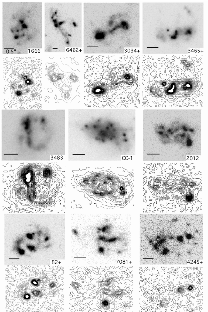
Figure 1: Grayscale i-band images and contour plots for 10 clump-cluster galaxies. The bar indicates $0.5^{\prime\prime}$; galaxy UDF names are noted. The contours are linear in steps of 1 $\sigma$ sky noise, with the outermost contour at 26.8 mag arcsec^-2.

Figure 1 shows 10 of the most spectacular clump clusters seen at i₇₇₅-band. They were chosen because of their large angular size, good resolution into clump and interclump regions, and wide range of feature types representing most galaxies in this class. Their positions and integrated properties are in Table 1. Some have multiple UDF numbers because SExtractor identified the individual large clumps as separate sources. Contour plots of intensity are drawn with the lowest contour 1$\sigma$ above sky noise, corresponding to a surface brightness of 26.8 mag arcsec^-2 at i₇₇₅-band. The lower left-hand bar in each panel represents 0.5 arcsec. The numbers in the lower right are the UDF catalog numbers.

Objects UDF 3483 and UDF 82+99+103 are ring-like galaxies, while UDF 7081+7136+7170, UDF 4245+4450+4466+4501+4595, UDF 3034+3129, UDF 3465+3597, and UDF 3483 have linear central sections resembling bars (Paper III). UDF 4245+ also has several small clumps distributed around the periphery, while galaxy CC-1 has many small clumps throughout the body. UDF 2012 apparently has a dust lane running through the middle.

The integrated galaxy magnitude was measured in a rectangular box with edges defined by the i₇₇₅ isophotal contours $2\sigma$ above the sky noise for each filter (corresponding to a surface brightness of 26.0 mag arcsec^-2). We also did photometry on each prominent clump and several interclump regions, giving surface brightnesses and colors. Clump photometry was done using $imstat$ in IRAF by measuring the total flux inside a box that surrounds the clump and then subtracting the adjacent background in the same size box. The background was based on several flux readings in the immediate neighborhood of the clump.

Bright clumps have surface brightnesses that are $\sim 1.5$ mag arcsec^-2 brighter than the interclump regions. On average, $\sim 40$% of the i-band luminosity is in the clumps, as indicated by the clump luminosity fractions, $f_{\rm lum}$, in Table 1. This luminosity fraction corresponds to a different rest-frame wavelength in each case because the galaxy redshifts differ, so it is only meant to be a indicator of the highly clumped morphology viewed at i-band. The two cases with small $f_{\rm lum}$, UDF 4245+ and CC-1, have many more clumps, and each is much smaller than in the other objects. Most clump colors within a given object are similar to each other, although some apparently dusty interclump regions are much redder than others, such as the dust lane in galaxy UDF 2012.

A color-magnitude diagram for i₇₇₅ versus i₇₇₅-z₈₅₀ is shown in Figure 2 for all of the big clumps in Figure 1 (circles) and for the sum of these clumps (small squares) and the integrated galaxies (large squares). The i₇₇₅ magnitudes of the clumps range from 25.4 to 30.5. The colors lie mostly in a narrow range for each galaxy but they vary from galaxy to galaxy with the redshift (see below).

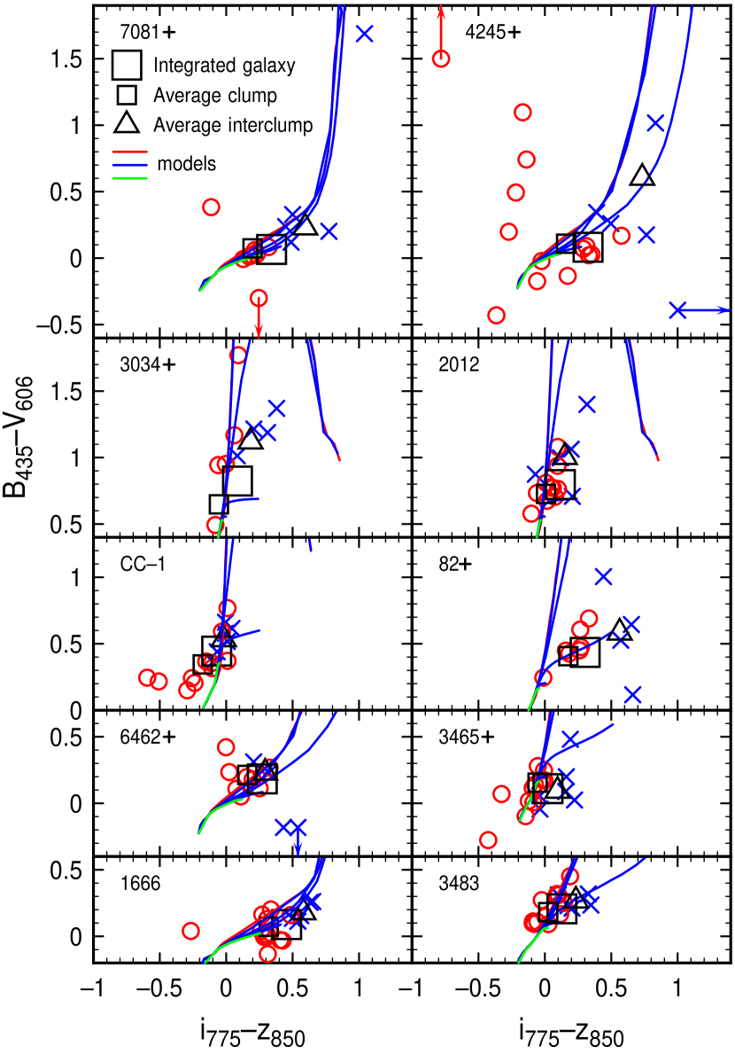
Figure 3: Color-color distribution of clumps (circles), interclump regions (crosses), and whole galaxies (squares). The average colors for the clumps (small squares) and interclump regions (triangles) are also shown. Curves are theoretical models that best match the fitted redshifts of the galaxies to the nearest 0.25. In general, the lower curves (bluer) correspond to the largest star formation decay times, which are assumed to be infinite (green curve for the electronic version of this publication), $10^{7}$ yr, $3\times 10^{7}$ yr, $10^{8}$ yr, $3\times 10^{8}$ yr, and $10^{9}$ yr (red curve). The best-fit models are determined simultaneously from both this color-color plot and the one in the next figure. Observed points that are far off the range of scales are indicated by arrows; they were not included in the model fits.

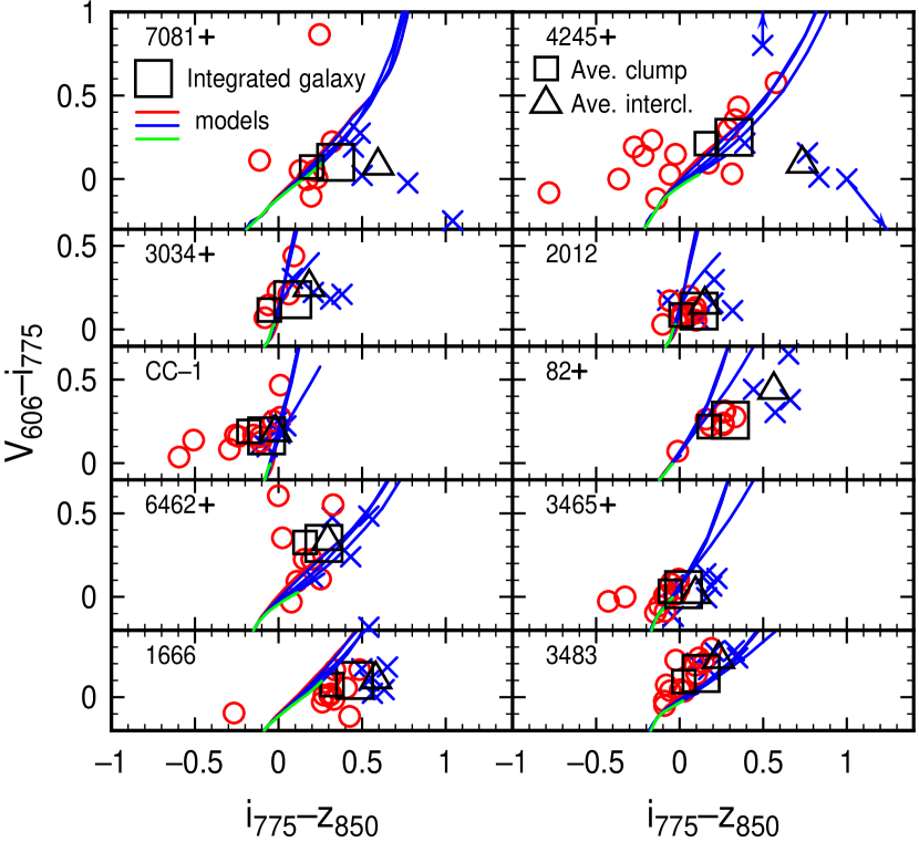
Figure 4: Color-color distribution of clumps (circles), interclump regions (crosses), whole galaxies (squares) and averages (small squares, triangles) are shown as in Figure 3, along with theoretical tracks that are closest in redshift to the fitted values.

Color-color diagrams for each clump-cluster galaxy are in Figures 3 and 4. The circles are the clumps, the crosses are the interclump media at various positions, the big squares are the integrated galaxies, the small squares are average colors of the clumps (weighted by clump luminosity), and the small triangles are the average weighted colors of the measured interclump emissions. Superposed curves are best-fit models that will be described in Section 3. The reddest B₄₃₅-V₆₀₆ colors are in UDF 3034+3129 and UDF 2012. In UDF 3034+3129, the central clump in the image has B₄₃₅-V${}_{606}=1.8$ mag, in UDF 2012, most of the red interclumps at B-V$>1$ mag are in the dust lane. Also very red (B₄₃₅-V${}_{606}=1.1$ mag) is the large western clump in UDF 4245+, which has a similarly red interclump region. The two bluest clumps in B₄₃₅-V₆₀₆ are in UDF 7081+ (the southernmost round clump) and UDF 2012 (the central clump just above the dust lane). The bluest clump in $i_{775}-z_{850}$ is in CC-1, and is a faint clump in the southeast. Figures 3 and 4 show that the interclump regions are systematically redder than the clumps.

3 Comparison with models

3.1 Model Components

Photometric redshifts for the 10 clump-cluster galaxies and the ages and luminous masses of the clumps and interclump regions were determined by comparison with stellar population models. The luminous mass is defined to be the mass that fits the observed emission in the bandpasses we have available. This mass does not include possible contributions from older populations of stars that do not emit significantly in the observed bandpasses and are not modelled explicitly in the star formation history.

The models used the GALAXEV tables of spectra in Bruzual & Charlot (2003) for the Padova1994 evolutionary tracks with a Chabrier (2003) IMF (extending from 0.1M_⊙ to 100 M_⊙ with a flattening below $\sim 0.5$ M_⊙). These tables give integrated population spectra at 1221 wavelengths from 91 Å to 160 $\mu$m and at 221 times from $1.25\times 10^{5}$ years to $2\times 10^{10}$ years. We use the low-resolution version. The spectra were integrated over time with two basic time dependencies for star formation, a constant rate, and an exponentially decreasing rate with timescales of $10^{7}$, $3\times 10^{7}$, $10^{8}$, $3\times 10^{8}$, and $10^{9}$ years. A choice of six metallicities is available in GALAXEV. Shapley et al. (2004) found that the metallicities for 7 disk galaxies at the same redshifts as those found here ($z\sim 2-2.5$) are approximately solar ($Z=0.02$). The metallicity of the Milky Way thick disk, which may have formed at about this epoch (Dalcanton & Bernstein 2002; Brook et al. 2004) peaks at $[{\rm Fe/H}]\sim=-0.6$ ($Z=0.005$). We use $Z=0.008$ in what follows; different metallicities did not change the results significantly.

Absorption from cosmological hydrogen lines was included according to the prescription in Madau (1995), taking Lyman series lines up to order 20 and including continuum absorption. Figure 5 shows the resulting transmission for a source at $z=3.5$ for comparison with Figure 3 in Madau (1995). Dust absorption was included using the wavelength dependence in Calzetti et al. (2000) with the short-wavelength modification in Leitherer et al. (2002) and the redshift dependence for galaxy intrinsic $A_{V}$ extinction in Rowan-Robinson (2003). The resulting rest-frame dust transmissions for galaxies at $z=1$ and $z=3.5$ are shown in Figure 6. Other estimates of extinction in $z\sim 2$ disk galaxies are 2 or 3 times higher than these (e.g., Adelberger & Steidel 2000; Papovich, Dickinson, & Ferguson 2001), so two other sets of models with twice and four times the Rowan-Robinson extinction were fit to our data for comparison, as discussed below. In general, higher extinction lowers the age and mass-to-luminosity ratio as the intrinsic stellar populations become bluer and brighter, but the masses may either increase or decrease depending on the relative size of the changes in $M/L$ and $10^{0.4A}$ for extinction $A$; the redshift solutions do not change noticeably with extinction over this range.

3.2 Model color evolution

The time-integrated spectra, corrected for cosmological hydrogen absorption and intrinsic galactic dust, were convolved with the four throughput functions for B₄₃₅, V₆₀₆, i₇₇₅, and z₈₅₀ filters, as determined from the IRAF task SYNPHOT (kindly run for us by Jennifer Mack at STScI). Equation 8 in the postscript file supplement of the GALAXEV download was used in the AB magnitudes convention. Because this AB version was not written explicitly for intensity as function of wavelength, we give it here:

$$m=-2.5\log\left[{{\int_{-\infty}^{\infty}d\lambda\lambda{{L_{\lambda}\left[\lambda\left(1+z\right)^{-1}\right]}\over{\left(1+z\right)c4\pi d_{L}^{2}}}F(\lambda)}\over{\int_{-\infty}^{\infty}{{d\lambda}\over{\lambda}}F(\lambda)}}\right]-48.60.$$ (1)

To get the constants of proportionality, the luminosity $L$ in GALAXEV, which is tabulated in units of L_⊙ $\AA^{-1}$ for each solar mass of stars, was converted to erg s^-1 $\AA^{-1}$ using $L_{\odot}=3.826\times 10^{33}$ ergs s^-1; $c$ is the speed of light in cm s^-1, $d_{L}$ is the luminosity distance in cm. The filter function, $F(\lambda)$, is dimensionless, as is $d\lambda/\lambda$ in the denominator. The combination $d\lambda L_{\lambda}$ has dimensions of ergs when $\lambda$ is in $\AA$, but the other $\lambda$ in the numerator has to be converted to cm to give $\lambda/c=1/\left(3\times 10^{18}\right)$ s¹; $\lambda$ is the observed wavelength.

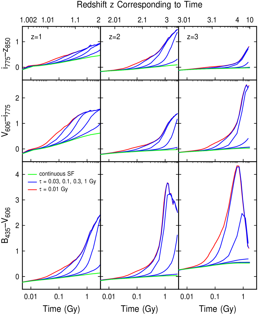
Figure 7: Model colors versus population age for three galaxy redshifts, $z=1$, 2, and 3, and six models of the star formation history, as in Figure 3. Redshifts corresponding to the population ages for given galaxy redshifts are on the top axis. The ticmarks for these redshifts are not the same interval throughout, but they should still be self-evident; for example, on the top left, the ticmarks are at 1.002, 1.003, 1.004, etc., to 1.01, and then 1.01, 1.02, 1.03, etc. to 1.1, and then 1.1, 1.2, 1.3, etc. to 2.

Models of color versus time are in Figure 7 for three values of redshift and for the six star formation histories. The lower curve in each panel (bluest color) is for continuous star formation and the upper curve (reddest color) is for the most rapidly decaying star formation, with an exponential decay time of 10 My. Intermediate curves span the range of exponential decay times, $\tau$, indicated in the figures. The colors rise with time rapidly, especially at high redshift, because of the depletion of uv light in the absence of current star formation. The Lyman absorption jump shown in Figure 5 reddens the B₄₃₅-V₆₀₆ values for all of the curves when $z>3.5$ (the drop-out effect – Steidel et al. 1996). The redshifts of star formation corresponding to the times on the abscissae are indicated on the top axes. Analogous models without intrinsic dust extinction differed only a little in color, at most $\sim 0.1$ mag in B₄₃₅-V₆₀₆.

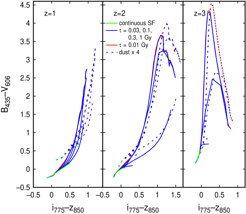
Figure 8: Population models on a color-color plot where time increases along each curve from the lower left to the upper right. The same six star formation histories as in the previous figures are used, with the same color coding. The solid lines are for internal extinction following the Rowan-Robinson (2003) result, and the dashed lines are for internal extinctions that are 4 times higher.

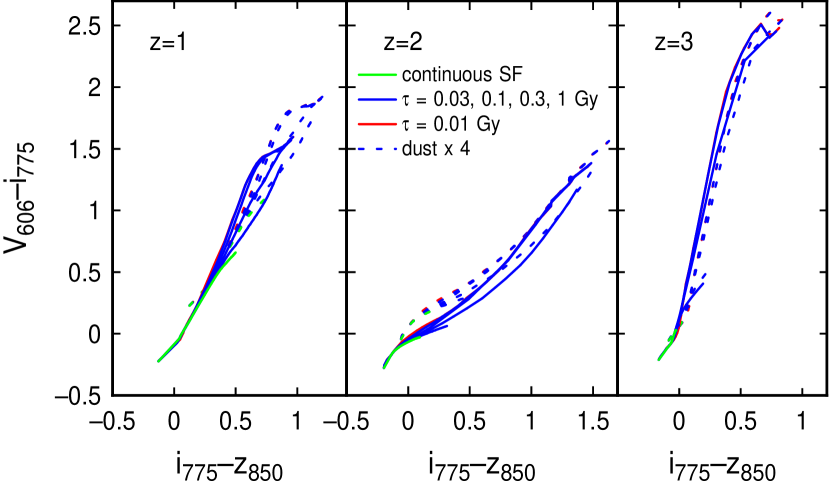
Figure 9: Model color-color plots as in Figure 8.

Model color-color plots are shown in Figures 8 and 9. Stellar age in the rest frame of the galaxy increases along the curves from 0 at the bottom left (bluest colors) to whatever age corresponds to $z\sim 8$ at the observed redshift (5.3 Gy, 2.7 Gy, and 1.5 Gy at $z=1$, 2, and 3, respectively). The different star formation histories have separate curves. Solid curves have dust extinction from Rowan-Robinson (2003) and dashed curves have 4 times this extinction. Generally, the more continuous the star formation, the closer the curve stays to the lower left end, even at large times. The most extreme red values occur for the most rapid decay, where the exponential time is $\tau=10$ My.

3.3 Photometric redshifts

The observed colors of the clump and interclump emissions correspond to the lower left parts of the theoretical color-color curves. Figures 3 and 4 show the data and models together, using the redshift models that best match the colors. To find these redshifts, we made models with the six star formation histories mentioned above and with redshifts ranging from $z=0$ to 6.75 in intervals of $z=0.25$. Model colors were tabulated for a wide range of times within each history type. The rms deviations between the average clump positions and the models on both color-color plots were then determined for each clump-cluster galaxy, and the model with the minimum rms was chosen. The highly deviant colors shown by arrows in the figures were not used for this. Thus the photometric redshifts are based only on the clump colors, not the average galaxy colors or the interclump emission. We do this because clumps are more homogeneous than whole galaxies. The fit to the redshift also gives the preferred star formation decay time, $\tau$, and the average age of the clumps in each object.

We solved for the three main variables (redshift, decay time, age) in a certain way to minimize possible variations from intrinsic scatter in the data. We first solved for the minimum value of $\delta=(bv-bv_{m})^{2}+(vi-vi_{m})^{2}+(iz-iz_{m})^{2}$ along each curve that traces out age for a given redshift and star formation history. This minimum was found by a quadratic fit to the lowest three $\delta$ values along that curve. Here, $bv$, $vi$, and $iz$ represent the observed colors and $bv_{m}$, $vi_{m}$ and $iz_{m}$ represent the model colors. Next, the minimum values of $\delta$ were arranged in order of increasing redshift and, for each redshift, increasing $\log(\tau)$ in the star formation history. Along this list there were usually one or two broad minima in the $\delta$ values, corresponding to close fits between the observed and model colors. Typically one close fit was at low $z$ and another was at intermediate-to-high $z$. This duplicity corresponds to the looping structure of the color-color curves in Figure 8, i.e., the template spectra have the same slope at two distinct wavelengths (typically at the rest optical and rest uv) for some star formation histories and extinctions. We could rule out the small-$z$ solutions because these gave effective rotation curve speeds (see below) that are unreasonably low for disk-like galaxies (i.e., 20 km s^-1 or less). The broad minima along the ordered models were then isolated from each other by considering only $\delta$ values less than certain limits, 0.1, 0.05, and 0.02. For each limit, the mean and the standard deviation of the $z$ value was determined, weighted by the inverse of $\delta$. When this mean $z$ was about the same for each limit, and the standard deviation in $z$ became small, $\pm 0.2$ or less, for the smallest limit, then we felt confident in our $z$ solutions.

The redshifts based on the whole galaxy colors were typically several tenths smaller than the redshifts based on the average clump colors. This difference is larger than the standard deviation for each $z$ and also larger than the differences in fitted $z^{\prime}s$ for the three limiting $\delta$ values. Most likely, the interclump emission, which contains about half the total light, is contributing to the composite galaxy spectrum in a way that makes the composite colors inconsistent with a single exponential-decay model for star formation. For example, whole galaxies are redder than clumps in i₇₇₅-z₈₅₀, and the models in Figure 8 shift i₇₇₅-z₈₅₀ toward the red for lower $z$. We believe that the fits to the clump colors give more accurate redshifts as long as we use simple star formation histories.

For each fitted $z$, we also got the inverse-$\delta$ weighted mean of $\log(\tau)$ in the star formation history and the inverse-$\delta$ weighted mean of the age of the star formation region, $t$.

To check our method, we compared the photometric redshifts derived from our models with the 19 published redshifts available for the GOODS field (Vanzella et al. 2004) using the photometry in that study and the same filters as the UDF field. We also compared our redshifts to those derived by Benitez et al. (2004) in the Tadpole Galaxy field, using the different filters appropriate to the Tadpole Galaxy survey. Figure 10 shows a plot of these redshift distributions. Our values matched the GOODS redshifts, which range from 0.21 to 1.4, with an rms deviation of 0.2, not counting an object at $z=5.83$, for which we derived $z=2.5$. This single large discrepancy could result from strong emission lines in the observation that are not present in the models, or from inappropriate models at high $z$. Our values matched the 107 high-quality photometric redshifts in the Tadpole field (i.e., those for which ODDS$>0.99$) to within an rms of 0.3, not counting 29 more for which Benitez et al. derived a redshift of around $1.85$. These excluded galaxies (not plotted) form a cluster in the redshift distribution with a value of $z$ from Benitez et al. $\sim 1.872\pm 0.015$; our redshifts for them range from 0.3 to 2.1, with an average of $1.28\pm 0.43$. Aside from these unexplained discrepancies, our photometric redshifts are comparable to the redshifts derived by others to within several tenths. We also determined redshifts for 30 B-band dropout galaxies in the UDF field (Elmegreen et al. 2005) and obtained an average of $3.49\pm 0.37$, which is reasonable.

The interclump age could not be derived reliably from our models because of the ambiguity between age and decay time $\tau$. The interclump emission is probably a composite of many ages, however, going back to the beginning of Pop II star formation, regardless of the nature of the galaxies in which these stars formed. To find the best interclump star formation histories, we used the galaxy redshifts found from the clump colors and assumed an interclump age corresponding to a beginning of interclump star formation at $z=6$. We then determined the value of $\tau$ for each galaxy that best fits the average three interclump colors.

3.4 Redshift and age solutions

Table 2 shows the main results of the fitting procedure with the Rowan-Robinson extinctions. The average clump age is derived to be 0.34 Gy from the clump colors and models. The average interclump age is assumed to be the time between the Universe age at the fitted clump redshift and the Universe age at $z=6$, when the interclump star formation presumably began. The average value in Table 2 is 2.14 Gy. This larger age for the interclump region is not unreasonable considering the redder colors there. The clumps are characterized by a decaying star formation rate with an e-folding time that has an average $\tau\sim 0.1$ Gy. Thus the clumps are three times older than their e-folding times and should not be considered starbursts. The fitted e-folding times for star formation in the interclump regions average $\sim 1$ Gy, which is only slightly less than the average interclump age and consistent with a continued build-up of these regions.

Extinctions E(B-V) larger than the Rowan-Robinson (2003) values by factors of 2 and 4 for both clump and interclump emission give about the same redshifts for the galaxies. The average values for various quantities in these two cases are given in the bottom rows of the tables. The average redshift decreases from $z=2.3$ with our fiducial extinction to 2.2 for both $2\times$ and $4\times$ extinctions. The higher extinctions decrease the average clump ages from 0.34 Gy to 0.23 Gy and 0.09 Gy, respectively, with $<\tau>=0.17$ and $0.16$ for the two cases, because the source has to be intrinsically bluer when there is additional reddening. They also make the interclump regions intrinsically bluer by increasing the star formation decay times, $\tau$, from an average of 1.01 Gy to averages of 2.09 Gy and 3.30 Gy, respectively.

The redshifts allow the determination of the luminosity distance $d_{L}$ in equation 1 (Carroll, Press, & Turner 1992). The resulting model apparent magnitudes scaled to the observed apparent magnitudes give the clump masses. This derivation of mass uses the evolution models in GALAXEV again, as they give the residual stellar mass per initial solar mass of a population of stars as a function of time. To get the clump mass, we integrated this residual stellar mass over time using the same time-dependent star formation rate as for the integrated spectrum, and then multiplied the resultant model mass by the factor used to scale the model luminosity to the observed clump luminosity.

3.5 Interclump mass column densities

The interclump mass column densities were obtained from the observed interclump surface brightnesses. To be careful about surface brightness dimming, we first wrote the absolute magnitude of a solar mass of stars from equation 1 using $d_{L}=10$ pc. We then used the cosmological distance modulus (Carroll, Press, & Turner 1992; Paper III) to give the apparent magnitude for this solar mass and scaled this result to the observed apparent magnitude in a square arcsec. This gave the mass per square arcsec. The square arcsec was then converted into a square kiloparsec using the cosmological angle formula (Carroll, Press, & Turner 1992) to get the rest-frame mass column density. This process corrects for the $\left(1+z\right)^{4}$ surface brightness dimming. We got the same result using the $z$-dependent luminosity distance $d_{L}$ in equation 1. The total interclump mass was determined by averaging the interclump masses per square arcsec for each galaxy and multiplying this average by the galaxy area in square arcsecs. This assumes the interclump medium is uniform. The interclump mass column density is typically larger than the clump mass column density. Evidently, the clump light is dominated by the brightest blue stars, while the total mass in the region is dominated by the underlying old stars. The sum of the clump mass and the interclump mass is taken to be the luminous galaxy mass.

3.6 Results

Table 3 gives the average clump mass, $<M_{\rm clump}>$, diameter $<D_{\rm clump}>$, and clump mass fraction, $f_{\rm mass},$ in each clump-cluster galaxy, and it gives the luminous galaxy mass, $M_{\rm gal}$, the galaxy diameter, $D_{\rm gal}$ (equal to the major axis length out to the 2-$\sigma$ contour), and the effective rotation speed, $v_{\rm rot}=\left[GM_{\rm gal}/\left(5D_{\rm gal}/2\right)\right]^{1/2}$ (the factor 5 in the denominator assumes a uniform spherical mass distribution). For the physical sizes, $D$, the angular sizes were used along with the cosmological angle-size relation for the galaxy redshift.

The results in Table 3 may be summarized as follows. The objects we have selected are large composite systems with an average luminous mass of $6.5\times 10^{10}$ M_⊙ and an average diameter of 19.1 kpc out to the 2$\sigma$ contour. The size and mass are not unprecedented for disk galaxies at redshifts of 2 to 3 (Labbé et al. 2003; Shapley et al 2004). The average rotation speed would be 150 km s^-1 if there were regular circular motion, but there are no spectroscopic observations yet. There is a range of a factor of 50 in mass and a factor of 8 in rotation speed, so the peculiar morphology of this galaxy type does not correspond to a particular mass. The clumps represent an average total mass fraction of 19%, again with a factor of 10 variation. This is smaller than their luminosity fraction mentioned above (40%) because the older interclump medium has a higher mass-to-light ratio than the clumps.

The average interclump mass column density is $\sim 4$ times larger than the mass column density in solar neighborhood. The primary reason for the high value is the red color of the interclump stars. Colors this red are matched to stellar populations with high mass-to-light ratios. Increasing the assumed dust abundance by factors of 2 and 4 for both the clumps and the interclump regions hardly changed the redshifts and also changed the clump masses only a little, from an average of $0.64\times 10^{9}$ M_⊙ to averages of $0.97\times 10^{9}$ M_⊙ and $0.53\times 10^{9}$ M_⊙, respectively. These small changes reflect the close balance between decreasing $M/L$ ratios for intrinsically bluer stars and increasing $\exp\left(\tau_{\rm dust}\right)$ corrections for more reddened stars. The interclump masses and total galaxy masses changed with extinction only a little too: the average total galaxy masses changed from $6.5\times 10^{10}$ M_⊙ to $6.4\times 10^{10}$ M_⊙ $11\times 10^{10}$ M_⊙, respectively. Lower metallicity would also make the intrinsic colors bluer, and this would make the interclump ages older to match the observed colors, producing an even higher $M/L$. Changes in the stellar initial mass function could lower the inferred interclump mass, but only if the relative abundance of stars younger than $\sim 1$ Gy, corresponding to A-type stars or earlier, is higher in proportion to low mass stars than found locally; i.e., the IMF has to be relatively flat at intermediate to high mass.

In another series of models, we assumed the Rowan-Robinson (2003) extinction for the models of the clump emission, getting the same clump redshifts and ages as before, but then we assumed higher extinctions in the interclump regions by factors of 2 and 4 before deriving their star formation histories and masses. These higher interclump extinctions gave intrinsically bluer colors and a greater extinction correction to the magnitudes. The resultant interclump masses averaged for all 10 galaxies increased from $5.9\times 10^{10}$ M_⊙ to $6.5\times 10^{10}$ M_⊙ $12\times 10^{10}$ M_⊙ respectively, as the corresponding lower mass-to-luminosity ratios were more than offset by a higher mass needed to overcome the greater extinction.

Other clump properties are in Table 4. The clump equivalent atomic density, $n_{\rm clump}$, is taken to be the ratio of the clump stellar mass to the volume given by the clump diameter, $D_{\rm clump}$, assuming a mean molecular weight $2.2\times 10^{-24}$g. This equivalent density is useful for comparisons with molecular cloud and other gas densities (see below). The dynamical time is $t_{\rm dyn}=\left(G\rho\right)^{-1/2}$ for mass density $\rho$. The average and current star formation rates (SFR) are given by

$${\rm SFR(ave)}=M_{\rm clump}/t\;\;;\;\;{\rm SFR}={{M_{\rm clump}e^{-t/\tau}}\over{\tau\left(1-e^{-t/\tau}\right)}}$$ (2)

for clump age $t$ and decay time $\tau$ in Table 2. The internal clump velocity dispersion assumes virial equilibrium with a uniform density: $\Delta v_{\rm clump}=\left[GM_{\rm clump}/\left(2.5D_{\rm clump}\right)\right]^{1/2}$. The last column is the ratio of the clump internal dynamical time to the galaxy dynamical time. All of these properties are discussed below.

4 Discussion

4.1 General considerations

Clump-cluster galaxies are a new type of object seen primarily in deep fields such as those surveyed by HST. They are characterized by: (1) a disk-like shape (Paper II); (2) a significant contribution to the total luminosity ($\sim 40$% – Table 1) from a small number of relatively blue clumps; (3) a flat light profile along the major axis (Papers I, II); (4) no central red clump or bulge (Papers I, II); and (5) a faint, relatively red interclump emission (this paper). Some clump-clusters also have bar-like features (Paper III). Edge-on clump-clusters may be chain galaxies (Paper II). The lack of clear rotation in chain galaxies (Bunker et al. 2000; Erb et al. 2004) is a mystery if these are normal galaxy disks.

In the few cases studied here, the clumps are typically $\sim 0.3$ Gy old in their rest frame and not currently forming stars as fast as they once did. Emission from the interclump medium is dominated by stars that are much older, perhaps up to 2 Gy older in some cases. Older and fainter populations inside the clumps could be present but undetected.

With $\sim 19$% of the luminous mass in a dozen or so giant clumps, these galaxies are unlike modern galaxies where the largest star forming regions are typically $<10^{-4}$ of a galaxy’s mass. This difference implies several things. First, the extreme clumpiness suggests that the rotation curve will not be simple (Immeli et al. 2004a,b). The clumps should attract each other and scatter, with their coldest and most dissipative parts migrating to the center to make a bulge and their hottest, least dissipative parts filling the interclump region or thick disk (Noguchi 1999; Somerville, Primack & Faber 2001; Immeli et al. 2004a,b; Hartwick 2004; Brook et al. 2004). The lack of clear rotation in the few chain galaxies that have been observed may be the result of this severe clump interaction.

Second, the clump ages are longer than their dynamical times, so the clumps are self-bound like giant clusters. The clump density is comparable to the mean galaxy density, however, so tidal forces on the clumps are significant (this follows from the comparable clump and galaxy dynamical times in Table 4). This means that galactic shear and tidal stretching are moderately important for the lowest density clumps. For example, UDF 6462+6886 and UDF 82+99+103 have clumps with tails and arcs suggesting the influence of tidal forces.

The fact that the equivalent clump atomic densities are much less than typical molecular cloud densities implies that the clump stars probably formed in numerous dense cores inside kpc-size, gravitationally-bound, low-density cloud complexes. This hierarchical morphology for star formation is analogous to the case of star complexes found in local spiral galaxies (Efremov 1995), except that for the clump clusters, the clumps are more strongly bound; local star complexes readily disperse or shear into flocculent spiral arms.

The internal velocity dispersions in the clumps are inferred to be moderately large, 24 km s^-1 on average, based on the virial theorem. This velocity is $\sim 16$% of the average galactic orbital speed – a high fraction for gas in local spirals but comparable to the fraction in dwarf galaxies. If the clouds that made the young stellar clumps formed by gravitational instabilities (Noguchi 1999; Immeli et al. 2004a,b) and if they still have the ambient Jeans mass, then the velocity dispersion in the pre-cloud gas had to be comparable to the virial velocity in the clumps (this is based on the usual isothermal assumption). Such a high dispersion implies that clump-cluster galaxies are far more turbulent than local galaxies.

One source of turbulence could be major encounters with other galaxies. Tidal forces increase the velocity dispersion considerably in local galaxies undergoing such encounters (Kaufman et al. 1997). The galaxies in our sample have no major companions now, but the giant clumps in them could have been triggered $\sim 0.3$ Gy ago at previous encounters, considering the average clump age. Another possible source of turbulence is accretion from the intergalactic medium. The disk impact speed can be $\sim 0.4$ times the circular speed if the gas falls in along cosmological filaments (Keres et al. 2004). This would be $\sim 60$ km s^-1 for our galaxies. Disk turbulence should be slower than this because of energy dissipation, but still enough to explain the high $\Delta v_{clump}$. Supernovae could also be an important source of turbulence as they are in local galaxies, but in clump-cluster galaxies they are likely to be highly concentrated in the clumps, and then they may just cause blow-out rather than widespread turbulence.

In the accretion model, clump-cluster galaxies would have added intergalactic gas at a rate comparable to the average star formation rate, $\sim 20$ M_⊙ yr^-1. The disks would presumably have become unstable when the mass column density exceeded a critical value. Considering the clump ages, the resulting star formation has a timescale of $\sim 0.3$ Gy, which is several galactic orbit times.

4.2 Accretion models

A different possibility is that the clumps were formerly separate galaxies that accreted during hierarchical buildup (e.g., Abadi et al. 2003; Brook et al. 2004). Some of our clump clusters are so irregular in morphology (e.g., UDF 6462+6886) that they appear more like random conglomerations than circular disks. Also, the lack of clear rotation in the few cases observed suggest highly disturbed dynamics. This model raises three questions: (1) Can small galaxies like our clumps survive their capture by large galaxies, considering the interclump population that was present before? (2) Are there examples of bare clumps in the UDF that resemble the clumps in our sample? (3) Would the distribution of axial ratios for coalesced systems be the same as that observed for clump clusters and chain galaxies? We attempt to answer these questions here.

4.2.1 Clump Survival

The short-term survival of a small galaxy captured by a large galaxy depends mostly on the ratio of densities. This ratio is important because it is also the ratio of the self-binding force per unit length inside the small galaxy to the tidal disruptive force per unit length exerted by the large galaxy. If the small galaxy is much denser than the large galaxy, then the small galaxy will survive until it migrates, perhaps because of dynamical friction, to a sufficiently dense region of the large galaxy, at which time it disperses. The migration time depends on the orbit, and the outer parts of the clump can be shredded continuously as it migrates. In the clump-cluster galaxies studied here, the typical column density of a clump is comparable to the average column density of the interclump population, both being several hundred M_⊙ pc^-2. The clump density should be considerably higher than the interclump density, however, because the interclump medium is likely to be much thicker than any single clump as a result of stirring from clump motions, dissolution of previous clumps, and stellar migration. The ratios of axes for these galaxies also suggest fairly thick disks (Paper II, and see below). In addition, the clumps probably have dense cores like other bound clusters. The clumps are therefore likely to survive their first few impacts with the disk, but probably not much longer. The observation that the clumps are much older than both their internal dynamical times and the galaxy orbit times (by a factor of 10) implies that most of them live outside the densest regions of the disk. The exceptions are the clumps with morphologies suggesting tidal disruption, such as the head-tail shapes of the clumps in UDF 82+99+103, UDF 6462+6886, and UDF 3034+3129.

4.2.2 Bare clumps in the UDF

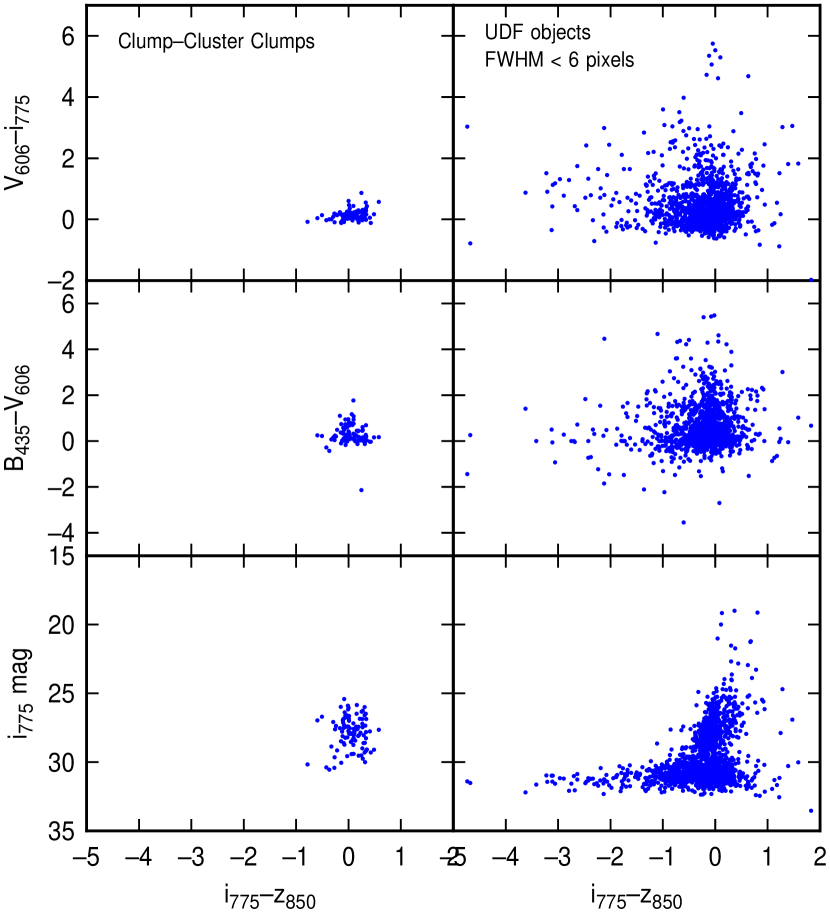
Figure 11: (left) Color-color and color-magnitude distributions for all the measured clumps in our 10 clump-cluster galaxies, and (right) analogous distributions for all the small clumps in the UDF field, with diameters less than 6 pixels. The similar distribution centroids suggest that the clumps in our clump-cluster galaxies could have been captured from the field. The faintest objects in the field also have faint counterparts in clump-cluster galaxies, but they were not included in our clump measurements.

What is the evidence for clumps like these outside of clump-cluster galaxies, where they presumably existed before the accretion? The UDF contains many isolated objects that resemble our clumps in both luminosity and color. The right-hand side of Figure 11 shows color-magnitude and color-color plots of all the UDF objects smaller than 6 pixels in FWHM, as given in the tabulation on the UDF web site. This size limit was chosen because it roughly corresponds to the size of a clump in a clump-cluster galaxy. The left side of the figure shows the magnitudes and colors for the measured clumps in the clump-cluster galaxies of this paper. The distributions are essentially the same in the regions of overlap. The UDF clumps can be much bluer than our clumps, suggesting either that star formation begins to slow down once a clump is ingested into a larger galaxy, or the clump-cluster sample in our survey has too few clumps to include the rare active ones seen in the general UDF field. There are also much fainter clumps in the UDF field than those measured in our survey, but the clump-cluster galaxies have much fainter clumps too which we did not study. We note that these small objects in the UDF field are not the well-studied Lyman Break galaxies, which tend to be more massive, blue, and luminous than our clumps even at the same $z\sim 2.5-3$ (e.g., Papovich, Dickinson, & Ferguson 2001). The small field objects are more the size of the $z\sim 6$ galaxies studied by Bunker et al. (2004). Most likely, most are low-mass and low-luminosity galaxies in about the same range of redshifts as the clump-cluster galaxies studied here.

4.2.3 Distribution of axial ratios

The distribution of axial ratios for a random assembly of field clumps might be expected to be significantly different than the distribution for a thick disk. This distribution was determined for a combined sample of chain and clump-cluster galaxies in Paper II and shown to be similar to the distribution for nearby spiral galaxies (see also O’Neil et al. 2000; Reshetnikov, Dettmar, & Combes 2003). In general, a thin disk should have a flat distribution for the ratio of minor to major axes, $W/D$, with a slight rise and then a drop at low ratios where the projected width $W$ becomes comparable to the intrinsic disk thickness. A galaxy whose appearance is dominated by a few clumps will not be very different, in fact. The first three clumps make a plane regardless of their positions, so the question is how much do the few additional clumps in a clump-cluster or chain galaxy distort this projected plane?

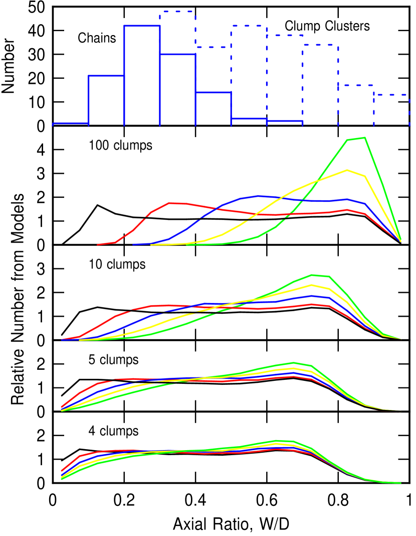
Figure 12: (top) The distribution of the ratio of minor to major axes for all the chain galaxies (solid line) and clump-cluster galaxies (incrementally represented by the dashed line) in our larger survey of the UDF field. The bottom 4 panels show models of axial ratios for pure-clump galaxies with randomly positioned clumps. In each case, there are 5 curves that correspond to intrinsic flattenings of $Z=0.1$, 0.3, 0.5, 0.7 and 1 (which is an unflattened spherical distribution). These curves move progressively to the right in the panels. The number of clumps in the models is different for each panel, as indicated. The figure shows how UDF galaxies dominated by 5 to 10 clumps, such as chain and clump-cluster galaxies, are most likely flattened with an intrinsic axial ratio of 0.1 to 0.3, as shown by the black and red curves (in the electronic edition) in the second and third panels up from the bottom. The decrease in the distribution at high axial ratio is from the intrinsically irregular structure of the galaxies (smooth disks would not have such a decrease), while the decrease at low axial ratio is from the minimum intrinsic flattening. Evidently, the clump-cluster galaxies are in the process of forming thick disks.

Figure 12 shows distribution functions of axial ratios for model galaxies with various numbers of clumps randomly positioned in 3 dimensions. Each line is a histogram from $10^{5}$ models. The first three clumps in each model are taken to define a plane and the others are given random positions around the plane in polar coordinates. The radial distance of each clump is distributed as a Gaussian. To simulate variations from different degrees of flattening in a disk, the distance perpendicular to the plane is multiplied by factors of $Z=0.1,$ 0.3, 0.5, 0.7, and 1 for the five different lines. Once a clump distribution is chosen, the polar axis of the model is tilted by a random angle whose cosine has a uniform distribution function, simulating random inclinations of the model in the sky. The axial ratio used for the histogram is then taken to be the minimum ratio of projected width to length, considering all angles in the sky plane. The resulting histograms peak for axial ratios near unity when $Z=1$ and there are a lot of clumps, because then the model galaxy is a uniformly filled sphere. When the number of clumps is small, the distribution decreases at high axial ratios because the clumps are irregularly positioned even in the spherical case ($Z=1$) and some directions happen to have have short sizes. The distributions decrease at small axial ratio because there are usually some clumps at non-zero perpendicular distance, making $W/D$ non-zero. The axial ratio where this decrease begins is smaller for more flattened systems because the minimum value of $W/D$ is $\sim Z$.

The observed distribution of axial ratios for all of the chains and clump-cluster galaxies in our survey of the UDF field (Elmegreen et al. 2005) is also shown in Figure 12. The solid line is for chains and the dashed line is for clump-clusters, added on top of the solid line. The observed distribution resembles the models only when there is some intrinsic flattening of the galaxies. However, the degree of flattening does not have to be large. The best models are for a number of clumps appropriate to our galaxies, $\sim 5-10$, and for a flattening $Z\sim 0.3$, which is the second curve from the left (red in the electronic version). The corresponding intrinsic axial ratio of the model galaxies is the same, $\sim 0.3$, which implies the disks are very thick. The same conclusion was reached in Paper II.

4.3 Assessment of accretion model

These considerations suggest that the clumps in some of our clump-cluster galaxies could have been accreted as whole objects from the field. They would probably survive for the required time, there are isolated field galaxies like them, and the clump-clusters are relatively thick disks. Some energy dissipation perpendicular to the disk had to occur to flatten the clump distribution to the observed axial ratio of 0.1 to 0.3, but dynamical friction from the observed interclump disk could have done this during the capture process.

This capture scenario is consistent with the model by Brook et al. (2004), who suggest that thick disks in spiral galaxies form quickly, in less than 1 Gy, as a result of mergers with a small number of $\sim 2\times 10^{9}$ $M_{\odot}$ clumps. Hartwick (2004) also notes the quick formation time of thick disks, and suggests that the pre-galactic clumps which make them could remain today, in part, as disk globular clusters.

A peculiarity of our sample is the high interclump surface density. If this result is correct, then it implies that the galaxies cannot simply age to form present-day spiral disks. Today’s disks either have high mass column densities along with massive bulges, or low mass column densities without prominent bulges. They do not have high mass column densities and no bulges, like our clump-clusters. One possibility is that a large fraction of the mass in clump-cluster disks will migrate inward to form a bulge. This migration would be accompanied by outward angular momentum transfer, and might result from spiral waves or repeated interactions, with bar formation a possible intermediate step. Another possibility is that clump-cluster galaxies merge to form elliptical galaxies. The likelihood of this is high considering their relatively large sizes and high redshifts where interactions are still frequent.

B.G.E. is supported by the National Science Foundation through grant AST-0205097. Support for D.M.E. was provided by the Salmon Fund of Vassar College.

Table 1: Properties of Galaxies

UDF ID Numbers	Position	i775	B435-V606	V606-i775	i775-z850	$\mu_{775}$	No.	$f_{\rm lum}$
	$3^{\rm h}$ $32^{\rm m},$ $-27^{\circ}$	mag				mag arcsec-2
82+99+103	$40.7472^{{\rm s}},$ $49^{\prime}$ $26.047^{\prime\prime}$	23.6	0.43	0.25	0.30	25.1	8	0.48
3034+3129	$37.8404^{{\rm s}},$ $47^{\prime}$ $56.390^{\prime\prime}$	24.0	0.82	0.18	0.08	24.6	5	0.44
2012	$35.9178^{{\rm s}},$ $48^{\prime}$ $17.216^{\prime\prime}$	24.3	0.80	0.11	0.12	25.0	10	0.38
3483	$36.3842^{{\rm s}},$ $47^{\prime}$ $47.125^{\prime\prime}$	23.4	0.20	0.14	0.13	24.5	12	0.30
3465+3597	$35.6573^{{\rm s}},$ $47^{\prime}$ $48.567^{\prime\prime}$	23.5	0.11	0.04	0.02	24.3	11	0.34
CC-1	$49.3154^{{\rm s}},$ $47^{\prime}$ $26.377^{\prime\prime}$	22.0	0.44	0.16	$-0.07$	23.9	11	0.13
4245+4450+	$28.9470^{{\rm s}},$ $47^{\prime}$ $37.730^{\prime\prime}$	22.6	0.08	2.75	$-2.18$	23.7	14	0.06
4466+4501+4595
1666	$41.3128^{{\rm s}},$ $48^{\prime}$ $21.154^{\prime\prime}$	23.9	0.09	0.10	0.45	25.2	13	0.39
7081+7136+7170	$38.9909^{{\rm s}},$ $46^{\prime}$ $56.265^{\prime\prime}$	24.5	0.06	0.10	0.34	25.9	8	0.38
6462+6886	$43.5596^{{\rm s}},$ $46^{\prime}$ $59.376^{\prime\prime}$	23.5	0.18	0.32	0.27	25.5	8	0.36

Table 2: Redshift and Star Formation Properties

Galaxy	redshift	Clump	Clump	Interclump	Interclump
Number	z	age, t (Gy)	decay $\tau$ (Gy)	age (Gy)	decay $\tau$ (Gy)
82+	2.5	0.36	0.11	1.71	0.33
3034+	3.0	0.21	0.10	1.24	0.58
2012	3.0	0.12	0.03	1.26	0.65
3483	2.2	0.26	0.05	2.02	1.63
3465+	2.4	0.22	0.06	1.80	1.06
CC-1	2.8	0.35	0.14	1.40	1.38
4245+	1.7	0.32	0.05	2.92	1.16
1666	1.6	0.81	0.28	3.15	0.91
7081+	1.6	0.43	0.10	3.13	0.92
6462+	1.8	0.31	0.06	2.82	1.49
averages =	2.3	0.34	0.10	2.14	1.01
ave, $A_{V}\times 2$ =	2.2	0.23	0.17	2.40	2.09
ave, $A_{V}\times 4$ =	2.2	0.09	0.16	2.32	3.30

Table 3: Derived Properties

Galaxy	$<M_{\rm clump}>$	$<D_{\rm clump}>$	$f_{\rm mass}$	$M_{\rm gal}$	$D_{\rm gal}$	$v_{\rm rot}$
Number	$10^{9}$ M⊙	kpc		$10^{10}$ M⊙	kpc	km s-1
82+	1.36	2.5	0.04	25	18	350
3034+	0.70	2.1	0.16	2.2	16	110
2012	0.17	1.5	0.07	2.5	13	130
3483	0.75	1.4	0.32	2.8	14	130
3465+	0.50	1.5	0.28	2.0	17	100
CC-1	0.96	1.3	0.07	15	25	230
4245+	0.21	2.1	0.59	0.5	22	44
1666	0.52	1.6	0.08	8.7	19	200
7081+	0.35	1.9	0.11	2.6	20	110
6462+	0.90	2.4	0.22	3.3	29	100
average =	0.64	1.8	0.19	6.5	19	150
ave, $A_{V}\times 2$ =	0.97	1.8	0.10	6.4	19	140
ave, $A_{V}\times 4$ =	0.53	1.9	0.07	11	19	180

Table 4: Other Clump Properties

Galaxy	$n_{\rm clump}$	$t_{\rm dyn}$	SFR(ave)	SFR(now)	$\Delta v_{\rm clump}$	$t_{\rm dyn}v_{rot}/D_{\rm gal}$
Number	cm-3	Gy	M⊙ yr-1	M⊙ yr-1	km s-1
82+	5.1	0.037	31	3.9	31	0.73
3034+	3.3	0.046	17	4.0	24	0.32
2012	2.6	0.052	14	1.1	14	0.53
3483	16	0.021	34	0.6	30	0.20
3465+	7.4	0.030	25	2.6	24	0.19
CC-1	24	0.017	31	7.0	35	0.15
4245+	1.1	0.081	9.3	0.1	13	0.17
1666	5.0	0.037	8.4	1.4	24	0.39
7081+	2.4	0.053	6.5	0.4	18	0.28
6462+	3.7	0.043	23	0.5	25	0.15
average =	7.0	0.042	20	2.2	24	0.31
ave, $A_{V}\times 2$ =	6.7	0.068	25	4.7	22	0.38
ave, $A_{V}\times 4$ =	2.6	0.090	42	30	15	0.79

Figure 2: Color-magnitude distribution for clumps (circles), for the sum of all clumps (small squares) and for the whole galaxy (big squares). Abbreviated galaxy names are indicated.

Figure 5: Transmission from foreground cosmological hydrogen clouds for a galaxy at redshift $z=3.5$ calculated using the method of Madau (1995).

Figure 6: Transmission from dust inside the model galaxies using the Calzetti et al. (2000) and Leitherer et al. (2002) extinction curves and the intrinsic $A_{V}$ extinction in Rowan-Robinson (2003). Dust produces less spectral structure and color variation than cosmological hydrogen absorption, so the redshifts derived here are not sensitive to internal extinction.

Figure 10: A comparison of redshifts calculated by different methods. On the bottom are photometric redshifts for the Tadpole Field galaxies calculated here (abscissa) versus the Benitez et al. (2004) photometric redshifts (ordinate). The filters appropriate for the Tadpole survey were used; 29 galaxies with Benitez et al. redshifts in a narrow range around 1.8 were omitted as they appear to be anomalous. On the top are photometric redshifts for galaxies in the GOODS field (abscissa) versus the Vanzella et al. (2004) spectroscopic redshifts (ordinate). The filters appropriate to the GOODS survey were used in this case; they are the same as the filters for the UDF survey.

References

- (1) Abadi, M.G., Navarro, J.F., Steinmetz, M., Eke, V.R. 2003, ApJ, 597, 21
- (2) Abraham, R., van den Bergh, S., Glazebrook, K., Ellis, R., Santiago, B., Surma, P., & Griffiths, R. 1996, ApJS, 107, 1
- (3) Adelberger, K.L., & Steidel, C.C. 2000, ApJ, 544, 218
- (4) Beckwith, et al. 2004, preprint
- (5) Benitez, N. et al. 2004, ApJS, 150, 1
- (6) Brook, C.B., Kawata, D., Gibson, B.K., & Freeman, K.C. 2004, ApJ, 612, 894
- (7) Bruzual, G. & Charlot, S. 2003, MNRAS, 344, 1000
- (8) Bunker, A., Spinrad, H., Stern, D., Thompson, R., Moustakas, L., Davis, M., & Dey, A. 2000, in Galaxies in the Young Universe II, ed. H. Hippelein & K. Meisenheimer (Berlin: Springer)
- (9) Calzetti, D., Armus, L., Bohlin, R.C., Kinney, A.L., Koornneef, J., & Storchi-Bergmann, T. 2000, ApJ, 533, 682
- (10) Carroll, S.M., Press, W.H., & Turner, E.L. 1992, ARAA, 30, 499
- (11) Chabrier, G. 2003, PASP, 115, 763
- (12) Conselice, C. 2004, astro-ph/0405102
- (13) Conselice, C., Grogin, N.A., Jogee, S., Lucas, R.A., Dahlen, T., de Mello, D., Gardner, J.P., Mobasher, B., Ravindranath, S. 2004, ApJ, 600, L139
- (14) Conselice, C.J., Blackburne, J.A., & Papovich, C. 2004, astroph/0405001
- (15) Cowie, L., Hu, E., & Songaila, A. 1995, AJ, 110, 1576
- (16) Dalcanton, J.J. & Bernstein, R.A. 2002, AJ, 124, 1328
- (17) Dalcanton, J.J., & Schectman, S.A. 1996, ApJ, 465, L9
- (18) Dickinson, M., Papovich, C., Ferguson, H.C., & Budavári, T. 2003, ApJ, 587, 25
- (19) Efremov, Y.N. 1995, AJ, 110, 2757
- (20) Elmegreen, D.M., Elmegreen, B.G., & Sheets, C. 2004, ApJ, 603, 74 (Paper I)
- (21) Elmegreen, D.M., Elmegreen, B.G., & Hirst, A.C. 2004a, ApJ, 604, L21 (Paper II)
- (22) Elmegreen, B.G., Elmegreen, D.M., & Hirst, A.C. 2004b, ApJ, 612, 191 (Paper III)
- (23) Elmegreen, D.M., et al. 2005, in preparation
- (24) Erb, D.K., Steidel, C.C., Shapley, A.E., Pettini, M., & Adelberger, K.L. 2004, 612, 122
- (25) Ferguson, H. C., Dickinson, M., & Williams, R. 2000, ARA&A, 38, 667
- (26) Hartwick, F.D.A. 2004, ApJ, 603, 108
- (27) Idzi, R. et al. 2004, ApJ, 600, L115
- (28) Immeli, A., Samland, M., Gerhard, O., & Westera, P. 2004a, A&A, 413, 547
- (29) Immeli, A., Samland, M., Westera, P., & Gerhard, O. 2004b, ApJ, 611, 20
- (30) Iono, D., Yun, M.S., & Mihos, J.C. 2004, ApJ, 616, 199
- (31) Kaufman, M., Brinks, E., Elmegreen, D. M., Thomasson, M., Elmegreen, B. G., & Struck, C., 1997, AJ, 114, 2323
- (32) Keres, D., Katz, N., Weinberg, D.H., & Davé, R. 2004, MNRAS, in press, astroph/0407095
- (33) Labbé, I., et al. 2003, ApJ, 591, L95
- (34) Leitherer, C., Li, I.-H., Calzetti, D., Heckman, T.M. 2002, ApJS, 140, 303
- (35) Madau, P. 1995, ApJ, 441, 18
- (36) Moustakas, L. et al. 2004, ApJ, 600, L131
- (37) Murali, C., Katz, N., Hernquist, L., Weinberg, D.H., & Davé, R. 2002, ApJ, 571, 1
- (38) Noguchi, M. 1996, ApJ, 514, 77
- (39) O’Neil, K., Bothun, G.D., & Impey, C.D. 2000, ApJS, 128, 99
- (40) Papovich, C., Dickinson, M., & Ferguson, H.C. 2001, ApJ, 559, 620
- (41) Reshetnikov, V., Dettmar, R.-J., & Combes, F. 2003, A&A, 399, 879
- (42) Roche, N., Ratnatunga, K., Griffiths, R. E., & Im, M. 1997, MNRAS, 288, 200
- (43) Rowan-Robinson, M. 2003, MNRAS, 345, 819
- (44) Rudnick, G. et al. 2003, ApJ, 599, 847
- (45) Shapley, A.E., Steidel, C.C., Adelberger, K. L., Dickinson, M., Giavalisco, M., Pettini, M. 2001, ApJ, 137, 139
- (46) Shapley, A.E., Erb, D.K., Pettini, M., Steidel, C.C., & Adelberger, K.L. 2004, ApJ, 612, 108
- (47) Smith, A.M., et al. 2001, ApJ, 546, 829
- (48) Somerville, R.S., Primack, J.R., Faber, S.M. 2001, MNRAS, 320, 504
- (49) Sommer-Larsen, J., Götz, M., & Portinari, L. 2003, ApJ, 596. 47
- (50) Spergel, D.N., et al. 2003, ApJS, 148, 175
- (51) Steidel, C.C., Giavalisco, M., Dickinson, M., & Adelberger, K.L. 1996, AJ, 112, 352
- (52) Taniguchi, Y., & Shioya, Y. 2001, ApJ, 547, 146
- (53) van den Bergh, S., Abraham, R.G., Ellis, R.S., Tanvir, N.R.,Santiago, B.X., & Glazebrook, K.G. 1996, AJ 112, 359
- (54) Vanzella, E., Cristiani, S., Dickinson, M., Kuntschner, H., Moustakas, L. A., Nonino, M., Rosati, P., Stern, D., Cesarsky, C., Ettori, S., and 7 coauthors, 2004, astro-ph/0406591
- (55) Walker, I., Mihos, J., & Hernquist, L. 1996, ApJ, 460, 121
- (56) Westera, P., Samland, M., Buser, R., & Gerhard, O.E. 2002, A&A, 389, 761