Applications of Bayesian model selection to cosmological parameters

Abstract

Bayesian model selection is a tool to decide whether the introduction of a new parameter is warranted by data. I argue that the usual sampling statistic significance tests for a null hypothesis can be misleading, since they do not take into account the information gained through the data, when updating the prior distribution to the posterior. On the contrary, Bayesian model selection offers a quantitative implementation of Occam’s razor.

I introduce the Savage–Dickey density ratio, a computationally quick method to determine the Bayes factor of two nested models and hence perform model selection. As an illustration, I consider three key parameters for our understanding of the cosmological concordance model. By using WMAP 3–year data complemented by other cosmological measurements, I show that a non–scale invariant spectral index of perturbations is favoured for any sensible choice of prior. It is also found that a flat Universe is favoured with odds of $29:1$ over non–flat models, and that there is strong evidence against a CDM isocurvature component to the initial conditions which is totally (anti)correlated with the adiabatic mode (odds of about $2000:1$), but that this is strongly dependent on the prior adopted.

These results are contrasted with the analysis of WMAP 1–year data, which were not informative enough to allow a conclusion as to the status of the spectral index. In a companion paper, a new technique to forecast the Bayes factor of a future observation is presented.

1 Introduction

In the epoch of precision cosmology, we often face the problem of deciding whether or not cosmological data support the introduction of a new quantity in our model. For instance, we might ask whether it is necessary to consider a running of the spectral index, an extra isocurvature mode, or a non-constant dark energy equation of state. The status of such additional parameters is uncertain, as often sampling (frequentist) statistics significance tests do not allow them to be ruled out with high confidence. There is a large body of work that addresses the difficulties arising from the use of p–values (significance level) in assessing the need for a new parameter. Many weaknesses of significance tests are clarified, and some even overcome, by adopting a Bayesian approach to testing. In this work, we take the viewpoint of Bayesian model selection to determine whether a parameter is needed in the light of the data at hand.

The key quantity for Bayesian model comparison is the marginal likelihood, or evidence, whose calculation and interpretation is attracting increasing attention in cosmology and astrophysics (Drell et al., 2000; Saini et al., 2004; Lazarides et al., 2004; Beltran et al., 2005; Kunz et al., 2006; Trotta, 2007c), after it was introduced in the cosmological context by Jaffe (1996); Slosar et al. (2003). The marginal likelihood has proved useful in other contexts, as well, for instance consistency checks between data sets (Hobson et al., 2002; Marshall et al., 2006), the detection of galaxy clusters via the Sunayev-Zel’dovich effect (Hobson & McLachlan, 2003) and neutrino emissions from type II supernovae (Loredo & Lamb, 2002). In this paper we use the Savage–Dickey density ratio for an efficient computation of marginal likelihoods ratios (Bayes factor), while in a companion paper (Trotta, 2007a) we present a new method to forecast the Bayes factor probability distribution of a future observation, called PPOD (for “Predictive Posterior Odds Distribution”). We then illustrate applications to some important parameters of current cosmological model building.

This paper is organized as follows: we review the basics of Bayesian model comparison in section 2 and we introduce the Savage–Dickey density ratio (SDDR) for the computation of the Bayes factor between two nested models. Section 3 is devoted to the application of model selection to three central parameters of the cosmological concordance model: the spectral tilt of scalar perturbations, the spatial curvature of the Universe and a totally (anti)correlated isocurvature CDM contribution to the initial conditions. We discuss our results and summarize our conclusions in section 4.

Some complementary material is presented in the appendices. An explicit illustration of Lindley’s paradox is given in appendix A, the mathematical derivation of the SDDR is presented in appendix B while a series of benchmark tests for the accuracy of the SDDR are carried out in appendix C.

2 Bayesian model comparison

In this section, we first briefly review the basics of Bayesian inference and model comparison and introduce our notation. We then present the Savage–Dickey density ratio for a quick computation of the Bayes factor of two nested models.

2.1 Bayes factor

Bayesian inference (see e.g. Jaynes (2003); MacKay (2003)) is based on Bayes’ theorem, which is a consequence of the product rule of probability theory:

$$p({\theta}|{d},{M})=\frac{p({d}|{\theta},{M})\pi({\theta}|{M})}{p({d}|{M})}.$$ (1)

On the left-hand side, the posterior probability for the parameters ${\theta}$ given the data ${d}$ under a model ${M}$ is proportional to the likelihood $p({d}|{\theta},{M})$ times the prior probability distribution function (pdf), $\pi({\theta}|{M})$, which encodes our state of knowledge before seeing the data. In the context of model comparison it is more useful to think of $\pi({\theta}|{M}$) as an integral part of the model specification, defining the prior available parameter space under the model ${M}$. The normalization constant in the denominator of (1) is the marginal likelihood for the model ${M}$ (sometimes also called the “evidence”) given by

$$p({d}|{M})={\int_{\Omega}p({d}|{\theta},{M})\pi({\theta}|{M})\textrm{d}{\theta}}$$ (2)

where $\Omega$ designates the parameter space under model ${M}$. In general, ${\theta}$ denotes a multi–dimensional vector of parameters and ${d}$ a collection of measurements (data covariance matrix, etc), but to avoid cluttering the notation we will stick to the simple symbols introduced above.

Consider two competing models ${M}_{0}$ and ${M}_{1}$ and ask what is the posterior probability of each model given the data ${d}$. By Bayes’ theorem we have

$$p({M}_{i}|{d})\propto p({d}|{M}_{i})\pi({M}_{i})~{}~{}(i=0,1),$$ (3)

where $p({d}|{M}_{i})$ is the marginal likelihood for ${M}_{i}$ and $\pi({M}_{i})$ is the prior probability of the $i$th model before we see the data. The ratio of the likelihoods for the two competing models is called the Bayes factor:

$$B_{01}\equiv\frac{p({d}|{M}_{0})}{p({d}|{M}_{1})},$$ (4)

which is the same as the ratio of the posterior probabilities of the two models in the usual case when the prior is presumed to be noncommittal about the alternatives and therefore $\pi({M}_{0})=\pi({M}_{1})=1/2$. The Bayes factor can be interpreted as an automatic Occam’s razor, which disfavors complex models involving many parameters (see e.g. MacKay (2003) for details). A Bayes factor $B_{01}>1$ favors model ${M}_{0}$ and in terms of betting odds it would prefer ${M}_{0}$ over ${M}_{1}$ with odds of $B_{01}$ against 1. The reverse is true for $B_{01}<1$.

It is usual to consider the logarithm of the Bayes factor, for which the so–called “Jeffreys’ scale” gives empirically calibrated levels of significance for the strength of evidence (Jeffreys, 1961; Kass & Raftery, 1995), $|\ln B_{01}|>1;>2.5;>5.0$. Different authors use different conventions to qualify the Jeffreys’ levels of strength of evidence. In this work we will use the convention summarized in Table 1 – often in the literature one deems odds above $|\ln B_{01}|=5$ to be ‘decisive’, but we prefer to avoid the use of the term because of the strong connotation of finality that it carries with it. If we assume that the two competing models are exhaustive, i.e. that $p({M}_{0}|{d})+p({M}_{1}|{d})=1$ and a non–committal prior $\pi({M}_{0})=\pi({M}_{1})=1/2$, we can relate the strength of evidence to the posterior probability of the models,

$$p({M}_{0}|{d}) =\frac{B_{01}}{B_{01}+1}$$ (5)

$$p({M}_{1}|{d}) =\frac{1}{B_{01}+1}.$$

This probability is indicated in the third column of Table 1.

The subject of hypothesis testing has received an enormous amount of attention in the past, and the controversy on the subject is far from being resolved among statisticians. An illustration of the difference between Bayesian model selection and frequentist hypothesis testing is given in Appendix A, where Lindley’s paradox is worked out with the help of a simple example. There it is shown that the Bayesian approach has the advantage of taking into account the information provided by the data, which is ignored by frequentist hypothesis testing.

Table 1: Jeffreys’ scale for the strength of evidence when comparing two models, ${M}_{0}$ versus ${M}_{1}$, with our convention for denoting the different levels of evidence. The probability column refers to the posterior probability of the favoured model, assuming non–committal priors on the two competing models, i.e. $\pi({M}_{0})=\pi({M}_{1})=1/2$ and that the two models exhaust the model space, $p({M}_{0}|{d})+p({M}_{1}|{d})=1$.

$|\ln B_{01}|$	Odds	Probability	Notes
$<1.0$	$\,\raise 1.72218pt\hbox{$<$}\kern-8.00003pt\lower 2.6694pt\hbox{$\sim$}\,3:1$	$<0.750$	Inconclusive
$1.0$	$\sim 3:1$	$0.750$	Positive evidence
$2.5$	$\sim 12:1$	$0.923$	Moderate evidence
$5.0$	$\sim 150:1$	$0.993$	Strong evidence

Evaluating the marginal likelihood integral of Eq. (2) is in general a computationally demanding task for multi–dimensional parameter spaces. Thermodynamic integration is often the method of choice, whose computational burden can become fairly large, as it depends heavily on the dimensionality of the parameter space and on the characteristic of the likelihood function. In certain cosmological applications, thermodynamic integration can require up to 100 times more likelihood evaluation than parameter estimation (Beltran et al., 2005). An elegant algorithm called “nested sampling” has been recently put forward by Skilling (2004), and implemented in the cosmological context by Bassett et al. (2004); Mukherjee et al. (2006). While nested sampling reduces the number of likelihood evaluations to the same order of magnitude as for parameter estimation, in the cosmological context this does not necessarily imply that the computing time can be reduced accordingly, see Mukherjee et al. (2006) for details.

2.2 The Savage–Dickey density ratio

Here we investigate the performance of the Savage-Dickey density ratio (SDDR), whose use is very promising in terms of reducing the computational effort needed to calculate the Bayes factor of two nested models, as we show below (for other possibilities, see e.g. DiCiccio et al. (1997)).

Suppose we wish to compare a two-parameters model ${M}_{1}$ with a restricted submodel ${M}_{0}$ with only one free parameter, $\psi$, and with fixed $\omega=\omega_{\star}$ (for simplicity of notation we take a two–parameters case, but the calculations carry over trivially in the multi–dimensional case). Assume further that the prior is separable (which is usually the case in cosmology), i.e. that

$$\pi(\omega,\psi|{M}_{1})=\pi(\omega|{M}_{1})\pi(\psi|{M}_{0}).$$ (6)

Then the Bayes factor $B_{01}$ of Eq. (4) can be written as (see Appendix B)

$$B_{01}=\left.\frac{p(\omega|{d},{M}_{1})}{\pi(\omega|{M}_{1})}\right|_{\omega=\omega_{\star}}\quad{\text{(SDDR)}}.$$ (7)

This expression goes back to J.M. Dickey (1971), who attributed it to L.J. Savage, and is therefore called Savage–Dickey density ratio (SDDR, see also Verdinelli & Wasserman (1995) and references therein). Thanks to the SDDR, the evaluation of the Bayes factor of two nested models only requires the properly normalized value of the marginal posterior at $\omega=\omega_{\star}$ under the extended model ${M}_{1}$, which is a by–product of parameter inference. We note that the derivation of (7) does not involve any assumption about the posterior distribution, and in particular about its normality.

For a Gaussian prior centered on $\omega_{\star}$ with standard deviation $\Delta\omega$ and a Gaussian likelihood with mean $\hat{\mu}$ and width $\hat{\sigma}$, Eq. (7) gives

$$\ln B_{01}(\beta,\lambda)=\frac{1}{2}\ln(1+\beta^{-2})-\frac{\lambda^{2}}{2(1+\beta^{2})},$$ (8)

where we have introduced the number of sigma’s discrepancy $\lambda=|\hat{\mu}-\omega_{\star}|/\hat{\sigma}$ and the volume reduction factor $\beta=\hat{\sigma}/\Delta\omega$ (see Appendix A for details). For strongly informative data, $\beta^{-1}\gg 1$ and in terms of the information content $I=-\ln\beta\geq 0$, Eq. (8) is approximated by

$$\ln B_{01}\approx I-\lambda^{2}/2\quad\text{(informative data)}.$$ (9)

The two terms on the right–hand side pull the Bayes factor in opposite directions: a large information content $I$ signals a large volume of wasted parameter space under the prior, and acts as an Occam’s razor term favouring the simpler model, while a large $\lambda$ favours the more complex model because of the mismatch between the measured and the predicted value of the extra parameter. Evidence against the simpler model scales as $\lambda^{2}$, while evidence in its favour only accumulates as $I=-\ln\beta$. Furthermore, for strong odds against the simpler model ($\lambda\gg 1$) the prior choice becomes irrelevant unless $I\gg\lambda$, a situation which gives rise to Lindley’s paradox (see Appendix A). For the case where $\lambda\ll 1$, i.e. the prediction of the simpler model is confirmed by the observation, the odds in favour of the simpler model are determined by the information content $I$, and therefore by the prior choice.

The use of the SDDR for nested models has several advantages. A first important point is the analytical insight Eq. (7) gives into the working of model selection for two nested models, which we have briefly sketched above. Priors on the common parameters on both models are unimportant, as they factor out when computing the Bayes factor. The only relevant scales in the problem are the quantities $\lambda$ and $\beta$, see Eq. (9), with the latter controlled by the prior width on the extra parameter. The volume effect arising from a change in the prior (e.g., when enlarging the prior range) can be easily estimated from the SDDR expression, without recomputing the posterior. Usually, the posterior pdf in Eq. (7) will be obtained by Monte Carlo Markov Chain (MCMC) techniques. In this case, even a change in the variables, or a more restrictive prior can usually be applied by simply posterior re–weighting the MCMC samples without recomputing them. Secondly, the SDDR can be applied to existing MCMC chains, and therefore the model selection question can be dealt with easily after the parameter estimation step has already been performed. Finally, Appendix C demonstrates that in the benchmark Gaussian likelihood scenario the SDDR gives accurate results out to $\lambda\,\raise 1.72218pt\hbox{$<$}\kern-8.00003pt\lower 2.6694pt\hbox{$\sim$}\,3$. For larger value of $\lambda$ the performance of the method is hindered by the fact that it becomes very difficult with conventional MCMC methods to obtain samples far out into the tails of the posterior. One could argue however that the most interesting regime for model comparison is precisely where the SDDR can yield accurate answers. This is also the region where most of the model selection questions in cosmology currently lie. Finally, often a high numerical accuracy in the Bayes factor does not seem to be central for most model comparison questions, especially in view of the fact that the uncertainty in the result can be strongly dominated by the prior range one assumes. This suggests that a quick and computationally inexpensive method such as the SDDR might be helpful in assessing the model comparison outcome for a broad range of priors. We therefore advocate the use of SDDR method for model selection questions involving nested models with moderate discrepancies between the prediction of the simple model and the posterior result, $\lambda\,\raise 1.72218pt\hbox{$<$}\kern-8.00003pt\lower 2.6694pt\hbox{$\sim$}\,3$. We now turn to the demonstration of the method on current cosmological observations.

3 Application to cosmological parameters

In this section we apply the Bayesian model selection toolbox presented above to three cosmological parameters which are central for our understanding of the cosmological concordance model: the spectral index of scalar (adiabatic) perturbations, the spatial curvature of the Universe and an isocurvature cold dark matter (CDM) component to the initial conditions for cosmological perturbations.

3.1 Parameter space and cosmological data

We use the WMAP 3–year temperature and polarization data (Hinshaw et al., 2006; Page et al., 2006) supplemented by small–scale CMB measurements (Readhead et al., 2004; Kuo et al., 2004). We add the Hubble Space Telescope measurement of the Hubble constant $H_{0}=72\pm 8$ km/s/Mpc (Freedman et al., 2001) and the Sloan Digital Sky Survey (SDSS) data on the matter power spectrum on linear ($k<0.1h^{-1}\rm Mpc$) scales (Tegmark et al., 2004). Furthermore, we shall also consider the supernovae luminosity distance measurements (Riess et al., 2004). We denote all of the data sets but WMAP as “external” for simplicity of notation. We are also interested in assessing the changes in the model comparison outcome in going from WMAP 1–year to WMAP 3–year data. We shall therefore compare our results using the 3–year WMAP data with the first–year WMAP data release (Bennett et al., 2003; Hinshaw et al., 2003; Verde et al., 2003), complemented by the “external” data sets described above.

We make use of the publicly available codes CAMB and CosmoMC (Lewis & Bridle, 2002) to compute the CMB and matter power spectra and to construct Monte Carlo Markov Chains (MCMC) in parameter space. The Monte Carlo (MC) is performed using “normal parameters” (Kosowsky et al., 2002), in order to minimize non–Gaussianity in the posterior pdf. In particular, we sample uniformly over the physical baryon and cold dark matter (CDM) densities, $\omega_{b}\equiv\Omega_{b}h^{2}$ and $\omega_{c}\equiv\Omega_{c}h^{2}$, expressed in units of $1.88\times 10^{-29}~{}{\rm g/cm}^{3}$; the ratio of the angular diameter distance to the sound horizon at decoupling, $\Theta_{\star}$, the optical depth to reionization $\tau_{r}$ (assuming sudden reionization) and the logarithm of the adiabatic amplitude for the primordial fluctuations, $\ln 10^{10}A_{S}$. When combining the matter power spectrum with CMB data, we marginalize analytically over a bias $b$ considered as an additional nuisance parameter. Throughout we assume three massless neutrino families and no massive neutrinos (for constraints on these quantities, see instead e.g. Bowen et al. (2002); Spergel et al. (2006); Lesgourgues & Pastor (2006)), we fix the primordial Helium mass fraction to the value predicted by Big Bang Nucleosynthesis (see e.g. Trotta & Hansen (2004)) and we neglect the contribution of gravitational waves to the CMB power spectrum.

3.2 Model selection from current data

The scalar spectral index

As a first application we consider the scalar spectral index for adiabatic perturbations, $n_{S}$. We compare the evidence in favor of a scale invariant index (${M}_{0}:n_{S}=1$), also called an Harrison-Zel’dovich (HZ) spectrum, with a more general model of single-field inflation, in which we do not require the spectral index to be scale invariant, ${M}_{1}:n_{S}\neq 1$. The latter case is called for brevity “generic inflation”.

Within the framework of slow–roll inflation, the prior allowed range for the spectral index can be estimated by considering that $n_{S}=1-6\epsilon+2\eta$, where $\eta$ and $\epsilon$ are the slow-roll parameters. If we assume that $\epsilon$ is negligible, then $n_{S}=1+2\eta$. If the slow-roll conditions are to be fulfilled, $\eta\ll 1$, then we must have $|\eta|\,\raise 1.72218pt\hbox{$<$}\kern-8.00003pt\lower 2.6694pt\hbox{$\sim$}\,0.1$, which gives $0.8\,\raise 1.72218pt\hbox{$<$}\kern-8.00003pt\lower 2.6694pt\hbox{$\sim$}\,n_{S}\,\raise 1.72218pt\hbox{$<$}\kern-8.00003pt\lower 2.6694pt\hbox{$\sim$}\,1.2$. Hence we take a Gaussian prior on $n_{S}$ with mean $\mu=1.0$ and width $\sigma=0.2$.

The result of the model comparison is shown in Table 2. When employing WMAP 1–year data, the model comparison yields an inconclusive result ($\ln B_{01}=0.68\pm 0.04$), but the new, lower value for $n_{S}$ from the WMAP 3–year data, enhanced by the small scale CMB measurements and SDDS matter power spectrum data, does yield moderate evidence for a non–scale invariant spectral index ($\ln B_{01}=-2.86\pm 0.28$), with odds of about 17:1, or a posterior probability of a scale invariant index of 5%, when compared to the above alternative generic inflation model. This is a consequence of both the shift of the peak of the posterior to $n_{S}=0.95$ and a reduction of its spread when using WMAP 3–year data, which places the scale invariant value of $n_{S}=1$ at about $3.3\sigma$ away from the posterior’s peak (see however the discussion about possible systematic effects in Parkinson et al. (2006)). In Table 2 we also give the resulting value of the Bayes factor obtained by using the SDDR formula and a Gaussian approximation to the posterior, see Eq. (21). Since the marginalized posterior for $n_{S}$ is very well approximated by a Gaussian, we find a very good agreement between this crude estimate and the numerical result using the actual shape of the posterior, with a discrepancy of order $5\%$. This supports the idea that for reasonably Gaussian pdf’s using a Gaussian approximation to the SDDR might be a good way of obtaining a first estimate of the Bayes factor for nested models.

Our findings are in broad agreement with Parkinson et al. (2006), where it was found using nested sampling that a similar data compilation as the one employed here gives $\ln B_{01}=-1.99\pm 0.26$ for the comparison between the HZ model and a generic inflationary model with a flat prior between $0.8\leq n_{S}\leq 1.2$. For such a flat prior, we obtain, using the SDDR, $\ln B_{01}=-2.98\pm 0.28$, where the difference with Parkinson et al. (2006) has to be ascribed to different constraining power of the different data compilations used, rather than to the methods for computing the Bayes factor. For a more detailed discussion of a series of possible systematic effects which might change the outcome of the model comparison, see section IIIC in Parkinson et al. (2006).

Table 2: Summary of model comparison results from WMAP data combined with small–scale CMB measurements, SDDS, HST and SNIa data. WMAP3+ext refers to WMAP 3 year data release, WMAP1+ext to WMAP 1st year data. The most spectacular improvement from WMAP1 to WMAP3 is the moderate evidence against a scale–invariant spectral index. Errors in the Bayes factor are obtained by computing the variance of the SDDR estimate from 5 subchains (see Appendix C for details). The “estimate” column gives the value obtained by employing the Gaussian approximation to the likelihood, Eq. (21) for a Gaussian prior or Eq. (22) for a flat prior.

Data	$\ln B_{01}$ from SDDR		Odds in favour	Probability	Comment
	(numerical)	(estimate)	of simpler model	of simpler model
	Spectral index: $n_{S}=1$ versus $0.8\leq n_{S}\leq 1.2$ (Gaussian)
WMAP3+ext	$-2.86\pm 0.28$	$-3.00$	1 to 17	0.05	Moderate evidence for non–scale invariance
WMAP1+ext	$0.68\pm 0.04$	$0.71$	2 to 1	0.66	Inconclusive result
	Spatial curvature: $\Omega_{\kappa}=0$ versus $-1.0\leq\Omega_{\kappa}\leq 1$ (Flat)
WMAP3+ext	$3.37\pm 0.05$	$3.25$	29 to 1	0.97	Moderate evidence for a flat Universe
WMAP1+ext	$2.70\pm 0.09$	$2.68$	15 to 1	0.94	Moderate evidence for a flat Universe
	Adiabaticity: $f_{\text{iso}}=0$ versus $-100\leq f_{\text{iso}}\leq 100$ (Flat)
WMAP3+ext	$7.62\pm 0.02$	$7.63$	2050 to 1	0.9995	Strong evidence for adiabatic conditions
WMAP1+ext	$7.50\pm 0.03$	$7.53$	1800 to 1	0.9994	Strong evidence for adiabatic conditions

The spatial curvature

We now turn to the issue of the geometry of spatial sections. We evaluate the Bayes factor for $\Omega_{\kappa}=0$ (flat Universe) against a model with $\Omega_{\kappa}\neq 0$. As discussed above, we only need to specify the prior distribution for the parameter of interest, namely $\Omega_{\kappa}$. We choose a flat prior of width $\Delta\Omega_{\kappa}=1.0$ on each side of $\Omega_{\kappa}=0$, for we know that the universe is not empty (thus $\Omega_{\kappa}<1.0$, setting aside the case of $\Lambda<0$) nor largely overclosed (therefore $\Omega_{\kappa}\,\raise 1.72218pt\hbox{$>$}\kern-6.99997pt\lower 2.6694pt\hbox{$\sim$}\,-1$ is a reasonable range, see 3.3 for further comments).

Cosmic microwave background data alone cannot strongly constrain $\Omega_{\kappa}$ because of the fundamental geometrical degeneracy. Even CMB and SDSS data together allow for a wide range of values for the curvature parameter, which translates into approximately equal odds for the curved and flat models. Adding SNIa observations drastically reduces the range of the posterior, since their degeneracy direction is almost orthogonal to the geometrical degeneracy of the CMB. Further inclusion of the HST measurement for the Hubble parameter narrows down the posterior range considerably, since the handle on the value of the Hubble constant today breaks the geometrical degeneracy. When all of the data (WMAP3+ext) is taken into account, we obtain for the Bayes factor $\ln B_{01}=3.37\pm 0.05$, favouring a flat Universe model with moderate odds of about $29:1$ (see Table 2). This corresponds to a posterior probability for a flat Universe of 97%, for our particular choice of prior. We notice the slight improvement in these odds from the result obtained using WMAP1+ext data, where the odds were $15:1$, which is to be ascribed mainly to the inclusion of polarization data that helps further tightening constraints around the geometrical degeneracy.

The CDM isocurvature mode

The third case we consider is the possibility of a cold dark matter (CDM) isocurvature contribution to the primordial perturbations. For a review of the possible isocurvature modes and their observational signatures, see e.g. Trotta (2004). Determining the type of initial conditions is a central question for our understanding of the generation of perturbations, and has far reaching consequences for the model building of the physical mechanisms which produced them. Constraints on the isocurvature fraction have been derived in several works, which considered different phenomenological mixtures of adiabatic and isocurvature initial conditions (Pierpaoli et al., 1999; Amendola et al., 2002; Trotta et al., 2001, 2003; Trotta & Durrer, 2006; Bucher et al., 2004; Crotty et al., 2003; Valiviita & Muhonen, 2003; Beltran et al., 2004; Moodley et al., 2004; Kurki-Suonio et al., 2005). Two recent studies making use of the latest CMB data (Bean et al., 2006; Keskitalo et al., 2006) obtain different conclusions as to the level of isocurvature contribution. While both groups report a lower best fit chi–square for a model with a large ($n\sim 3$) spectral index for the CDM isocurvature component, they give a different interpretation of the statistical significance of the improvement. It is precisely in such a context that a model selection approach as the one presented here might be helpful, in that it allows to account for the Occam’s razor effect described above. The question of isocurvature modes has been addressed from a model comparison perspective by Beltran et al. (2005); Trotta (2007b).

Since the goal of this work is not to present a detailed analysis of isocurvature contributions, but rather to give a few illustrative applications of Bayesian model selection, we restrict our attention to the comparison of a purely adiabatic model against a model containing a CDM isocurvature mode totally correlated or anti–correlated. For simplicity, we also take the isocurvature and adiabatic mode to share the same spectral index, $n_{S}$. This phenomenological set–up is close to what one expects in some realizations of the curvaton scenario, see e.g. Gordon & Lewis (2003); Lyth & Wands (2003); Lazarides et al. (2004). For an extended treatment including all of the 4 different isocurvature modes, see Trotta (2007b).

We compare model ${M}_{0}$, with adiabatic fluctuations only, with ${M}_{1}$, which has a totally (anti)correlated isocurvature fraction

$$f_{\text{iso}}\equiv\frac{\mathcal{S}}{\zeta},$$ (10)

where $\zeta$ is the primordial curvature perturbation and $\mathcal{S}$ the entropy perturbation in the CDM component (see Trotta (2004); Lazarides et al. (2004) for precise definitions). The sign of the parameter $f_{\text{iso}}$ defines the type of correlation. We adopt the convention that a positive (negative) correlation, $f_{\text{iso}}>0$ ($f_{\text{iso}}<0$), corresponds to a negative (positive) value of the adiabatic–isocurvature CMB correlator power spectrum on large scales. We choose $f_{\text{iso}}$ as the relevant parameter for model comparison because of its immediate physical interpretation as an entropy–to–curvature ratio, but this is only one among several possibilities.

In the absence of a specific model for the generation of the isocurvature component, there is no cogent physical motivation for setting the prior on $f_{\text{iso}}$. A generic argument is given by the requirement that linear perturbation theory be valid, i.e. $\zeta,\mathcal{S}\ll 1$. This however does not translate into a prior on $f_{\text{iso}}$, unless we specify a lower bound for the curvature perturbation. In general, $f_{\text{iso}}$ is essentially a free parameter, unless the theory has some built–in mechanism to set a scale for the entropy amplitude. This however requires digging into the details of specific realizations for the generation of the isocurvature component. For instance, the curvaton scenario predicts a large $f_{\text{iso}}$ if the CDM is produced by curvaton decay and the curvaton does not dominate the energy density, in which case $|f_{\text{iso}}|\sim r^{-1}\gg 1$, since the curvaton energy density at decay compared with the total energy density is small, $r\equiv\rho_{\text{curv}}/\rho_{\text{tot}}\ll 1$ (Lyth & Wands, 2003; Gordon & Lewis, 2003). Once the details of the curvaton decay are formulated, it might be possible to argue for a theoretical lower bound on $r$, which gives the prior range for the predicted values of $f_{\text{iso}}$.

In the absence of a compelling theoretical motivation for setting the prior, we can still appeal to another piece of information which is available to us before we actually see any data: the expected sensitivity of the instrument. By assessing the possible outcomes of a measurement given its forecasted noise levels we can limit the a priori accessible parameter space for a specific observation on the grounds that it is pointless to admit values which the experiment will not be able to measure. For the case of $f_{\text{iso}}$, there is a lower limit to the a priori accessible range dictated by the fact that a small isocurvature contribution is masked by the dominant adiabatic part. Conversely, the upper range for $f_{\text{iso}}$ is reached when the adiabatic part is hidden in the prevailing isocurvature mode. In order to quantify those two bounds, we carry out a Fisher Matrix forecast assuming noise levels appropriate for the measurement under consideration, thus determining which regions of parameter space is accessible to the observation. Such a prior is therefore motivated by the expected sensitivity of the instrument, rather then by theory. The prior range for a scale–free parameter thereby becomes a computable quantity which depends on our prior knowledge of the experimental apparatus and its noise levels.

We have performed a FM forecast in the $(\zeta,|\mathcal{S}|)$ plane, whose results are plotted in Figure 1 for the WMAP expected sensitivity. We use a grid equally spaced in the logarithm of the adiabatic and isocurvature amplitudes, in the range $10^{-6}\leq\zeta\leq 5\cdot 10^{-4}$ and $10^{-8}\leq|\mathcal{S}|\leq 10^{-2}$. For each pair $(\zeta,|\mathcal{S}|)$ the FM yields the expected error on the amplitudes as well as on $f_{\text{iso}}$. The expected error however also depends on the fiducial values assumed for the remaining cosmological parameters. In order to take this into account, at each point in the $(\zeta,|\mathcal{S}|)$ grid we run 40 FM forecasts changing the type of correlation ($\text{sign}(\mathcal{S})=\pm 1$), the spectral index ($n_{S}=0.8\dots 1.2$ with a step of $0.1$) and the optical depth to reionization ($\tau_{r}=0.05\dots 0.35$ with a step of $0.1$). The other parameters ($\theta,\omega_{c},\omega_{b}$) are fixed to the concordance model values, since $\zeta,\mathcal{S}$ are mostly correlated with $\tau_{r},n_{S}$ and thus only the fiducial values assumed for the latter two parameters have a strong impact on the predicted errors of the amplitudes. We then select the best and worst outcome for the expected error on $f_{\text{iso}}$, in order to bracket the expected result of the measurement independently on the fiducial value for $\tau_{r},n_{S}$. Notice that at no point we make use of real data. By requiring that the expected error on $f_{\text{iso}}$ be of order $10\%$ or better, we obtain the a priori accessible area in amplitude space for WMAP, which is shown in Figure 1.

Figure 1: The parameter space accessible a priori to WMAP in the $(\zeta,|\mathcal{S}|)$ plane is obtained by requiring better than $10\%$ accuracy on $|f_{\text{iso}}|$ in the Fisher Matrix error forecast (open circles for the best case, crosses for the worst case, depending on the fiducial values of $\tau_{r},n_{S}$ and on the sign of the correlation). This translates into a prior accessible range $0.4\,\raise 1.72218pt\hbox{$<$}\kern-8.00003pt\lower 2.6694pt\hbox{$\sim$}\,|f_{\text{iso}}|\,\raise 1.72218pt\hbox{$<$}\kern-8.00003pt\lower 2.6694pt\hbox{$\sim$}\,100$ (diagonal, dashed lines), but only if $\zeta,|\mathcal{S}|\,\raise 1.72218pt\hbox{$>$}\kern-6.99997pt\lower 2.6694pt\hbox{$\sim$}\,10^{-5}$. Models which roughly satisfy the COBE measurement of the large scale CMB anisotropies ($\delta T/T\approx 10^{-5}$) lie on the blue/solid line and have positive (negative) correlation left (right) of the cusp.

It is apparent that $f_{\text{iso}}$ cannot be measured by WMAP if either $\zeta$ or $|S|$ are below about $10^{-5}$, in which case the signal is lost in the detector noise. For amplitudes larger than $10^{-5}$, $|f_{\text{iso}}|=1$ is accessible to WMAP with high signal–to–noise independently on the value of $\tau_{r},n_{S}$, while $|f_{\text{iso}}|\approx 0.4$ can be measured only in a few cases for the most optimistic choice of parameters. As an aside, we notice that if we restrict our attention to models which roughly comply with the COBE measurement of the large scale CMB power (blue/solid lines in Figure 1), then WMAP can only explore the subspace of anti–correlated isocurvature contribution (right of the cusp) and only if $\zeta\,\raise 1.72218pt\hbox{$>$}\kern-6.99997pt\lower 2.6694pt\hbox{$\sim$}\,7\cdot 10^{-5}$. On the other end of the range, we can see that $|f_{\text{iso}}|=100$ is about the largest value accessible to WMAP, at least for $\zeta\geq 5\cdot 10^{-4},|\mathcal{S}|\geq 10^{-2}$. There is a simple physical reason for the asymmetry of the accessible range around $|f_{\text{iso}}|=1$: a small isocurvature contribution can be overshadowed by the adiabatic mode on large scales due to cosmic variance, but a subdominant adiabatic mode is still detectable even in the presence of a much larger isocurvature part, because the first adiabatic peak at $\ell\approx 200$ sticks out from the rapidly decreasing isocurvature power at that scale (at least if the spectral tilt is not very large, as in our case). In conclusion, the values of $|f_{\text{iso}}|$ which WMAP can potentially measure with high signal–to–noise are approximately bracketed by the range $0.4\leq|f_{\text{iso}}|\leq 100$, assuming that $\zeta\,\raise 1.72218pt\hbox{$>$}\kern-6.99997pt\lower 2.6694pt\hbox{$\sim$}\,10^{-5}$. Given the fact that most of the prior volume lies above $|f_{\text{iso}}|=1$, we can take a flat prior on $f_{\text{iso}}$ centered around $f_{\text{iso}}=0$, with a range $-100\leq f_{\text{iso}}\leq 100$, or $\Delta f_{\text{iso}}=100$. As we shall see below, it is this large range of a priori possible values compared with the small posterior volume which heavily penalizes an isocurvature contribution due to the Occam’s razor behavior of the Bayes factor.

The marginalized posterior on $f_{\text{iso}}$ from WMAP3+ext data gives a 95% interval $-0.06\leq f_{\text{iso}}\leq 0.10$, thus yielding only upper bounds on the CDM isocurvature fraction, in agreement with previous works using a similar parameterization (see Trotta (2007b) for details). The spread of the posterior is of order $0.1$, which lies an order of magnitude below the level ($|f_{\text{iso}}|=1$) at which an isocurvature signal would have stand out clearly from the WMAP noise. The Bayes factor corresponding to the above choice of prior ($-100\leq f_{\text{iso}}\leq 100$) is given in Table 2, and with $\ln B_{01}=7.62$ it corresponds to a probability of $0.9995$ (or odds of 2050 to 1) for purely adiabatic initial conditions. This is a consequence of the large volume of wasted parameter space under the large prior used here, and a fine example of automatic Occam’s razor built into the Bayes factor. We notice that in order to obtain a model–neutral conclusion (odds of 1:1) one would have to choose a prior width below $0.1$, i.e. find a mechanism to strongly limit the available parameter space for the isocurvature amplitude (Trotta, 2007b). In other words, the introduction of a new scale–free isocurvature amplitude is generically unwarranted by data, a feature already remarked by Lazarides et al. (2004).

This result differs from the findings of Beltran et al. (2005), who considered an isocurvature CDM admixture to the adiabatic mode with arbitrary correlation and spectral tilt and concluded that there is no strong evidence against mixed models (odds of about $3:1$ in favor of the purely adiabatic model). While their setup is not identical to the one presented here and thus a direct comparison is difficult, we believe that the key reason of the discrepancy can be traced back to the different basis for the initial conditions parameter space. Instead of the isocurvature fraction $f_{\text{iso}}$, Beltran et al. (2005) employ the parameter $\alpha$ describing the fractional isocurvature power, which is related to $f_{\text{iso}}$ by

$$\alpha=\frac{f_{\text{iso}}^{2}}{1+f_{\text{iso}}^{2}}.$$ (11)

The infinite range $0\leq|f_{\text{iso}}|<\infty$ corresponds in this parametrization to a compact interval $[0..1)$ for $\alpha$ (or $(-1..1)$ for $\sqrt{\alpha}$), over which they take a flat prior for the variable $\alpha$ (or $\sqrt{\alpha}$). Flat priors over $\alpha$ or $\sqrt{\alpha}$ correspond to the priors over $|f_{\text{iso}}|$ depicted in Figure 2, which cut away the region of parameter space where $|f_{\text{iso}}|\gg 1$. As a consequence, the Occam’s razor effect is suppressed and the resulting odds in favor of the purely adiabatic model are much smaller than in our case.

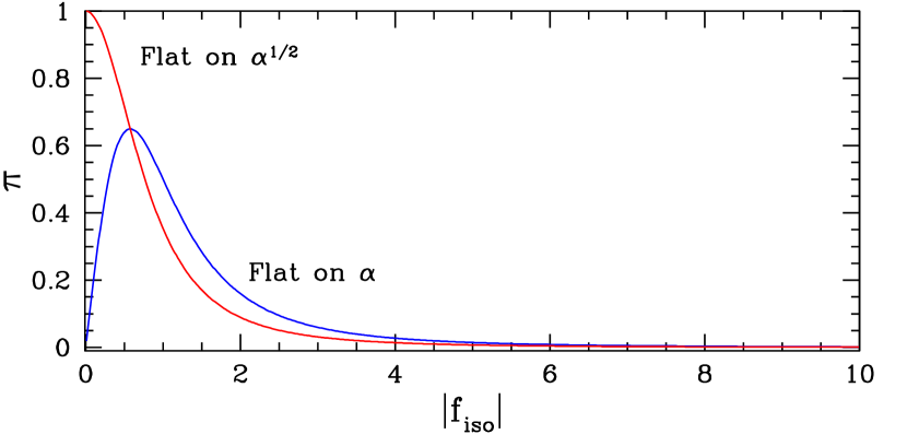
Figure 2: Equivalent priors on $|f_{\text{iso}}|$ corresponding to the flat priors used in Beltran et al. (2005) for the parameters $\alpha$ and $\sqrt{\alpha}$. Both priors cut away the parameter space $|f_{\text{iso}}|\gg 1$, thus reducing the Occam’s razor effect caused by a scale-free parameter. The odds in favor of the purely adiabatic model thus become correspondingly smaller. Model comparison results can depend crucially on the variables adopted.

This example illustrates that model comparison results can depend crucially on the underlying parameter space. We now turn to discuss the dependence of our other results on the prior range one chooses to adopt.

3.3 Dependence on the choice of prior

As described in detail in Appendix A, the Bayes factor is really a function of two parameters, $\lambda$ and the information content $I=-\ln\beta$, see Eq. (21) for the case of a Gaussian prior and a Gaussian likelihood in the parameter of interest. Figure 3 shows contours of $|\ln B_{01}|=\text{const}$ for $\text{const}=1.0,2.5,5.0$ in the $(I,\lambda)$ plane, as computed from Eq. (21). The contours delimit significative levels for the strength of evidence, as summarized in Table 1. In the following, we will measure the information content $I$ in base–10 logarithm. For moderately informative data ($I\approx 1-2$) the measured mean has to lie at least about $4\sigma$ away from $\omega_{\star}$ in order to robustly disfavor the simpler model (i.e., $\lambda\,\raise 1.72218pt\hbox{$>$}\kern-6.99997pt\lower 2.6694pt\hbox{$\sim$}\,4$). Conversely, for $\lambda\,\raise 1.72218pt\hbox{$<$}\kern-8.00003pt\lower 2.6694pt\hbox{$\sim$}\,3$ highly informative data ($I\,\raise 1.72218pt\hbox{$>$}\kern-6.99997pt\lower 2.6694pt\hbox{$\sim$}\,2$) do favor the conclusion that $\omega=\omega_{\star}$. In general, a large information content favors the simpler model, because Occam’s razor penalizes the large volume of “wasted” parameter space of the extended model. A large $\lambda$ disfavors exponentially the simpler model, in agreement with the sampling theory result. The location on the plane of the three cases discussed in the text (the scalar spectral index, the spatial curvature and the CDM isocurvature component) is marked by diamonds (circles) for WMAP1+ext (WMAP3+ext). Even though the informative regions of Figure 3 assume a Gaussian likelihood, they are illustrative of the results one might obtain in real cases, and can serve as a rough guide for the Bayes factor determination.

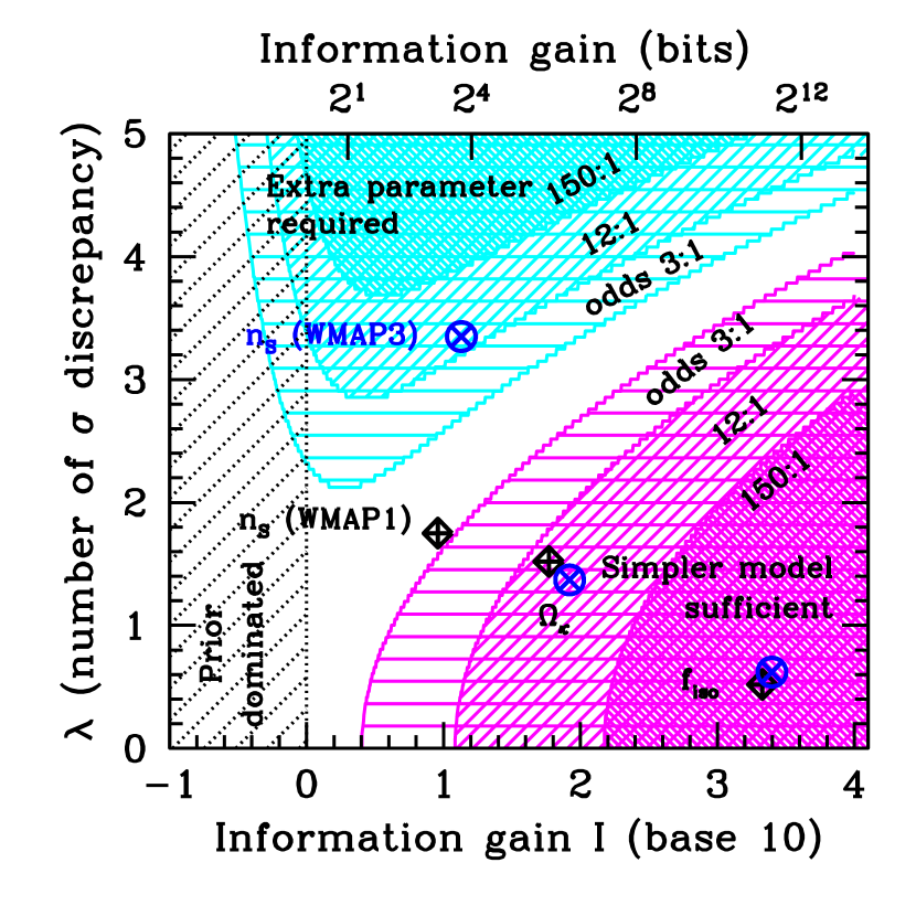
Figure 3: Regions in the $(I,\lambda)$ plane (shaded) where one of the competing models is supported by positive (odds of 3:1), moderate (12:1) or strong (odds larger than 150:1) evidence. The white region corresponds to an inconclusive result (odds of about 1:1), while in the region $I<0$ (dotted) the posterior is dominated by the prior and the measurement is non–informative. In the lower horizontal axis, $I$ is given in base 10, i.e. $I=-\log_{10}\beta$, while it is given in bits in the upper horizontal axis. The contours are computed from the SDDR formula assuming a Gaussian likelihood and a Gaussian prior. The location of the three parameters analyzed in the text is shown by diamonds (circles) for WMAP1+ext data (WMAP3+ext data). Choosing a wider (narrower) prior range would shift the points horizontally to the right (to the left) of the plot.

Another useful properties of displaying the result of the model comparison in the $(I,\lambda)$ plane as in Figure 3 is that the impact of a change of prior can be easily estimated. A different choice of prior will amount to a horizontal shift of the points in Figure 3, at least as long as $I>0$ (i.e., posterior dominated by the likelihood). Thus we can see that given the results with the priors used in this paper, no other choice of priors for $f_{\text{iso}}$ or $\Omega_{\kappa}$ within 4 order of magnitude will achieve a reversal of the conclusion regarding the favoured model. At most, picking more restrictive priors (reflecting more predictive theoretical models) would make the points for $f_{\text{iso}}$ or $\Omega_{\kappa}$ drift to the left of Figure 3, eventually entering in the white, inconclusive region $I\,\raise 1.72218pt\hbox{$<$}\kern-8.00003pt\lower 2.6694pt\hbox{$\sim$}\,0.5$. For the spectral index from WMAP 3–year data, choosing a prior 2 orders of magnitude larger than the one employed here, ie $-19<n_{S}<20$ would reverse the conclusion of the model selection, favouring the model $n_{S}=1$ with odds of about 3:1. This choice of prior is however physically unmotivated. On the other hand, reducing the prior by one order of magnitude – i.e., making it of the same order as the current posterior width ($I=0$) – would still not alter the conclusion that $n_{S}=1$ is disfavoured with moderate odds.

The prior assignment is an irreducible feature of Bayesian model selection, as it is clear from its presence in the denominator of Eq. (7). There is a vast literature which adresses the problem of assigning prior probabilities (see footnote 1) in a way which reflects the state of knowledge before seeing the data. In applications to model selection, it might be more useful to regard the prior as expressing the available parameter space under the model, rather then a state of knowledge before seeing the data, as argued in Kunz et al. (2006). The underpinnings of the prior choice can be found in our understanding of model–specific issues. In this work we have offered two examples of priors stemming from theoretical motivations: the prior on the scalar spectral index is a consequence of assuming slow–roll inflation while the prior on the spatial curvature comes from our knowledge that the Universe is not empty (and therefore the curvature must be smaller than $-1$) nor overclosed (or it would have recollapsed). This simple observations set the correct scale for the prior on $\Omega_{\kappa}$, which is of order unity. On the other hand, if one wanted to impose an inflation–motivated prior of width $\ll 1$, then the information content of the data would go to 0 and the outcome of the model selection would be non-informative. In general, it is enough to have an order of magnitude estimate of the a priori allowed range for the parameter of interest, since the logarithm of the model likelihood is proportional to the logarithm of the prior range. Furthermore, considerations of the type outlined above can help assessing the impact of a prior change on the model comparison outcome. Often one will find that most “reasonable” prior choices will lead to qualitatively to the same conclusion, or else to a non–committal result of the model comparison.

For essentially scale–free parameters, such as the adiabatic and isocurvature amplitudes of our third application, model theoretical considerations of the type employed by Lazarides et al. (2004) can lead to a limitation of the prior range. In the context of phenomenological model building, we have demonstrated that an analysis of the a priori parameter space accessible to the instrument can be used to define a prior encapsulating our expectations on the quality of the data we will be able to gather.

An important caveat is the dependence of the Bayes factor on the basis one adopts in parameter space, which sets the natural measure on the parameters. A flat prior on ${\theta}$ does not correspond to a flat prior on some other set $\alpha({\theta})$ obtained via a non–linear transformation, since the two prior distributions are related via

$$\pi({\theta}|{M})=\pi({\alpha}|{M})\Big{|}\frac{\textrm{d}{\alpha}({\theta})}{\textrm{d}{\theta}}\Big{|}.$$ (12)

As illustrated by the case of the isocurvature amplitude, this is especially relevant for parameters which can vary over many orders of magnitudes. We put forward that the choice of the parameter basis can be guided by our physical insight of the model under scrutiny and our understanding of the observations. This principle would suggest that one should adopt flat priors along “normal variables” or principal components, because those are directly probed by the data and usually can be interpreted in terms of physically relevant and meaningful quantities. A general principle of consistency can be invoked to select the most appropriate variable for cases where many apparently equivalent choices are present (for example, $f_{\text{iso}}$, $\alpha$ or $\sqrt{\alpha}$). We leave further exploration of this very relevant issue to a future publication.

4 Conclusions

We have argued that frequentist significance tests should be interpreted carefully and in particular that Bayesian model selection reasoning should be used to decide whether the introduction of a parameter is warranted by data. The main strengths of the Bayesian approach are that it does consider the information content of the data and that it allows one to confirm predictions of a model, instead of just disproving them as in the sampling theory approach.

We have investigated the use of the Savage–Dickey density ratio (SDDR) as a tool to compute the Bayes factor of two nested models, at no extra computational cost than the Monte Carlo sampling of the parameter space. The technique is likely to be accurate for cases where the the estimated value of the extra parameter under the larger model lies less than about 3 sigma’s away from the predicted value under the simpler model, as shown in Appendix C. In a companion paper (Trotta, 2007a) a complementary technique is introduced, called PPOD, which produces forecasts for the probability distribution of the Bayes factor from future experiments.

We have applied this Bayesian model selection point of view to three central ingredients of present–day cosmological model building. Regarding the spectral index of scalar perturbations, we found that WMAP 3–year data disfavour a scale–invariant spectral index with moderate evidence, and that this result holds true for all reasonable choices of priors. This is a significant change with respect to the inconclusive result one obtained using the WMAP 1st year data release instead. We found that the odds in favour of a flat Universe have doubled (from $15:1$ to $29:1$) in going from WMAP1+ext to WMAP3+ext, and we have stressed that this conclusion can only be obtained if the Hubble parameter is measured independently or if supernovae luminosity distance measurements (or other low–redshift rulers, such as baryonic acoustic oscillations, see Eisenstein et al. (2005)) are employed. Finally, purely adiabatic initial conditions are strongly preferred to a mixed model containing a totally (anti)correlated CDM isocurvature contribution (odds larger than $1000:1$), on the grounds of an Occam’s razor argument, that the prior available parameter space is much larger than the small surviving posterior volume. This is however crucially dependent on the variable one chooses to impose flat priors on.

In the light of these findings, it seems to us that model comparison tools offer complementary insight in what the data can tell us about the plausibility of theoretical speculations regarding cosmological parameters, and can provide useful guidance in the quest of a cosmological concordance model.

Acknowledgments I am grateful to Chiara Caprini, Ruth Durrer, Samuel Leach, Julien Lesgourgues and Christophe Ringeval for useful discussions. I thank Martin Kunz, Andrew Liddle, Tom Loredo, Pia Mukherjee and David Parkison for many enlightening discussions and valuable comments on earlier drafts. I thank an anonymous referee for many helpful suggestions. This research is supported by the Tomalla Foundation, by the Royal Astronomical Society through the Sir Norman Lockyer Fellowship and by St Anne’s College, Oxford. The use of the Myrinet cluster (University of Geneva) and of the Glamdring cluster (Oxford University) is acknowledged. I acknowledge the use of the package cosmomc, available from cosmologist.info, and the use of the Legacy Archive for Microwave Background Data Analysis (LAMBDA). Support for LAMBDA is provided by the NASA Office of Space Science.

Appendix A An illustration of Lindley’s paradox

Lindley (1957)’s paradox describes a situation where frequentist significance tests and Bayesian model selection procedures give contradictory results. As we demonstrate below, it arises because the information content of the data is neglected in the frequentist approach.

Let us consider the toy example of a measurement of a Gaussian distributed quantity, $\omega$, by drawing $n$ iid samples with known s.d. $\sigma$. Then the likelihood function is the normal distribution

$$p(\hat{\mu},\hat{\sigma}|\omega)={N_{\hat{\mu},\hat{\sigma}}(\omega)},$$ (13)

where $\hat{\mu}$ is the estimated mean and $\hat{\sigma}=\sigma/\sqrt{n}$ its uncertainty. From the point of view of frequentist statistics, a significance test is performed on the null hypothesis $\mathcal{H}_{0}:\omega=\omega_{\star}$. We define $\lambda$ as dimensionless number which indicates “how many sigma’s away” is our estimate of the mean, $\hat{\mu}$, from its value under $\mathcal{H}_{0}$ in units of its uncertainty:

$$\lambda\equiv\frac{|\hat{\mu}-\omega_{\star}|}{\hat{\sigma}}.$$ (14)

This “number of sigma’s” difference is interpreted as a measure of the confidence with which one can reject $\mathcal{H}_{0}$. The “p–value”

$$\text{p--value}=\int_{\lambda}^{\infty}p(\hat{\mu},\hat{\sigma}|\omega)\textrm{d}\omega$$ (15)

is compared to a number $\alpha$, called the “significance level” of the test and the hypothesis $\mathcal{H}_{0}$ is rejected at the $1-\alpha$ confidence level if $\text{p--value}<\alpha$. If we pick a (fixed) confidence level, say $\alpha=0.05$, then the frequentist significance test rejects the null hypothesis if

$$Z(\lambda)\equiv\frac{1}{\sqrt{2\pi}}\int_{\lambda}^{\infty}\exp\left(-t^{2}/2\right)\textrm{d}t\leq\alpha/2.$$ (16)

(for a 2–tailed test). For $\alpha=0.05$ the equality in Eq. (16) holds for $\lambda=1.96$. In other words, sampling statistics reject the null hypothesis at the 95% confidence level if the measured mean is more than $\lambda=1.96$ sigma’s away from the predicted $\omega_{\star}$ under $\mathcal{H}_{0}$.

This conclusion can be in strong disagreement with the Bayesian evaluation of the Bayes factor, i.e. a value $\omega_{\star}$ rejected under a frequentist test can on the contrary be favored by Bayesian model comparison (Lindley, 1957). In the Bayesian model comparison approach, the two competing models are ${M}_{0}$, with no free parameters, in which the value of $\omega$ is fixed to $\omega=\omega_{\star}$, and model ${M}_{1}$, with one free parameter $\omega\neq\omega_{\star}$. Under ${M}_{1}$, our prior belief before seeing the data on the probability distribution of $\omega$ is explicitly represented by the prior pdf $\pi(\omega)$. This prior pdf is then updated to the posterior via Bayes theorem, Eq. (1).

A formal measure of the information gain obtained through the data is the cross–entropy between prior and posterior, the Kullback–Leibler divergence

$$D_{KL}(p,\pi)=\int p({\theta}|{d})\ln\frac{p({\theta}|{d})}{\pi({\theta})}\textrm{d}{\theta}.$$ (17)

For a Gaussian prior of standard deviation $\Delta\omega$ centered on $\omega_{\star}$ and a Gaussian likelihood with mean $\hat{\mu}$ and standard deviation $\hat{\sigma}$, the information gain is given by

$$D_{KL}+\frac{1}{2}=-\ln\beta+\frac{1}{2}\beta^{2}(\lambda^{2}-1),$$ (18)

where we have defined

$$\beta\equiv\hat{\sigma}/\Delta\omega,$$ (19)

the factor by which the accessible parameter space under ${M}_{1}$ is reduced after the arrival of the data (remember that $\hat{\sigma}$ is the standard deviation of the likelihood). For totally uninformative data, $\beta=1$ and $\lambda=0$, and thus $D_{KL}=0$. Unless $\lambda\gg 1$ (in which case the null hypothesis is rejected with many sigma’s and there is hardly any need for model comparison) we can usually neglect the second term on the right–hand–side of Eq. (18). We are therefore led to define a simpler measure of the information content of the data, $I$, as

$$I\equiv-\ln\beta.$$ (20)

The choice of the logarithm base is only a matter of convenience, and this sets the units in which the entropy is measured. Had we chosen base–2 logarithm instead, the information would have been measured in bits. In Figure 3, the choice of using the base–10 logarithm for the bottom horizontal axis means that $I$ describes the order of magnitude by which our prior knowledge has improved after the arrival of the data.

We now compute the Bayes factor $B_{01}$ in favor of model ${M}_{0}$ from Eq. (7), using again the above Gaussian prior, obtaining

$$B_{01}(\beta,\lambda)=\sqrt{1+\beta^{-2}}\exp\left(-\frac{\lambda^{2}}{2(1+\beta^{2})}\right).$$ (21)

The model comparison result thus depends not only on $\lambda$, but also on the quantity $\beta$, which is proportional to the volume occupied by the posterior in parameter space and describes the information gain in going from prior to posterior. If instead of a Gaussian prior one takes a flat prior around $\omega_{\star}$ of width $2\Delta\omega$ (the factor of 2 being chosen to facilitate the comparison with the case of a Gaussian prior of standard deviation $\Delta\omega$) one obtains instead

$$B_{01}(\beta,\lambda) =\sqrt{\frac{2}{\pi}}\beta^{-1}\exp\left(-\lambda^{2}/2\right)\times$$ (22)

$$\left[Z\left(\lambda-\beta^{-1}\right)-Z\left(\lambda+\beta^{-1}\right)\right]^{-1}.$$

where the function $Z(y)$ is defined in (16), a consequence of the top–hat prior. For $\beta^{-1}\gg\lambda$, the posterior is well localized within the boundaries of the prior and the term in square brackets in (22) tends to $1$.

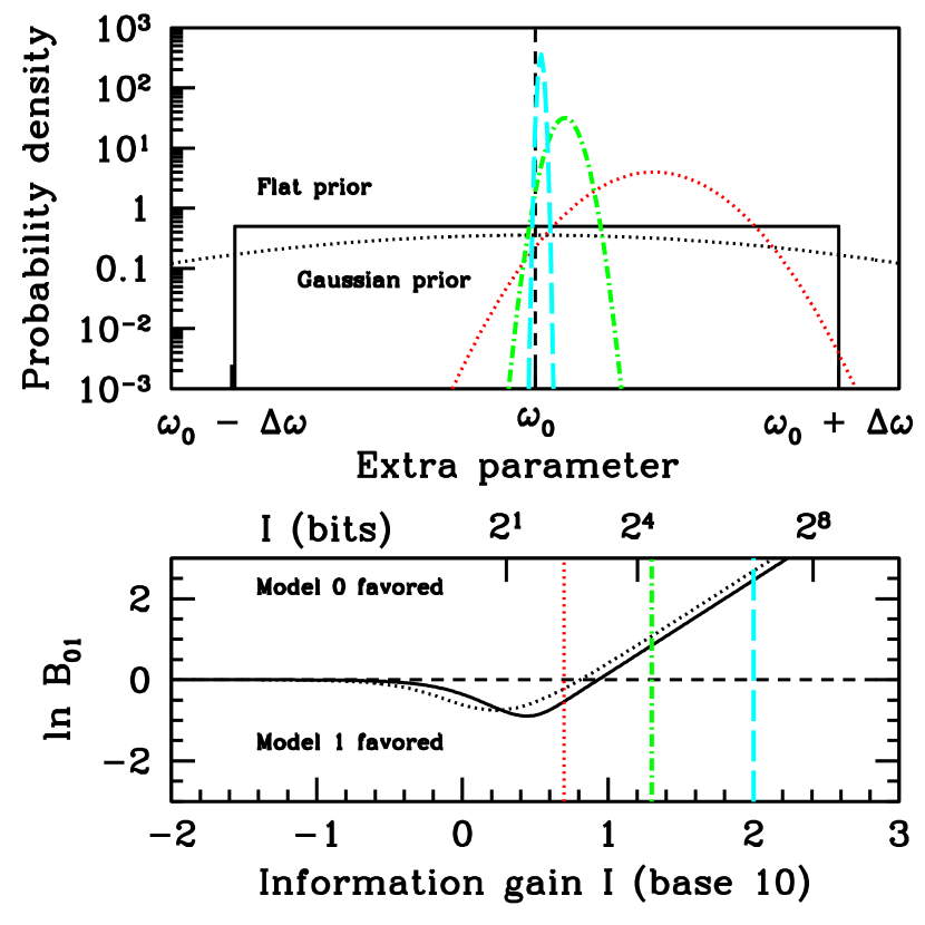
Figure 4: Illustration of Lindley’s paradox. Sampling statistics hypothesis testing rejects the hypothesis that $\omega=\omega_{\star}$ with 95% confidence in all 3 cases (coloured curves) illustrated in the top panel ($\lambda=1.96$ in all cases). Bayesian model selection does take into account the information content of the data $I$, and correctly favors the simpler model (predicting that $\omega=\omega_{\star}$) for informative data (right vertical line in the bottom panel, $I=2$ expressed in base–10 logarithm), with odds of $14:1$ (for a Gaussain prior, dotted black line). Using a flat prior of the same width (solid black line) instead reduces $\ln B_{01}$ by a geometric factor $\ln(2/\pi)/2=0.22$ in the informative ($I\gg 1$) regime. Notice that for non–informative data ($I\ll 0$) the Bayes factor reverts to equal odds for the two models.

In order to clarify the role of the information content and the difference with frequentist hypothesis testing, consider the following example (see Figure 4). For a fixed choice of prior width $\Delta\omega$, imagine performing three different measurements, each with a different value of $\beta$ (i.e., with different information content $I$) but with outcomes such that $\lambda$ is the same in all three cases. This is depicted in the top panel of Figure 4, where the likelihood mean is $\lambda=1.96$ sigma’s away from $\omega_{\star}$ for all three cases. Under sampling statistics, all three measurements equally reject the null hypothesis, that $\omega=\omega_{\star}$, at the 95% confidence level. And yet common sense clearly tells us that this cannot be the right conclusion in all three cases. Indeed, the Bayes factor, Eq. (21) or (22), correctly recovers the intuitive result (bottom panel of Figure 4): the measurement with the larger error ($\beta=1/5$, or $I=0.7$, expressed in base–10 logarithm) corresponds to the least informative data, and the Bayes factor slightly disfavours the simpler model ($\ln B_{01}=-0.2$, or odds of about 5:4 against ${M}_{0}$ and $p({M}_{0}|{d})=0.44$). For $\beta=1/20$ or $I=1.3$ (moderately informative data), evidence starts to accumulate in favor of ${M}_{0}$ ($\ln B_{01}=1.08$, odds of 3:1 in favor and $p({M}_{0}|{d})=0.75$). For very informative data, $\beta=1/100,I=2$, Bayesian reasoning correctly deduces that the simpler ${M}_{0}$ should be favored ($\ln B_{01}=2.68$, odds of 14:1 in favor of ${M}_{0}$ and a posterior probability $p({M}_{0}|{d})=0.94$). The above numbers are for a Gaussian prior, but those conclusion are largely independent of the choice of a Gaussian or of a flat prior, provided the bulk of the prior volume is the same (compare the dotted and solid line in the bottom panel of Figure 4 for a Gaussian and a flat prior, respectively).

This illustration shows that the Bayes factor can correctly favor models which would be rejected with high confidence by hypothesis testing in a sampling theory approach. While in sampling theory one is only able to disprove models by rejecting hypothesis, it is important to highlight that the Bayesian evidence can and does accumulate in favor of simpler models, scaling as $1/\beta$. While it is easier to disprove $\omega=\omega_{\star}$, since model rejection is exponential with $\lambda$, the Bayesian approach allows to evaluate what the data have to say in favor of an hypothesis, as well.

In summary, quoting the number of sigma’s away from $\omega_{\star}$ (the $\lambda$ parameter) is not always an informative statement to decide whether or not a parameter $\omega$ differs from $\omega_{\star}$. Answering this question is a model comparison issue, which requires the evaluation of the Bayes factor.

Appendix B Derivation of the SDDR

The Bayes factor $B_{01}$ of Eq. (2) can be evaluated by computing the integrals

$$p({M}_{0}|{d}) =\int\textrm{d}\psi\pi_{0}(\psi)p({d}|\psi,\omega_{\star}),$$ (23)

$$p({M}_{1}|{d}) =\int\textrm{d}\psi\textrm{d}\omega\pi_{1}(\psi,\omega)p({d}|\psi,\omega)\equiv q.$$ (24)

Here $\pi_{0}(\psi)$ denotes the prior over $\psi$ in model ${M}_{0}$, and $\pi_{1}(\psi,\omega)$ the prior over $(\psi,\omega)$ under model ${M}_{1}$. Note that, since the models are nested, the likelihood function for ${M}_{0}$ is just a slice at constant $\omega=\omega_{\star}$ of the likelihood function in model ${M}_{1}$, $p({d}|\psi,\omega)$.

Now multiply and divide $B_{01}$ by the number $p(\omega_{\star}|{d})\equiv p(\omega=\omega_{\star}|{d},{M}_{1})$, which is the marginalized posterior for $\omega$ under ${M}_{1}$ evaluated at $\omega_{\star}$, and using that $p(\omega_{\star}|{d})=p(\omega_{\star},\psi|{d})/p(\psi|\omega_{\star},{d})$ at all points $\psi$, we obtain

$$B_{01} =p(\omega_{\star}|{d})\int\textrm{d}\psi\frac{\pi_{0}(\psi)p({d}|\psi,\omega_{\star})p(\psi|\omega_{\star},{d})}{q\cdot p(\omega_{\star},\psi|{d})}$$ (25)

$$=p(\omega_{\star}|{d})\int\textrm{d}\psi\frac{\pi_{0}(\psi)p(\psi|\omega_{\star},{d})}{\pi_{1}(\omega_{\star},\psi)},$$ (26)

where in the second equality we have used the definition of posterior, namely that $p(\omega_{\star},\psi|{d})=p({d}|\omega_{\star},\psi)\pi_{1}(\omega_{\star},\psi)/q$. Up to this point we have not made any assumption nor approximation. We now assume that the prior satisfies

$$\pi_{1}(\psi|\omega_{\star})=\pi_{0}(\psi),$$ (27)

which always holds in the (usual in cosmology) case of separable priors, i.e.

$$\pi_{1}(\omega,\psi)=\pi_{1}(\omega)\pi_{0}(\psi).$$ (28)

Under this assumption, and since $p(\psi|\omega_{\star},{d})$ in (26) is the normalized marginal posterior, Eq. (26) simplifies to the SDDR given in Eq. (7).

Appendix C Benchmark tests for the SDDR

In order to explore the accuracy of the SDDR, we have tested its performance for the benchmark case of a Gaussian likelihood. A $D$–dimensional likelihood is generated by choosing a random $D$–dimensional, diagonal covariance matrix. The correlations can be set to 0 without loss of generality since in the Gaussian case it is always possible to rotate to the principal axis of the covariance ellipse. The mean of the likelihood is set to 0 for the last $D-1$ dimensions, while for the first parameter (the one we are interested in testing) the mean is chosen to lie $\lambda\sigma_{1}$ away from 0, where $\lambda$ is selected below and $\sigma_{1}^{2}$ is the covariance along direction 1. We then compare the two following nested models: ${M}_{0}$ predicts that the first parameter $\theta_{1}=0$, while ${M}_{1}$ has a Gaussian prior centered around 0 and of width $\Delta w=\sigma_{1}/\beta$, where $\beta$ is fixed.

The posterior is then reconstructed using a MCMC algorithm and the Bayes factor computed using the SDDR. The results are shown in Figure 5 as a function of the number of samples for parameter spaces of dimension $D=5,10,20$ and for $\lambda=1,2,3$. We have fixed $\beta=0.2$ throughout (changing the value of $\beta$ only rescales the Bayes factor without affecting the accuracy, as long as $\beta<1$, i.e. for informative data). The errors on the Bayes factor are computed as in the text using a bootstrap technique: the full sample set is divided in $R=5$ subsets, then the mean and standard deviation of the SDDR are computed from those subsets. The error thus only reflect the statistical noise within the chain and it does not take into account a possible systematic under–exploration of the likelihood’s tails.

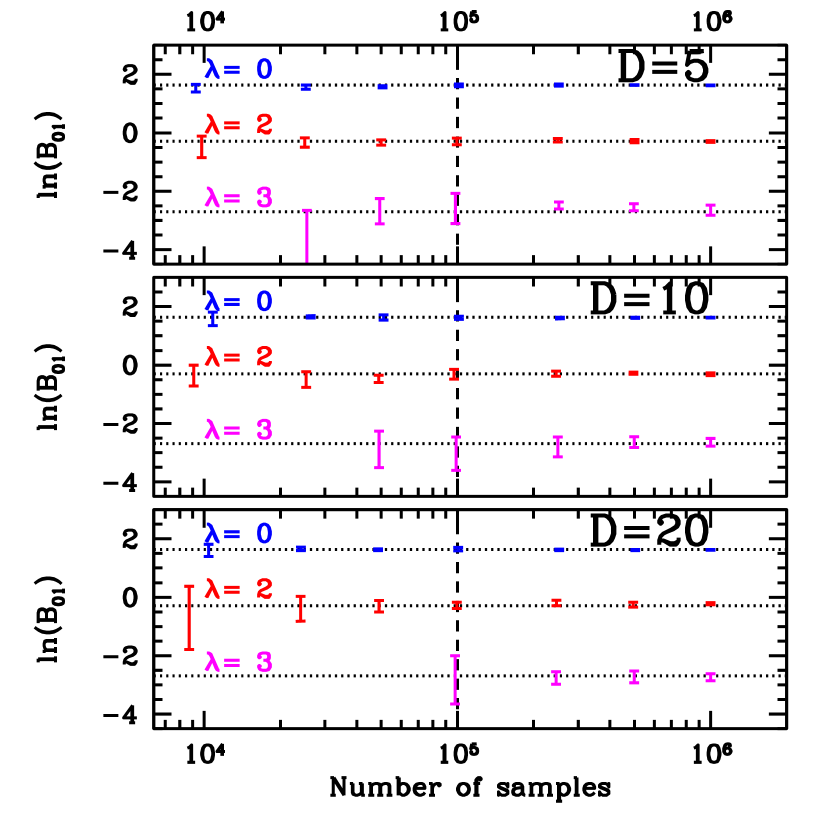
Figure 5: Benchmark test for the SDDR formula for a Gaussian likelihood and prior, for parameter spaces of dimensionality $D$. The horizontal, dotted lines give the exact value. The SDDR performs extremely well for comparing models lying $\lambda<3$ sigma’s away from each other. In this case, less than $10^{5}$ samples are required to achieve a satisfactory agreement with the exact result. For $\lambda\,\raise 1.72218pt\hbox{$>$}\kern-6.99997pt\lower 2.6694pt\hbox{$\sim$}\,4$ the tails of the likelihood are not sufficiently explored to apply the SDDR. The missing points for $\lambda=3$ indicate that the given number of samples are insufficient to achieve coverage of the simpler model prediction.

It is clear that the SDDR performs extremely well for $\lambda\leq 2$ while it becomes less accurate for $\lambda=3$. This is because it is rather difficult to explore regions further out in the tails of the distribution using conventional MCMC methods. For $\lambda>3$ it becomes very unpractical to obtain sufficient samples in the tail. For models that lie less than about 3 sigma’s away from each other, the SDDR gives a satisfactory accuracy in the model comparison result at no extra cost than the parameter estimation step, requiring less than $10^{5}$ samples. Furthermore, the scaling with the dimensionality of the parameter space appears to be rather favourable, and the error increases only mildly from $D=5$ to $D=20$ at a given number of samples.

Clearly, for likelihoods that are close to Gaussian, the approximations (21) and (22) can still give a useful order of magnitude estimate of the result. Finally, we stress that in the regime where the SDDR works well ($\lambda\,\raise 1.72218pt\hbox{$<$}\kern-8.00003pt\lower 2.6694pt\hbox{$\sim$}\,3$) its accuracy is not limited by the assumption of normality of the likelihood, but only by the efficiency and accuracy of the MCMC reconstruction of the posterior. Particular care must be exercised in exploring accurately distributions presenting heavier tails than Gaussians, and further work is required to extend the MCMC sampling to the regime $\lambda\,\raise 1.72218pt\hbox{$>$}\kern-6.99997pt\lower 2.6694pt\hbox{$\sim$}\,4$. In this case, sampling at a higher temperature could help in obtaining sufficient samples in the tail, an issue whose exploration we leave for future work.

References

- Amendola et al. (2002) Amendola L., Gordon C., Wands D., Sasaki M., 2002, Phys. Rev. Lett., 88, 211302
- Bassett et al. (2004) Bassett B. A., Corasaniti P. S., Kunz M., 2004, Astrophys. J., 617, L1
- Bean et al. (2006) Bean R., Dunkley J., Pierpaoli E., 2006, Phys. Rev., D74, 063503
- Beltran et al. (2005) Beltran M., Garcia-Bellido J., Lesgourgues J., Liddle A. R., Slosar A., 2005, Phys. Rev., D71, 063532
- Beltran et al. (2004) Beltran M., Garcia-Bellido J., Lesgourgues J., Riazuelo A., 2004, Phys. Rev., D70, 103530
- Bennett et al. (2003) Bennett C. L., et al., 2003, Astrophys. J. Suppl., 148, 1
- Bowen et al. (2002) Bowen R., Hansen S. H., Melchiorri A., Silk J., Trotta R., 2002, Mon. Not. Roy. Astron. Soc., 334, 760
- Bucher et al. (2004) Bucher M., Dunkley J., Ferreira P. G., Moodley K., Skordis C., 2004, Phys. Rev. Lett., 93, 081301
- Crotty et al. (2003) Crotty P., Garcia-Bellido J., Lesgourgues J., Riazuelo A., 2003, Phys. Rev. Lett., 91, 171301
- DiCiccio et al. (1997) DiCiccio T., Kass R., Raftery A., Wasserman L., 1997, J. Amer. Stat. Assoc., 92, 903
- Dickey (1971) Dickey J. M., 1971, Ann. Math. Stat., 42, 204
- Drell et al. (2000) Drell P. S., Loredo T. J., Wasserman I., 2000, Astrophys. J., 530, 593
- Eisenstein et al. (2005) Eisenstein D. J., et al., 2005, Astrophys. J., 633, 560
- Freedman et al. (2001) Freedman W. L., et al., 2001, Astrophys. J., 553, 47
- Gordon & Lewis (2003) Gordon C., Lewis A., 2003, Phys. Rev., D67, 123513
- Hinshaw et al. (2003) Hinshaw G., et al., 2003, Astrophys. J. Suppl., 148, 135
- Hinshaw et al. (2006) Hinshaw G., et al., 2006, astro-ph/0603451
- Hobson et al. (2002) Hobson M. P., Bridle S. L., Lahav O., 2002, Mon. Not. Roy. Astron. Soc., 335, 377
- Hobson & McLachlan (2003) Hobson M. P., McLachlan C., 2003, Mon. Not. Roy. Astron. Soc., 338, 765
- Jaffe (1996) Jaffe A. H., 1996, Astrophys. J., 471, 24
- Jaynes (2003) Jaynes E., 2003, Probability Theory. The logic of science. Cambridge University Press, Cambridge, U.K.
- Jeffreys (1961) Jeffreys H., 1961, Theory of probability, 3rd edn. OUP
- Kass & Raftery (1995) Kass R., Raftery A., 1995, J. Amer. Stat. Assoc., 90, 773
- Keskitalo et al. (2006) Keskitalo R., Kurki-Suonio H., Muhonen V., Valiviita J., 2006, astro-ph/0611917
- Kosowsky et al. (2002) Kosowsky A., Milosavljevic M., Jimenez R., 2002, Phys. Rev., D66, 063007
- Kunz et al. (2006) Kunz M., Trotta R., Parkinson D., 2006, Phys. Rev., D74, 023503
- Kuo et al. (2004) Kuo C.-l., et al., 2004, Astrophys. J., 600, 32
- Kurki-Suonio et al. (2005) Kurki-Suonio H., Muhonen V., Valiviita J., 2005, Phys. Rev., D71, 063005
- Lazarides et al. (2004) Lazarides G., de Austri R. R., Trotta R., 2004, Phys. Rev., D70, 123527
- Lesgourgues & Pastor (2006) Lesgourgues J., Pastor S., 2006, Phys. Rept., 429, 307
- Lewis & Bridle (2002) Lewis A., Bridle S., 2002, Phys. Rev., D66, 103511
- Lindley (1957) Lindley D., 1957, Biometrika, 44, 187
- Loredo & Lamb (2002) Loredo T. J., Lamb D. Q., 2002, Phys. Rev., D65, 063002
- Lyth & Wands (2003) Lyth D. H., Wands D., 2003, Phys. Rev., D68, 103516
- MacKay (2003) MacKay D., 2003, Information theory, inference, and learning algorithms. Cambridge University Press, Cambridge, U.K.
- Marshall et al. (2006) Marshall P., Rajguru N., Slosar A., 2006, Phys. Rev., D73, 067302
- Moodley et al. (2004) Moodley K., Bucher M., Dunkley J., Ferreira P. G., Skordis C., 2004, Phys. Rev., D70, 103520
- Mukherjee et al. (2006) Mukherjee P., Parkinson D., Liddle A. R., 2006, Astrophys. J., 638, L51
- Page et al. (2006) Page L., et al., 2006, astro-ph/0603450
- Parkinson et al. (2006) Parkinson D., Mukherjee P., Liddle A. R., 2006, Phys. Rev., D73, 123523
- Pierpaoli et al. (1999) Pierpaoli E., Garcia-Bellido J., Borgani S., 1999, JHEP, 10, 015
- Readhead et al. (2004) Readhead A. C. S., et al., 2004, Astrophys. J., 609, 498
- Riess et al. (2004) Riess A. G., et al., 2004, Astrophys. J., 607, 665
- Saini et al. (2004) Saini T. D., Weller J., Bridle S. L., 2004, Mon. Not. Roy. Astron. Soc., 348, 603
- Skilling (2004) Skilling J., 2004, Nested sampling for general Bayesian computation, available from: http://www.inference.phy.cam.ac.uk/bayesys
- Slosar et al. (2003) Slosar A., et al., 2003, Mon. Not. Roy. Astron. Soc., 341, L29
- Spergel et al. (2006) Spergel D. N., et al., 2006, astro-ph/0603449
- Tegmark et al. (2004) Tegmark M., et al., 2004, Astrophys. J., 606, 702
- Trotta (2004) Trotta R., 2004, PhD Thesis N. 3534, University of Geneva, Switzerland, June 2004
- Trotta (2005) Trotta R., 2005, Available as v1 from astro-ph/0504022-v1
- Trotta (2007a) Trotta R., 2007a, Mon. Not. R. Astron. Soc. in press, astro-ph/0703063
- Trotta (2007b) Trotta R., 2007b, Mon. Not. R. Astron. Soc., 375, L26, astro-ph/0608116
- Trotta (2007c) Trotta R., 2007c, New Astron. Rev., 51, 316, astro-ph/0607496
- Trotta & Durrer (2006) Trotta R., Durrer R., In M. Novello and S. Perez Bergliaffa, eds, Proceedings of the MG10 Meeting held at Brazilian Center for Research in Physics (CBPF) Rio de Janeiro, Brazil 20 – 26 July 2003. World Scientific (2006).
- Trotta & Hansen (2004) Trotta R., Hansen S. H., 2004, Phys. Rev., D69, 023509
- Trotta et al. (2001) Trotta R., Riazuelo A., Durrer R., 2001, Phys. Rev. Lett., 87, 231301
- Trotta et al. (2003) Trotta R., Riazuelo A., Durrer R., 2003, Phys. Rev., D67, 063520
- Valiviita & Muhonen (2003) Valiviita J., Muhonen V., 2003, Phys. Rev. Lett., 91, 131302
- Verde et al. (2003) Verde L., et al., 2003, Astrophys. J. Suppl., 148, 195
- Verdinelli & Wasserman (1995) Verdinelli I., Wasserman L., 1995, J. Amer. Stat. Assoc., 90, 614