Modified Newtonian Dynamics In Dimensionless Form

Abstract

Modified Newtonian dynamics proposed that gravitational field needs modifications when the field strength $g$ is weaker than a critical value $g_{0}$. This has been shown to be a good candidate as an alternative to cosmic dark matter. There is another way to look at this theory as a length scale dependent theory. One will show that modification of the Newtonian field strength depends on the mass distribution and the coordinate scale of the system. It is useful to separate the effective gravitation field $g(r)$ into a small scale (or short-distance )$g_{s}$ field and a large scale (or a long-distance) $g_{l}$ field that should be helpful for a better understanding of the underlying physics. The effective potential is also derived.

I INTRODUCTION

Modified Newtonian dynamics (MOND) was proposed by Milgrom (1983) that gravitational field needs modifications when the field strength $g$ is weaker than a critical value $g_{0}$. This has been shown to be a good candidate as an alternative to cosmic dark matter (Sanders 2001). The phenomenological foundations for MOND are based on two observational facts: (1) flat asymptotic rotation curve, (2) the successful Tully-Fisher (TF) law, $M\sim V^{\alpha}$ (Tully & Fisher 1977) for the relation between rotation velocity and luminosity in spiral galaxies. Here $\alpha$ is close to 4.

In this paper, one proposes a different view of MOND by looking at the physics related by the mass distribution and the coordinate scale of the system. In addition, one finds it useful to separate the effective gravitation field $g(r)$ into a small scale (or short-distance )$g_{s}$ field and a large scale (or a long-distance) $g_{l}$ field that should be helpful for a better understanding of the underlying physics. The effective potential is obtained. Possible relation with the induced gravity model is also discussed.

If dark matter does not exit, rotation curve observations indicate that $g$ behaves as $1/r$, a typical $2$-dimensional attraction field, at large distance greater than the galactic scale around $10^{5}$ lightyears. At short distance, $g$ goes like $1/r^{2}$, a typical behavior of a $3$-dimensional attraction field. Therefore, it is also very interesting to study the changing pattern of the effective dimension $d(r)$ which will be defined as a function of the physical scale $r$. One will plot this $d(r)$ functions hoping for a better understanding of the changing pattern of the effective dimension. Possible speculation with the Kaluza-Klein theory will be discussed in this paper too.

We will start by showing how to simplify the expression of MOND field strength by writing it with suitable scale parameters. Our aim is to write all physical quantities in dimensionless form with suitable physical units.

First of all, it was pointed out (Milgrom 1983) that there exists a critical acceleration parameter $g_{0}=1.2\times 10^{-8}{\rm cms}^{-2}$ characterizing the turning point of the effective power law associated with the gravitational field in MOND. Gravitational field of the following form was suggested

$$g\cdot\mu({g\over g_{0}})=g_{N}$$ (1)

with a function $\mu$ considered as a modified inertial. Here $g_{N}$ is the Newtonian gravitational field produced by certain mass distribution. Milgrom argues that

$$\mu(x)={x\over\sqrt{1+x^{2}}}$$ (2)

provides a best fit with many existing observation data including the rotational curve of many spiral galaxies. Observations are selected mostly from the most reliable $21$ cm hydrogen line measurements. The 21 cm hydrogen line is the photon emission due to the superfine energy difference resulting from the magnetic dipole-dipole interactions between the cored proton and orbiting electron. The existing neutron hydrogen all around the invisible region of spiral galaxies provides better estimates on the rotation curves beyond the visible region of spiral galaxies.

Milgrom also points out that the critical parameter $g_{0}$ is close to the value of $cH_{0}\sim 5\times 10^{-8}cms^{-2}$. It is also the gravitational field produced by an $m=200MeV$ massive particle at its Compton surface. Indeed, one finds that $g_{200MeV}=Gm/\lambda=Gm^{3}c^{2}/h^{2}\sim 1.2\times 10^{-8}cms^{-2}$. Milgrom hence speculates that MOND could have to do with the quantum theory of the universe.

Milgrom’s original idea is that the gravitational field needs modification when $g$ is weaker than critical field strength $g_{0}$. It is interesting to find that $r_{0}\sim 49700ly$ if we define the scale length $r_{0}$ via the following equation

$$g_{0}\equiv{GM_{0}\over r_{0}^{2}}$$ (3)

with $M_{0}\equiv 2\times 10^{11}M_{s}$ and $M_{s}$ the solar mass. Note that one takes $M_{0}$ close to the order of magnitude of a typical galaxy similar to our Milky Way. Taking a different value of $M_{0}$ will only change the value of $r_{0}$. Selecting different value of $M_{0}$ and hence $r_{0}$ will not affect our arguments in this paper. One chooses $M_{0}$ and hence the corresponding $r_{0}$ simply to set them as units of scale. Physics will not be affected by the choice of unit.

One observes, however, that $r_{0}$ is pretty close to the radial size of the visible boundary of our Milky Way if $M_{0}$ is chosen close to the total visible mass of Milky Way. This is certainly true as modification is needed only at large scale according to MOND. Starting next section, one will try to write the modified field strength $g$ in a dimensionless form with the help of the parameters $M_{0}$, $r_{0}$ and $g_{0}$. The idea is to write $M$, $r$ and $g$ in units of $M_{0}$, $r_{0}$ and $g_{0}$ respectively.

II Modified Newtonian Dynamics

Milgrom argues that one can take the effective inertial $\mu$ as $\mu(x)=x/\sqrt{1+x^{2}}$. Therefore, one obtains

$${(g/g_{0})^{2}\over\sqrt{1+(g/g_{0})^{2}}}=g_{N}/g_{0}$$ (4)

by dividing both sides of the equation [1] by the critical parameter $g_{0}$. One can therefore write above equation as

$${g^{2}\over\sqrt{1+g^{2}}}=g_{N}$$ (5)

with $g$ and $g_{N}$ written in unit of $g_{0}$. This makes $g$ and $g_{N}$ dimensionless from now on.

Throughout this paper, we will focuss on the study of the system with a Newtonian attraction of the form $g_{N}=Gm/r^{2}$. This is the field strength at a radial distance $r$ from a spherical distributed matter with total mass $m$. System with different mass distribution can be obtained straightforwardly. Note that ${Gm/(r^{2}g_{0})}={mr_{0}^{2}/(M_{0}r^{2})}$. Therefore, one can write $g_{N}=m/r^{2}$ if $g_{N}$, $r$ and $m$ are written in unit of $g_{0}$, $r_{0}$ and $M_{0}$ respectively. Therefore, the modified field strength $g$ can be written as

$${g^{2}\over\sqrt{1+g^{2}}}={m\over r^{2}}$$ (6)

One can further suppress the parameter $m$ by defining $r_{c}\equiv r_{0}\sqrt{m}$ and write $r$ as a dimensionless coordinate variable in unit of $r_{c}$ instead of $r_{0}$. As a result, one can write above equation in a very compact form

$${g^{2}\over\sqrt{1+g^{2}}}={1\over r^{2}}$$ (7)

in terms of above dimensionless parameters. To emphasize again, one writes

$${m\over M_{0}} \to m,$$ (8)

$${g\over g_{0}} \to g,$$ (9)

$${r\over r_{c}}={r\over\sqrt{m}r_{0}} \to r$$ (10)

in order to simplify the expression of the modified equation and make $g$, $g_{N}$, and $r$ dimensionless for convenience. It is straightforward to restore all dimension parameters when one needs to evaluate any corresponding physical values.

First of all, Eq. (7) can be solved to write $g(r)$ as a function of $r$:

$$g={\sqrt{1+\sqrt{1+4r^{4}}}\over\sqrt{2}r^{2}}={1\over r}\exp[{\sinh^{-1}(2r^{2})^{-1}\over 2}].$$ (11)

One can plot the functions $g(r)$ and compare it with the functions $1/r$ and $1/r^{2}$ for a better picture of its small scale and large scale behaviors. Indeed, Figure 1 shows the behavior of $g(r),1/r$, and $1/r^{2}$ together for comparison. Because the difference at short distance scale is too small for comparison, one also plot it in logarithmic scale. Figure 2 was plotted as logarithm of these functions to enlarge the small difference among these functions in the short distance region.

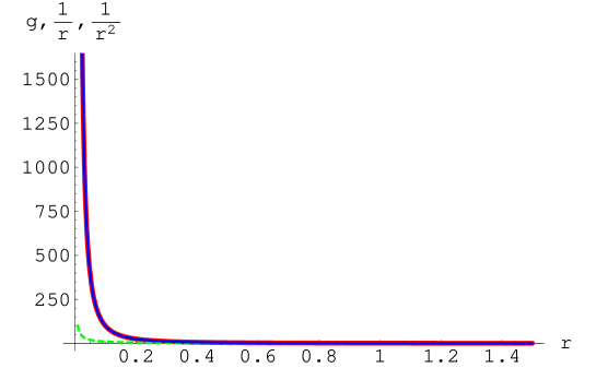
FIG. 1.: $g(r),1/r$ and $1/r^{2}$ plotted as thick solid line, dashed line, and thin solid line respectively. Note that $g$ and $r$ are dimensionless quantities defined in Eq. [8].

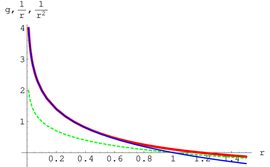
FIG. 2.: Logarithm of $g(r),1/r$ and $1/r^{2}$ plotted as thick solid line, dashed line, and thin solid line respectively. Note that $g$ and $r$ are dimensionless quantities defined in Eq. [8].

It is apparent that $g(r)$ goes like $1/r^{2}$ at short distance scale where $r\ll 1$. On the other hand, $g(r)$ goes like $1/r$ at large distance scale where $r\gg 1$. One can also easily tell from the figures that they agree with our analytic approximation at both the regions $r\ll 1$ and $r\gg 1$ one obtained earlier.

More importantly, writing $g(r)$ as a function of $r\to r/(\sqrt{m}r_{0})$ clearly shows that the Newtonian gravitational field receives significant modification only when $r>1$, or equivalently, $r>r_{c}\equiv\sqrt{m}r_{0}$. This is in fact equivalent to the assumption made by Milgrom that significant modification is required when $g<g_{0}$. The picture looking at the physics related to the physical scale is however easier for a better understanding of possible underlying physics.

Indeed, one easily finds that, if Eq. (11) is the correct gravitational field for all scales, the effective dimension of the system seems to decrease from 3 to 2 as the scale $r$ increases. Geometric dimension seem to decrease if one increase the physical scale of interest. The major difference is that the critical scale depends not only on $r_{0}=\sqrt{GM_{0}/g_{0}}$ but also proportional to $\sqrt{m}$, the square-root of the total mass of the system. One recalls that Kaluza-Klein theory proposes that observable physical dimension of a system increases as the physical length scale decreases, or equivalently, the energy scale increases. One will be able to observe higher dimensional effect at shorter distance scale according to Kaluza-Klein’s original idea.

The situation here is quite similar. When the physical length scale increases, the effective physical dimension appears to decreases from 3 to 2. Moreover, the critical length scale $r_{c}\equiv\sqrt{m}r_{0}$ depends on the total mass of the system. If $m$ increases, equivalent to the increasing of total energy of the system, MOND modification is only apparent at larger scale. Imagine one approaches a system from a large distance area. One will be able to see the effect of one more dimension as one approaches closer to the center of the system. Increasing $m$ will make one easier to see the differences at the same physical length scale. This agrees with the central idea of Kaluza-Klein approach. One can possibly say that energy or mass opens up more dimensions if Eq. (11), or any similar expression of the MOND field strength, is the correct equation for the gravitational field.

Note that one can also tell from Eq. 11 that one can expand the effective theory in $r$ if one needs analytic form of the theory either at short or large scale. The expansion in $r$ is in fact the expansion in $r/r_{c}$. When the scale length $r/r_{c}$ is small, it returns to the conventional Newtonian model. It will receive significant modification when $r$ is large compared to $r_{c}$. Therefore, attention should be addressed to the physical origin of the parameter $r_{c}$.

In order to take a more close look at the changing pattern of the above $g$, one can split it into two different parts:

$$g=g_{l}+g_{s}={2\sqrt{2}r^{2}\over\sqrt{1+4r^{4}}\sqrt{1+\sqrt{1+4r^{4}}}}+{\sqrt{1+\sqrt{1+4r^{4}}}\over\sqrt{2}r^{2}\sqrt{1+4r^{4}}}.$$ (12)

Note that the first term is $g_{l}$ that goes like $1/r$ when $r\gg 1$, while the second term is $g_{s}$ that goes like $1/r^{2}$ when $r\ll 1$. Therefore it is easy to see that $g_{l}$ and $g_{s}$ represents the long distance and short distance field strength of the $g$ respectively. One is hoping that successful separation of $g$ May shed more light in the search of the underlying theory.

In fact, one can show that

$$g_{l} \to 2r^{2}$$ (13)

$$g_{s} \to {1\over r^{2}}-{3\over 2}r^{2}$$ (14)

and hence,

$$g\to{1\over r^{2}}+{1\over 2}r^{2}={1\over r^{2}}(1+{1\over 2}r^{4})$$ (15)

as $r\to 0$. This indicates that the first order correction to the short-range gravitational field $g$ is $O(r^{2})$ in comparison to the $1/r^{2}$ Newtonian interaction. Hence the first order correction is fourth order in $r$. This correction is very tiny if one takes the mass $m$ to be the solar mass $M_{s}$. In this case the critical radius $r_{c}~{}0.111ly$. Hence, the first order correction $\delta g$ at a distance from our sun near $r=10$ AU, would be around a small difference near $4.16\times 10^{-12}\times g_{10}$. Here $g_{10}$ denotes the Newtonian gravitational field at a distance $r=10$ AU from our sun. This would probably large enough to be measured in the near future.

In Figure 3 one plots $g(r),g_{l}(r)$, and $g_{2}(r)$ for comparison. We also plot the logarithm of these functions in Fig. 4 in order to signify the small difference in short distance.

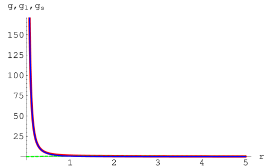
FIG. 3.: $g(r),g_{l}(r)$ and $g_{s}(r)$ plotted as thick solid line, dashed line, and thin solid line respectively. Note that $g$ and $r$ are dimensionless quantities defined in Eq. [8].

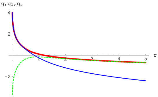
FIG. 4.: Logarithm of $g(r),g_{l}(r)$ and $g_{s}(r)$ plotted as thicker solid line, dashed line, and solid thin line respectively. Note that $g$ and $r$ are dimensionless quantities defined in Eq. [8].

In addition, one can also compute the changing rate of the gravitational field for the following equation of running gravitational field

$$\partial_{r}g=-2g^{2}{(g^{2}+1)^{3/4}\over g^{2}+2}.$$ (16)

If we define $k=1/r$ as a parameter simulating the effect of the conjugated momentum, one can also show that the changing rate $\partial_{k}g(k)$ obeys the following equation

$$\partial_{k}g=2{(g^{2}+1)^{5/4}\over g^{2}+2}$$ (17)

These equations play the role similar to the renormalization group equation for a quantum field theory. In addition, Eq. [16] also states that $g(r)$ decreases monotonically as $r$ increases. Similarly, Eq. [17] indicates that $g(k)$ increases monotonically as $k$ increases.

III Effective Potential and effective dimension

One can integrate $g$ for the effective potential. After some algebra, One can show that the effective potential $V_{l}\equiv-\int_{\infty}^{r}{\bf g}_{l}\cdot d{\bf r}=\int^{r}g_{l}dr$ and similarly for $V_{s}\equiv\int^{r}g_{s}dr$ can be evaluated directly to give

$$V_{l}=\ln{\sqrt{1+\sqrt{1+4r^{4}}}\over\sqrt{2}}-\sum_{n=1}^{\infty}{\pi_{k=1}^{n}(4k-3)\over 2n\cdot n!2^{n}(1+\sqrt{1+4r^{4}})^{n}},$$ (18)

and

$$V_{s}=-{\sqrt{1+\sqrt{1+4r^{4}}}\over\sqrt{2}r}$$ (19)

One can verify directly that $V_{l}^{\prime}=g_{l}$ and $V_{s}^{\prime}=g_{s}$ and prove that above equations are indeed correct up to an irrelevant integration constant. In fact, it is difficult to specify this constant of integration in the conventional approach which take $V(r\to\infty)\to 0$. This is because the effective potential in fact diverges at spatial infinity due to the logarithm behavior of the dominating 2D-like potential.

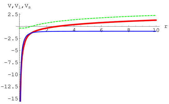
FIG. 5.: $V(r),V_{l}(r)$ and $V_{s}(r)$ plotted as thick solid line, dashed line, and thin solid line respectively.

In order to take a look at the form of these effective potential , one plots $V,V_{l},$ and $V_{s}$ together in Fig. 5. It is easy to find that $V_{l}$ has a flat plateau area when $r\to 0$ indicating that $g_{l}$ contributes little to $g$ at short distance. Similarly, one finds that the slope of $V_{s}$ becomes constant as $r\gg 1$ indicating that $g_{s}$ is significant only at short distance scale. Note that, the series sum in $V_{s}$ converges quickly. One takes $n=100$ when we plot Fig. 5.

One knows that the four dimensional space time is modified when the physical scale becomes small in the Kaluza-Klein theory. Recent evidences in MOND research seems to imply that the effective dimension of our universe decreases as the length scale increases. It is possible that Kaluza-Klein approach could play an important, but quite different, role for large scale system. The observed rotation curve of spiral galaxies indicates that the gravitational attraction goes as $1/r$ in all directions without the existence of any cosmic dark matter. This is, however, quite different from the conventional geometry of any two dimensional space. But the success of MOND seems to indicate a new direction of dimensional effect.

It is then very interesting to study how the effective dimension decreases as the observation scale increases. Therefore, one manages to define an effective dimension in this paper hoping to find our way to the discovery of the underlying theory.

Indeed, one can define the effective dimension $d(r)$ by the definition

$$g={1\over r^{d-1}}$$ (20)

such that $d\to 3$ as $r\to 0$ and $d\to 2$ as $r\to\infty$. This is a naive way to define an effective dimension such that $d$ will signify the geometric dimension as $3$-dimension and $2$-dimension respectively in a close way. It is then straightforward to show that

$$r^{d-3}={\sqrt{1+\sqrt{1+4r^{4}}}\over\sqrt{2}}$$ (21)

and hence,

$$d=2-{\sinh^{-1}{1\over 2r^{2}}\over 2\ln r}.$$ (22)

Note, however, that this definition of $d(r)$ fails to tell us anything when $r\to 1$. The reason is that $d$ is ill-defined at $r=1$ which is an obvious result of Eq. 20. One resolution to this problem is to introduce a $\Lambda$-shaped smooth function $\lambda(r)$ that peaks at $r=1$ reaching the value $\sqrt{1+\sqrt{5}}/\sqrt{2}\sim 1.27$ and reaching $1$ both at $r=0$ and $r\to\infty$ such that

$$\lambda(r)r^{d-3}={\sqrt{1+\sqrt{1+4r^{4}}}\over\sqrt{2}}$$ (23)

renders $d(r)$ well defined at $r=1$. Indeed, one can show that

$$d(r)=3-{\ln{\sqrt{1+\sqrt{1+4r^{4}}}\over\sqrt{2}}-\ln\lambda(r)\over\ln r}.$$ (24)

In short, the prescribed $\Lambda$-shaped function $\lambda(r)$ absorbs the discrepancy of the function $d(r)$ at $r=1$ in order to make the $d$ function well-defined everywhere including $r=1$. For simplicity, one will choose

$$\lambda(r)=1+[{\sqrt{1+\sqrt{5}}\over\sqrt{2}}-1]\sqrt{r}\exp[1-\sqrt{r}].$$ (25)

One can easily show that this function peaks at $r=1$ reaching the value $\sqrt{1+\sqrt{5}}/\sqrt{2}$ and reaches $1$ both at $r=0$ and $r\to\infty$ as required. And it has little effect elsewhere. This is exactly the function shown in Fig. 6. In addition, Figure 7 shows $\lambda(r)$ and $g(r)$ together for comparison.

FIG. 6.: $\Lambda$-shaped smooth function one needs is plotted as function $r$. Note that $g$ and $r$ are dimensionless quantities.

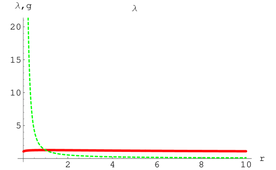
FIG. 7.: $\lambda$ and $g(r)$ are plotted as thick solid line, dashed line respectively.

Therefore, one can plot the function of effective dimension $d(r)$ in Fig. 8

FIG. 8.: effective dimension $d(r)$ is plotted as function $r$.

Note that the effective dimension function $d(r)$ does not represent the physical dimension of the theory. It only tells us roughly and effectively how the gravitational field $g$ varies as $r$ increases. In one aspect, one could view the potential as distortion of the geometry and the effective potential as the stiffness of the distorted geometry. Since the $1/r$ effect holds in all direction at large scale, not just along the disk plane, this behavior is quite different from simple geometric and dimensional deformation. All evidences indicate this sort of geometry deserves more attention.

IV conclusion

In this paper, one proposes a different view of MOND by looking at the physics related by the mass distribution and the coordinate scale of the system. In addition, one finds it useful to separate the effective gravitation field $g(r)$ into a small scale (or short-distance )$g_{s}$ field and a large scale (or a long-distance) $g_{l}$ field that should be helpful for a better understanding of the underlying physics. The effective potential is obtained accordingly.

We have also studied the changing pattern of the effective dimension $d(r)$ which will be defined as a function of the physical scale $r$. One plots this $d(r)$ functions hoping for a better understanding of the changing pattern of the effective dimension. Possible speculation with the Kaluza-Klein theory is also discussed in this paper too.

Acknowledgments This work is supported in part by the National Science Council of Taiwan.

References

References

- [1] Bekenstein, J.D. 1988, in Second Canadian Conf. on General Relativity and Relativistic Astrophysics, eds. Coley, A., Dyer, C., Tupper, T., World Scientific, Singapore, p.487
- [2] Bekenstein, J.D. & Milgrom, M. 1984, ApJ, 286, 7 (BM)
- [3] Bekenstein, J.D. & Sanders, R.H. 1994, ApJ, 286, 7
- [4] Broeils, A.H. 1992, PhD Dissertation, Univ. of Groningen
- [5] Casertano, S. & van Gorkom, J.H. 1991, AJ, 101, 1231
- [6] Deffayet, C. 2001, Phys.Lett. B 502, 199
- [7] Faber, S.M., & Jackson, R.E. 1976, ApJ, 204, 668
- [8] Falco, E.E., Kochanek, C.S., Munoz, J.A. 1998, ApJ, 494, 47
- [9] Felten, J.E. 1984, ApJ, 286, 38
- [10] Fish, R.A. 1964, ApJ, 139, 284
- [11] Freeman, K.C. 1970, ApJ, 160, 811
- [12] Hanany, S. et al. 2000, ApJ, 545, L5
- [13] Lange, A.E. et al. 2001, Phys.RevD, 63, 042001
- [14] McGaugh, S.S., de Blok, W.J.G. 1998a, ApJ, 499, 66
- [15] McGaugh, S.S., de Blok, W.J.G. 1998b, ApJ, 508, 132
- [16] McGaugh, S.S. 1999, ApJ, 523, L99
- [17] McGaugh, S.S. 2000, ApJ, 541, L33
- [18] McGaugh, S. S., Schombert, J. M., Bothun, G. D., de Blok, W. J. G. 2000, ApJ, 533, 99
- [19] Milgrom, M. 1983a, ApJ, 270, 365
- [20] Milgrom, M. 1983b, ApJ, 270, 371
- [21] Milgrom, M. 1983c, ApJ, 270, 384
- [22] Milgrom, M. 1984 ApJ, 287, 571
- [23] Milgrom, M. 1994, Ann.Phys, 229, 384
- [24] Milgrom, M. 1999, Physics Letters A, 253, 273
- [25] Ostriker, J.P. & Peebles, P.J.E. 1973, ApJ, 186, 467
- [26] Perlmutter, S. et al. 1999, ApJ, 517, 565
- [27] Sanders, R.H. 1997, ApJ, 480, 492
- [28] Sanders, R.H. 1998, MNRAS, 296, 1009
- [29] Sanders, R.H. 1999, ApJ, 512, L23
- [30] Sanders, R.H. 2000, MNRAS, 313, 767
- [31] Sanders, R.H. 2001, ApJ (in press), astro-ph/0011439
- [32] Sanders, R.H., Verheijen M.A.W. 1998 ApJ, 503, 97
- [33] Seljak, U. & Zeldarriaga, M. 1996, ApJ, 469, 437
- [34] Silk, J. 1968 ApJ, 151, 469
- [35] Solomon, P.M., Rivolo, A.R., Barrett, J., Yahil, A. 1987, ApJ, 319, 730
- [36] Tully, R.B. & Fisher, J.R. 1977, A&A, 54, 661
- [37] Tully, R.B., Verheijen, M.A.W., Pierce, M.J., Hang, J-S., Wainscot, R. 1996, AJ, 112, 2471
- [38] Verheijen, M.A.W. & Sancisi 2001, A&A, 370, 765
- [39] Weinberg, S., Gravitation and Cosmology (Wiley, New York, 1972)