A Chandra Survey of Early-type Galaxies, I: Metal Enrichment in the ISM.

Abstract

We present the first in a series of papers studying with Chandra the X-ray properties of a sample of 28 early-type galaxies which span $\sim$3 orders of magnitude in X-ray luminosity (${\rm L_{X}}$). We report emission-weighted Fe abundance (${\rm Z_{Fe}}$) constraints and, for many of the galaxies, abundance constraints for key elements such as O, Ne, Mg, Si, S and Ni. We find no evidence of the very sub-solar ${\rm Z_{Fe}}$ historically reported, confirming a trend in recent X-ray observations of bright galaxies and groups, nor do we find any correlation between ${\rm Z_{Fe}}$ and luminosity. Except in one case we do not find evidence for a multi-phase interstellar medium (ISM), indicating that multi-temperature fits required in previous ASCA analysis arose due to the strong temperature gradients which we are able to resolve with Chandra. We compare the stellar ${\rm Z_{Fe}}$, estimated from simple stellar population model fits, to that of the hot gas. Excepting one possible outlier we find no evidence that the gas is substantially more metal-poor than the stars and, in a few systems, ${\rm Z_{Fe}}$ is higher in the ISM. In general, however, the two components exhibit similar metallicities, which is inconsistent with both galactic wind models and recent hierarchical chemical enrichment simulations. Adopting standard SNIa and SNII metal yields our abundance ratio constraints imply 66$\pm$11% of the Fe within the ISM was produced in SNIa, which is remarkably similar to the Solar neighbourhood, and implies similar enrichment histories for the cold ISM in a spiral and the hot ISM in elliptical galaxies. Although these values are sensitive to the considerable systematic uncertainty in the supernova yields, they are also in very good agreement with observations of more massive systems. These results indicate a remarkable degree of homology in the enrichment process operating from cluster scales to low-to-intermediate ${\rm L_{X}}$ galaxies. In addition the data uniformly exhibit the low ${\rm Z_{O}}$/${\rm Z_{Mg}}$ abundance ratios which have been reported in the centres of clusters, groups and some galaxies. This is inconsistent with the standard calculations of metal production in SNII and may indicate an additional source of $\alpha$-element enrichment, such as Population III hypernovae.

1. Introduction

The entire history of star-formation and evolution leaves its chemical signature in the hot gas of early-type galaxies. X-ray observations therefore provide a natural and powerful diagnostic tool to unlock this information (e.g. Loewenstein & Mathews, 1991; Mathews & Brighenti, 2003). However, historically X-ray measurements of interstellar medium (ISM) abundances have been problematical, as typified by the so-called “Fe discrepancy” (Arimoto et al., 1997). Early Rosat and ASCA observations of these galaxies tended to imply extremely sub-solar metal abundances (generally expressed as ${\rm Z_{Fe}}$, the Fe abundance with respect to the adopted solar standard, since Fe has the strongest diagnostic lines in the soft X-ray band) (e.g. Loewenstein & Mushotzky, 1998), in stark contrast to $\sim$solar abundances in the stellar population. Since individual galaxies are not “closed boxes”, the ISM is believed to be built up primarily through stellar mass-loss and Type Ia supernovae (SNe) ejecta. These two crucial ingredients lead classical “wind models” of gas enrichment to predict highly super-solar ${\rm Z_{Fe}}$ in these galaxies (e.g. Ciotti et al., 1991; Loewenstein & Mathews, 1991). The problems caused by this discrepancy are exacerbated further when attempting to understand gas enrichment in clusters of galaxies, for which X-ray observations typically find ${\rm Z_{Fe}}$$\sim$0.3–0.5. The metal content of the intra-cluster medium (ICM) is primarily attributed to the stellar ejecta from giant elliptical galaxies, and so it is difficult to envisage there being lower metal abundances in individual galaxies than in the ICM (Renzini, 1997).

Attempts to reproduce the low ${\rm Z_{Fe}}$ in early-type galaxies from a modelling standpoint by, for example, incorporating ongoing accretion of unenriched gas (e.g. Brighenti & Mathews, 1999) or allowing complex star-formation histories (e.g. Kawata & Gibson, 2003) have not been entirely successful, leading some to point a finger at the spectral-modelling. Arimoto et al. (1997), for instance, called into question the plasma codes being fitted to the data, particularly in light of uncertainties associated with the Fe L-shell transitions in X-ray emission plasma codes. This point was investigated further by Matsushita et al. (2000), who argued that, having degraded the data quality in the vicinity of the Fe L-shell, ${\rm Z_{Fe}}$$\mathrel{\hbox to0.0pt{\lower 3.0pt\hbox{$\sim$}\hss}\raise 2.0pt\hbox{$>$}}$ 0.5 can be found in the highest X-ray luminosity (${\rm L_{X}}$) galaxies. Consistent results from spectral-fitting with plasma codes that treat the Fe L-shell transitions differently would seem, however, to conflict with this explanation (e.g. Buote et al., 2003b). Although remaining errors in the treatment of the Fe L-shell in the plasma codes can be important for high-resolution spectroscopy (e.g. Behar et al., 2001), at CCD resolution the effects are substantially washed out so that they contribute only a $\sim$10–20% systematic uncertainty to the abundance measurement (Buote et al., 2003b).

Perhaps a more natural alternative was suggested by Buote & Fabian (1998), who demonstrated that fitting a single temperature model to the emission spectrum of intrinsically non-isothermal hot gas gives rise to a substantially under-estimated abundance (not to mention a significantly poorer fit), an effect dubbed the “Fe bias” (see also Buote, 2000b). This effect had previously been recognized by Buote & Canizares (1994), and Trinchieri et al. (1994) found that fitting a two-temperature model to the Rosat spectrum of the bright elliptical NGC 4636 resulted in poorly-constrained abundances which could be consistent with solar values, in contrast to low ${\rm Z_{Fe}}$ required for single-temperature fits. A spectrally hard (kT$\mathrel{\hbox to0.0pt{\lower 3.0pt\hbox{$\sim$}\hss}\raise 2.0pt\hbox{$>$}}$ 5 keV) component had long been recognized in the ASCA spectra of the many early-type galaxies, which was attributed to emission from undetected X-ray binaries (Matsushita et al., 1994). The composite spectrum from these sources, which dominate the emission of low-${\rm L_{X}}$ galaxies, can typically be approximated as a pure bremsstrahlung model. Therefore, fitting only a single-temperature hot gas model to the spectra of such galaxies also tends to give rise to unphysically low abundances (e.g. Fabbiano et al., 1994; Kim et al., 1996, who found essentially unconstrained abundances when incorporating a term to account for this effect in their Rosat analysis). This effect is clearly distinct from, albeit related to, the Fe bias (see discussion in Buote, 2000b). Although the spectral-shape of the unresolved source component is sufficiently hard that it cannot move to mitigate, even in part, the Fe bias arising from multi-temperature hot gas components, Buote & Fabian (1998) still found ${\rm Z_{Fe}}$ consistent with solar in the lower-${\rm L_{X}}$ systems, in which the fit implied only a single hot gas component, plus undetected sources. However, the poor signal-to-noise ratio (S/N) characteristic of the lower-${\rm L_{X}}$ galaxies tended to produce poorly-constrained abundances, so that very sub-solar abundances could not be ruled out.

Recent Chandra and XMM measurements of abundances in X-ray bright galaxies and the centres of groups have tended to support $\sim$solar or even slightly super-solar abundances for the ISM (e.g. Buote et al., 2003b; Tamura et al., 2003; Gastaldello & Molendi, 2002; Buote, 2002; Xu et al., 2002; O’Sullivan et al., 2003; Kim & Fabbiano, 2004b). In contrast, very sub-solar ${\rm Z_{Fe}}$ are still being reported in the lowest ${\rm L_{X}}$/${\rm L_{B}}$ systems (e.g. Irwin et al., 2002; Sarazin et al., 2001). Perhaps the most dramatic examples of this latter effect are the three very low-${\rm L_{X}}$ galaxies for which O’Sullivan & Ponman (2004) reported ${\rm Z_{Fe}}$$\mathrel{\hbox to0.0pt{\lower 3.0pt\hbox{$\sim$}\hss}\raise 2.0pt\hbox{$<$}}$ 0.1. This apparent lack of consistency in the enrichment processes operating on different scales is intriguing, and it remains to be assessed whether it is an artefact of the poorer S/N or a real effect in low-${\rm L_{X}}$ systems. Although a major problem for our understanding of galaxy evolution, a full understanding of this effect is inhibited by the lack of interesting abundance constraints in galaxies with ${\rm L_{X}}$ intermediate between these two extremes. In a recent paper, Humphrey et al. (2004), we made some initial progress in this area by reporting constraints for the normal, moderate-${\rm L_{X}}$ S0 galaxy NGC 1332 and the elliptical NGC 720, in both cases strongly excluding the extremely sub-solar (${\rm Z_{Fe}}$$\mathrel{\hbox to0.0pt{\lower 3.0pt\hbox{$\sim$}\hss}\raise 2.0pt\hbox{$<$}}$ 0.4) abundances historically reported for these systems. Coupled with similar constraints on the abundances in the moderate ${\rm L_{X}}$/${\rm L_{B}}$ radio galaxy NGC 1316 (Kim & Fabbiano, 2003), this would hint at a consistent picture of enrichment from cluster to moderate-${\rm L_{X}}$ galaxy scales.

In addition to the insight into enrichment afforded from global ${\rm Z_{Fe}}$ measurements, the $\alpha$-element abundance ratios, with respect to Fe, provide an additional powerful diagnostic. Different types of SNe inject material imprinted with characteristic chemical “fingerprints”, so that the measured abundance pattern can be used to assess the relative contribution of SNIa and SNII to ISM enrichment. Early attempts to extract this information (e.g. Matsushita et al., 2000; Finoguenov & Jones, 2000) were largely affected by a failure to treat the Fe bias, although a significant contribution of SNIa to the enrichment process was indicated. More recently, studies with high-quality XMM and Chandra data have revealed typically $\sim$70–90% of the ISM enrichment in the centres of groups and clusters seems to have its origin in SNIa, which is close to the $\sim$75% value in the Solar neighbourhood (e.g. Gastaldello & Molendi, 2002; Buote et al., 2003b). For NGC 1332 and NGC 720, we were able to obtain interesting constraints on the $\alpha$-to-Fe ratios in some of the lowest-${\rm L_{X}}$ systems to date, again inferring $\sim$70–80% of the Fe to have been produced in SNIa. This also supports the suggestion of homology in the enrichment process over different mass-scales, at least down to moderate-${\rm L_{X}}$ galaxies.

Although these results are intriguing, it is by no means clear that the two galaxies we considered are representative, nor is it clear that all X-ray bright galaxies follow the trend of $\sim$solar abundances (e.g. Sambruna et al., 2004). Furthermore, these studies have not elucidated the processes which may be giving rise to very low-${\rm Z_{Fe}}$ measurements in the faintest systems. In light of these results, therefore, the next logical step is to consider a uniformly-analyzed sample of galaxies spanning a large range of ${\rm L_{X}}$, and particularly expanding the number of moderate-${\rm L_{X}}$ galaxies studied. In this paper, we present the results of a study of metal enrichment in a sample of 28 early-type galaxies drawn from the Chandra archive. In subsequent papers we will discuss the gravitating mass and point-source populations of these objects as a whole. The galaxies have been carefully selected to span the available X-ray luminosity range, from group-dominant to low-${\rm L_{X}}$ galaxies.

In many respects, Chandra ACIS is the natural instrument with which to undertake such a study. Although XMM has a significantly higher collecting area, the analysis of faint, diffuse sources is complicated by difficulties in treating the background. Chandra also has an intrinsic advantage in being able to resolve out a substantial fraction of the X-ray binary contribution into individual sources, which must otherwise be disentangled spectrally. The excellent spatial resolution of Chandra also provides an unprecedented opportunity to investigate any spatial temperature variation, which would provide the natural source of the Fe bias. Imaging spectroscopy at CCD resolution is well-suited to determine reliable abundances in a galaxy. In fact there are a number of drawbacks to using the Chandra and XMM gratings instead for such a study. The extended nature of the sources makes grating spectroscopy extremely challenging. The significantly lower effective area of the grating spectrographs in comparison to the ACIS CCDs and, especially for the XMM RGS instrument, the more limited bandwidth both exacerbate this problem. Although one of the key issues of interest is the determination of multiple temperature components in the extraction aperture, this tends to produce features broad enough to be evident in CCD spectra. In fact, based on high S/N data of the group NGC 5044 there was excellent agreement in the abundances determined with the XMM gratings and the XMM and Chandra CCDS (Buote et al., 2003b; Tamura et al., 2003), confirming that CCD resolution is sufficient to obtain reliable abundances.

Throughout this paper we adopt the latest solar abundances standard of Asplund et al. (2004, see § 4.1), which resolve several previously-noted discrepancies between “photospheric” and “meteoritic” values. All error-bars quoted refer to the 90% confidence region, unless otherwise stated.

2. Target Selection

By its nature, the Chandra archive contains a nonuniform sample of galaxies. Although this prevents our choosing a statistically complete sample, we selected 28 galaxies approximately spanning the range of measured ${\rm L_{X}}$, from $\sim 8\times 10^{39}$–$10^{43}$${\rm erg\ s^{-1}}$. We only considered relatively nearby galaxies which had been observed for a total of at least 10 ks with the ACIS-S or ACIS-I, and without any grating employed. For selection purposes X-ray luminosities were taken from the catalogue of O’Sullivan et al. (2001), although all luminosities have subsequently been recomputed in the present work (§ 3.2). To an initial sample of 26 galaxies chosen in this way, we also added two further interesting objects not in the O’Sullivan catalogue— NGC 1132, one of the closest examples of a “fossil group” (Mulchaey & Zabludoff, 1999, F. Gastaldello et al, 2005, in prep.) and the relatively isolated, moderate-${\rm L_{X}}$ galaxy NGC 1700 which has an unusually high X-ray ellipticity, which Statler & McNamara (2002) argued may indicate rotational support. Two of our sample, NGC 1332 and NGC 720, have already been discussed in Humphrey et al. (2004), and we adopt the results from that work here. The sample contains 10 high-${\rm L_{X}}$ (${\rm log_{10}}$${\rm L_{X}}$$\mathrel{\hbox to0.0pt{\lower 3.0pt\hbox{$\sim$}\hss}\raise 2.0pt\hbox{$>$}}$ 41.5) galaxies, 12 moderate-${\rm L_{X}}$(${\rm log_{10}}$${\rm L_{X}}$$\simeq$40.5–41.5) and 6 low-${\rm L_{X}}$ (${\rm log_{10}}$${\rm L_{X}}$$\mathrel{\hbox to0.0pt{\lower 3.0pt\hbox{$\sim$}\hss}\raise 2.0pt\hbox{$<$}}$ 40.5 ) galaxies. Most of the sample was observed with ACIS-S, although in a few cases ACIS-I was employed. To give extra coverage at large radii both ACIS-S and ACIS-I data for the two bright galaxies NGC 1399 and NGC 4472, were analysed together.

A summary of the properties of the galaxies and details of the Chandra exposures are given in Table 1. In order to provide accurate luminosity estimates, we searched the literature for reliable distance estimates. Where possible, we adopted those determined from surface brightness fluctuations (SBF) by Tonry et al. (2001, correcting for an improved Cepheid zero-point: ) or Jensen et al. (2003). Alternatively, we used distances determined from the ${\rm D_{n}-\sigma}$ relation (Faber et al., 1989), or the redshift, corrected for Virgo-centric flow, as given in LEDA. We assumed ${\rm H_{0}}$=70 ${\rm km\ s^{-1}\ Mpc^{-1}}$.

Of this sample, 6 systems (IC 4296, NGC 507, NGC 741, NGC 1399, NGC 4472, NGC 7619) appear to be the central galaxies in substantial, optically-identified groups so their X-ray emission may be to some extent intertwined with that of a surrounding intra-group medium (IGM). In the present context, it suffices to consider that all the systems comprise a continuum over a range of mass-scales. In a subsequent paper, we will discuss the issue of group membership, and the total gravitating mass, in detail.

Table 1The sample

Galaxy	Type	Dist	${\rm D_{25}}$	${\rm L_{B}}$	log10${\rm L_{X}}$	$N_{\rm H}$	ObsID	Instr.	Date	Exposure
		(Mpc)	(′)	($10^{10}$${\rm L_{\odot}}$)	(${\rm log_{10}(erg\ s^{-1})}$)	(${\rm 10^{20}cm^{-2}}$)			(dd/mm/yy)	(ks)
High-${\rm L_{X}}$ galaxies
IC 4296	E Radio gal	50.82	3.8	12.1	41.54	4.1	3394	S	10/09/01	25
NGC 507	SA(r)0	82.63	3.2	14.9	43.03	5.4	2882	I	08/01/02	43
NGC 741	E0	75.83	2.9	14.2	42.32	4.4	2223	S	28/01/01	30
NGC 1132	E	98.24	2.1	8.3	42.76	5.2	801	S	10/12/99	13
NGC 1399	cD;E1 pec	18.51	6.9	4.2	42.09	1.3	319	S	18/01/00	56
							4174	I	28/05/03	45
NGC 1600	E3	57.43	3.2	9.8	42.19	4.8	4283	S	18/09/02	22
NGC 4472	E2/S0(2) Sy2	15.11	9.7	7.5	41.52	1.7	321	S	12/06/00	32
							322	I	19/03/00	10
NGC 5846	E0-1;LINER HII	21.11	3.8	3.1	41.57	4.3	788	S	24/05/00	23
NGC 7619	E	49.21	2.6	6.9	42.06	5.0	3955	S	24/09/03	31
NGC 7626	E pec	51.23	2.7	6.9	41.51	5.0	2074	I	20/08/01	26
Moderate-${\rm L_{X}}$ galaxies
NGC 720	E5	25.71	4.6	3.1	41.33	1.5	492	S	12/10/00	29
NGC 1332	S(s)0	21.31	4.1	2.3	40.95	2.2	4372	S	19/09/02	45
NGC 1387	SAB(s)0	18.91	3.3	1.2	40.78	1.3	4168	I	20/05/03	45
NGC 1407	E0	26.81	5.3	6.5	41.32	5.4	791	S	16/08/00	40
NGC 1549	E0-1	18.31	4.7	2.9	40.66	1.5	2077	S	08/11/00	22
NGC 1553	SA(rl)0 LINER	17.21	5.3	3.7	40.64	1.5	783	S	02/01/00	14
NGC 1700	E4	41.1${}^{1}\dagger$	3.0	4.6	41.20	4.8	2069	S	03/11/00	27
NGC 3607	SA(s)0	21.21	4.5	3.4	40.94	1.5	2073	I	12/06/01	38
NGC 3923	E4-5	21.31	6.4	4.9	41.03	1.5	1563	S	14/06/01	8.8
NGC 4365	E3	19.01	5.8	3.7	40.83	6.2	2015	S	02/06/01	40
NGC 4552	E;LINER HII	14.31	5.0	2.0	40.65	2.6	2072	S	22/04/01	54
NGC 5018	E3	42.63	3.6	7.1	40.96	7.0	2070	S	14/04/01	28
Low-${\rm L_{X}}$ galaxies
NGC 3115	S0	9.01	7.3	1.4	39.86	4.3	2040	S	14/06/01	36
NGC 3585	E7/S0	18.61	6.1	3.3	40.35	5.6	2078	S	03/06/01	35
NGC 3608	E2 LINER	21.31	3.2	1.7	40.39	1.5	2073	I	12/06/01	38
NGC 4494	E1-2 LINER	15.81	4.5	2.3	40.36	1.5	2079	S	05/08/01	15
NGC 4621	E5	17.01	5.0	2.5	40.14	2.2	2068	S	01/08/01	25
NGC 5845	E	24.01	0.9	0.45	40.17	4.3	4009	S	03/01/03	30

Note. — Listed above are all of the galaxies in our sample. Distances were obtained from ¹— SBF: Tonry et al. (2001), corrected for the the new Cepheid zero-point (see text), ²— SBF: Jensen et al. (2003), ³— ${\rm D_{n}}$-$\sigma$: Faber et al. (1989), ⁴— redshift distance (LEDA); $\dagger$— uncertain. ${\rm L_{B}}$ was determined from the face-on, reddening-corrected B-band magnitude given by LEDA. ${\rm L_{X}}$ was computed in the 0.1–10.0 keV band self-consistently in the present work(§ 3.2), excluding obvious emission from any low-luminosity AGN, and extrapolating the surface brightness to a fiducial 300 kpc radius. The galaxy type was taken from NED. $N_{\rm H}$ is the nominal Galactic column-density along the line-of-sight. We show the Chandra observation identifier (ObsID), the ACIS instrument (I or S) and the net exposure-time, having excluded periods of flaring.

3. Data reduction

For data reduction we used the CIAO 3.1 and Heasoft 5.3 software suites, in conjunction with Chandra Caldb calibration database 2.28. For spectral-fitting we used Xspec 11.3.1. In order to ensure the most up-to-date calibration, all data were reprocessed from the “level 1” events files, following the standard Chandra data-reduction threads. We applied corrections to take account of a time-dependent drift in the satellite gain and, for ACIS-I observations, the effects of “charge transfer inefficiency”, as implemented in the standard CIAO tools.

To identify periods of enhanced background (“flaring”), which seriously degrades the signal-to-noise (S/N) and complicates background subtraction (e.g. Markevitch, 2002), we accumulated background lightcurves for each exposure from low surface-brightness regions of the active chips. We excluded obvious diffuse emission and data in the vicinity of any detected point-sources (see below). Periods of flaring were identified by eye and excised. Any residual flaring which is not removed by this procedure will be sufficiently mild to have negligible impact in the centres of bright galaxies. However, in the fainter systems even very mild background variation can have a significant impact on our results, and so we treat these systems with extra care (§ 5.2). The final exposure times are listed in Table 1.

Point source detection was performed using the CIAO tool wavdetect (Freeman et al., 2002). In order to improve the likelihood of identifying sources with peculiarly hard or soft spectra, full-resolution images were created of the region of the ACIS focal-plane containing the S3 chip in the energy-band 0.1–10.0 keV and, so as to identify any unusually soft or hard sources, also in the bands 0.1–3.0 keV and 3.0–10.0 keV. Sources were detected separately in each image. In order to minimize spurious detections at node or chip boundaries we supplied the detection algorithm with exposure-maps generated at energies 1.7 keV, 1.0 keV and 7 keV respectively (although the precise energies chosen made little difference to the results). The detection algorithm searched for structure over pixel-scales of 1, 2, 4, 8 and 16 pixels, and the detection threshold was set to $\sim 10^{-7}$ spurious sources per pixel (corresponding to $\sim$0.1 spurious detections per image). The source-lists obtained within each energy-band were combined and duplicated sources removed, and the final list was checked by visual inspection of the images. A full discussion of the point source populations will be given in a subsequent paper. In the present work, the data in the vicinity of any detected point source were removed so as not to contaminate the diffuse emission. As discussed in Humphrey & Buote (2004, see also ) a significant fraction of faint X-ray binary sources will not have been detected by this procedure, and so we include an additional component to account for it in our spectral fitting.

3.1. Background estimation

One of the key challenges in spectral-fitting diffuse X-ray emission is ensuring proper background subtraction. For Chandra a set of blank-field event files have been made available as part of the standard Caldb distribution, from which background spectra can be accumulated corresponding to similar regions of the detector. For each observation, we prepared from these a suitably projected background events file. We were able to extract from this file “template” background spectra for each region of the detector in which our “source” spectra were obtained. However, these background spectra are unlikely to represent perfectly the background in any one observation. There are known to be significant long-term secular variations in the non X-ray components of the background, substantial field-to-field variation in the cosmic component, and there may be some residual mild flaring. It is also worth noting that the hard (power law) component of the cosmic X-ray background arises from undetected background AGN, so its absolute normalization is also a strong function of the point source detection completeness; in turn this is a function of the surface brightness of the galaxy and the total exposure time (Kim & Fabbiano, 2004a).

Several authors have adopted the practice of renormalizing the background template to ensure good agreement with the instrumental background at high energies ($\mathrel{\hbox to0.0pt{\lower 3.0pt\hbox{$\sim$}\hss}\raise 2.0pt\hbox{$>$}}$ 10 keV). Such a procedure, however, also renormalizes the (uncorrelated) cosmic X-ray background and instrumental line features, which can lead to serious over or under-subtraction. Given these reservations we chose to use an alternative background estimation procedure. Our method involved modelling the background, somewhat akin to the approach of Buote et al. (2004). For each observation, we extracted a spectrum from a “source free” region of the ACIS field of view. We chose a $\sim$2^′ region centred on the S1 chip if the galaxy was centred on S3, or on the S2 chip where the galaxy was centred on ACIS-I. If the S1 or S2 chips were turned off, we chose a small, $\mathrel{\hbox to0.0pt{\lower 3.0pt\hbox{$\sim$}\hss}\raise 2.0pt\hbox{$<$}}$ 1^′ region on the S3 or ACIS-I chips, as appropriate, positioned to be in a region of as low surface-brightness as possible. We excluded data from the vicinity of any point-sources found by the source detection algorithm. Additionally, we extracted a “source+background” spectrum from the CCD on which the source was centred, in an annulus centred at the galaxy centroid and with an inner and outer radii typically $\sim$2.5^′ and 3.3^′. We adopted two spectra since we found that this procedure enabled us most cleanly to constrain the background. Some of the brightest galaxies are so extended in the X-ray that even in our “source free” region there is a small contribution from hot gas at large radii. We found that using two spectra with different hot gas contributions allowed this to be readily disentangled from the actual background components. In order to constrain the model, we fitted both spectra simultaneously, without background subtraction, using Xspec. Our model consisted of a single APEC plasma (to take account of the diffuse emission from the galaxy; the “source”), plus background components. These comprised a power law with $\Gamma=1.41$ (to account for the hard X-ray background), two APEC models with solar abundances and kT$=$ 0.2 and 0.07 keV (to account for the soft X-ray background) and, to model the instrumental contribution, a broken power law model and two Gaussian lines with energies 1.7 and 2.1 keV and negligible intrinsic widths. We have found that this model can be used to parameterize adequately the template background spectra.

In order to disentangle the source and background components, given the general lack of photons in these spectra, we tied the abundances and temperatures of the “source” APEC components between both extraction regions, but allowed the normalizations to be free. In the fainter galaxies the normalization of the source component in the “source free” region tended, as expected, to zero. We also assumed that the background model normalization scales exactly with the extraction area. In general, we found that this was able to fit both spectra very well. In our subsequent spectral analysis, we did not background-subtract the data using the standard templates, but took into account the background by using an appropriately scaled version of this model.

Even if the background spectrum varies substantially over the field-of-view, our background modelling is most correct at largest distances from the source centroid, where the results are most sensitive to the background. In fact, we found that the standard background templates fared much worse than these modelled background estimates when the data were from regions of low surface brightness. We discuss this issue further, and how the choice of background can affect our results in § 5.2.

3.2. ${\rm L_{X}}$ estimation

In order to provide a self-consistent analysis of the galaxies in this sample, we obtained estimates of ${\rm L_{X}}$ based on the Chandra data. First, we estimated the flux within our chosen spectral extraction regions from our the best-fitting spectral models (§ 4.3–4.4). Fluxes were computed separately for the gas and undetected point-sources in the energy-band 0.1–10.0 keV. Since the adopted aperture will not contain all of the diffuse flux from the galaxy, we extrapolated the emission out to a projected radius of 300 kpc, i.e. the Virial radius for a $1.6\times 10^{12}$${\rm M_{\odot}}$galaxy. We assumed spherical symmetry and parameterized the surface brightness with a single or double $\beta$-model. The $\beta$-model parameters were determined from fits to the radial surface brightness in the 0.3–2.0 keV band, using dedicated software which can fold in the instrumental point-spread function, which we computed at 1 keV. Data from the vicinity of any detected point-sources were excluded from the fit, and we assumed that the hot gas and undetected sources had the same radial brightness distribution. The results of the surface brightness fits to each galaxy will be discussed in detail in a subsequent paper. This procedure typically corrects the flux upwards by a factor $\sim$1.1–4, depending on the shape of the surface brightness profile. Since it is by no means certain that this extrapolation is valid out to $\sim$300 kpc, we expect this to introduce some uncertainty into the estimated ${\rm L_{X}}$. However, for our present purposes we believe this approach is sufficiently accurate.

To compute the total ${\rm L_{X}}$ of the galaxy, we also included the flux of all detected point-sources within the B-band twenty-fifth magnitude (${\rm D_{25}}$) isophote, all of which were assumed to be associated with the galaxy for these purposes. We fitted the composite spectrum of all these sources with our canonical (kT=7.3 keV bremsstrahlung) model. In most cases this gave a good fit to the data, although in a few instances a single power law or power law plus disk blackbody components were used instead to obtain a good fit. In the event a significant low-luminosity AGN appears to be present in the galaxy (i.e. NGC 1553, IC 4296), we omitted the flux from the AGN. The total luminosity of the (detected, plus undetected) point-sources within ${\rm D_{25}}$ was typically in agreement with the estimate of Kim & Fabbiano (2004a), based on extrapolating the resolved X-ray luminosity functions in nearby early-type galaxies. We found a mean ${\rm L_{X}}$(point sources)/${\rm L_{B}}$$\sim 0.9\times 10^{30}$${\rm erg\ s^{-1}}$${\rm L_{\odot}}$^-1, in excellent agreement with these authors. The point-source populations will be discussed in detail in a subsequent paper.

Comparing with the fluxes given in O’Sullivan et al. (2001) we find broad agreement, although our estimates tend to be $\sim$0.25 dex higher. We attribute this discrepancy to differences in spectral modelling and our extrapolation procedure.

4. Spectral analysis

Table 2Emission-weighted average abundances

Galaxy	$\chi^{2}$/dof	${\rm Z_{Fe}}$	${\rm Z_{O}}$/${\rm Z_{Fe}}$	${\rm Z_{Ne}}$/${\rm Z_{Fe}}$	${\rm Z_{Mg}}$/${\rm Z_{Fe}}$	${\rm Z_{Si}}$/${\rm Z_{Fe}}$	${\rm Z_{S}}$/${\rm Z_{Fe}}$	${\rm Z_{Ni}}$/${\rm Z_{Fe}}$
High-${\rm L_{X}}$ galaxies
IC 4296	54.3/68	1.8($>0.94$)	0.0($<0.53$)	…	1.04$\pm 0.47$	1.3$\pm 0.6$	…	4.8($>0.2$)
		[${}^{+0.2}_{-0.1}$]	[+0.05]	…	[$\pm 0.2$]	[${}^{+0.03}_{-0.1}$]	…	[$\pm 1.7$]
NGC 507	857/789	0.53$\pm 0.07$†	0.0($<0.26$)	0.52${}^{+0.98}_{-0.52}$	0.81 $\pm$0.22	$0.96\pm 0.13$	1.51$\pm$0.30	2.77${}^{+0.83}_{-0.70}$
		[${}^{+0.14}_{-0.08}$]	[+0.6]	[${}^{+0.26}_{-0.56}$]	[${}^{+0.13}_{-0.50}$]	[${}^{+0.1}_{-0.2}$]	[${}^{+0.2}_{-0.4}$]	[${}^{+0.7}_{-1.5}$]
NGC 741	$189.9/192$	1.19${}^{+0.95}_{-0.62}$†	$0.37^{+0.25}_{-0.30}$	…	$0.81^{+0.29}_{-0.48}$	$0.98\pm 0.35$	…	$4.0^{+1.0}_{-2.0}$
		[$\pm 0.5$]	[$\pm 0.20$]	…	[$\pm 0.15$]	[${}^{+0.12}_{-0.05}$]	…	[${}^{+1.3}_{-0.8}$]
NGC 1132	239.8/210	0.82${}^{+0.29}_{-0.20}$	0.44$\pm 0.37$	…	0.70$\pm 0.42$	1.26${}^{+0.39}_{-0.34}$	…	3.6$\pm 1.4$
		[${}^{+0.12}_{-0.15}$]	[${}^{+0.27}_{-0.18}$]	…	[${}^{+0.17}_{-0.29}$]	[${}^{+0.08}_{-0.3}$]	…	[${}^{+1.2}_{-2.2}$]
NGC 1399	1734/1223	$1.19\pm 0.10$†	$0.41\pm 0.06$	$0.64\pm 0.25$	$0.76\pm 0.08$	$0.84\pm 0.06$	1.14$\pm$0.12	2.61$\pm 0.32$
		[${}^{+0.6}_{-0.4}$]	[${}^{+0.13}_{-0.11}$]	[${}^{+0.05}_{-0.58}$]	[${}^{+0.08}_{-0.22}$]	[${}^{+0.05}_{-0.17}$]	[${}^{+0.10}_{-0.49}$]	[${}^{+0.4}_{-1.0}$]
NGC 1600	151/158	2.1$\pm 1.3$†	0.10($<0.81$)	…	0.92${}^{+0.77}_{-0.53}$	0.85${}^{+0.68}_{-0.36}$	…	1.9($>0.3$)
		[${}^{+1.3}_{-0.8}$]	[${}^{+0.38}_{-0.10}$]	…	[${}^{+0.28}_{-0.13}$]	[${}^{+0.38}_{-0.05}$]	…	[${}^{+1.2}_{-0.9}$]
NGC 4472	785/740	$1.4^{+1.7}_{-0.4}$†	0.51$\pm$0.12	0.95 $\pm 0.44$	1.02$\pm$0.11	1.25$\pm$0.11	2.36$\pm$0.33	3.28$\pm 0.61$
		[${}^{+1.7}_{-0.6}$]	[${}^{+0.07}_{-0.03}$]	[${}^{+0.17}_{-0.28}$]	[${}^{+0.07}_{-0.1}$]	[${}^{+0.1}_{-0.2}$]	[${}^{+0.3}_{-0.7}$]	[${}^{+0.7}_{-1.8}$]
NGC 5846	558/432	$3.0^{+1.8}_{-0.5}$	0.20$\pm 0.13$	0.88${}^{+0.61}_{-0.58}$	0.75$\pm 0.12$	0.78${}^{+0.14}_{-0.11}$	1.14${}^{+0.46}_{-0.38}$	1.92${}^{+1.81}_{-1.14}$
		[${}^{+0.3}_{-1.0}$]	[${}^{+0.03}_{-0.04}$]	[${}^{+0.17}_{-0.32}$]	[${}^{+0.11}_{-0.05}$]	[${}^{+0.17}_{-0.010}$]	[${}^{+0.4}_{-0.2}$]	[${}^{+2.5}_{-1.1}$]
NGC 7619	279/299	2.0${}^{+2.5}_{-0.9}$	0.23${}^{+0.37}_{-0.22}$	…	1.06$\pm 0.22$	0.91$\pm 0.25$	…	0.90${}^{+1.43}_{-0.90}$
		[${}^{+3.0}_{-0.3}$]	[${}^{+0.23}_{-0.04}$]	…	[${}^{+0.3}_{-0.1}$]	[${}^{+0.10}_{-0.08}$]	…	[${}^{+1.10}_{-0.33}$]
NGC 7626	59.6/45	0.37${}^{+0.60}_{-0.16}$	…	…	1.2${}^{+0.88}_{-0.94}$	1.3$\pm 1.0$	…	…
		[${}^{+1.30}_{-0.19}$]	…	…	[${}^{+0.5}_{-0.4}$]	[${}^{+0.9}_{-0.2}$]	…	…
Moderate-${\rm L_{X}}$ galaxies
NGC 7201	383.4/357	$0.80^{+0.45}_{-0.24}$	0.30$\pm 0.28$	0.68$\pm 0.67$	1.26$\pm 0.35$	…	…	…
		[${}^{+2.00}_{-0.35}$]	[${}^{+0.03}_{-0.30}$]	[${}^{+0.06}_{-0.68}$]	[${}^{+0.35}_{-0.16}$]	…	…	…
NGC 13321	189.4/174	$1.2^{+1.9}_{-0.4}$	0.08${}^{+0.13}_{-0.08}$	1.53$\pm 0.31$	1.07$\pm 0.27$	0.87$\pm 0.49$	…	…
		[$\pm 0.3$]	[$\pm 0.4$]	[$\pm 0.1$]	[$\pm 0.3$]	[$\pm 0.2$]	…	…
NGC 1387	61.4/61	0.38${}^{+0.56}_{-0.15}$	0.32($<1.5$)	…	0.18${}^{+0.46}_{-0.18}$	0($<$0.51)	…	…
		[${}^{+1.4}_{-0.14}$]	[${}^{+0.89}_{-0.32}$]	…	[${}^{+0.23}_{-0.04}$]	[+0.1]	…	…
NGC 1407	222/221	2.1${}^{+1.1}_{-0.9}$†	0.37${}^{+0.21}_{-0.25}$	…	1.10$\pm 0.23$	1.21${}^{+0.31}_{-0.27}$	2.2$\pm 1.1$	3.3${}^{+1.7}_{-1.3}$
		[${}^{+3.2}_{-0.3}$]	[$\pm 0.11$]	…	[${}^{+0.2}_{-0.09}$]	[${}^{+0.2}_{-0.1}$]	[${}^{+0.5}_{-1.2}$]	[${}^{+0.7}_{-1.7}$]
NGC 1549	9.6/18	0.17($>0.06$)	…	…	…	…	…	…
		[${}^{+4.0}_{-0.07}$]	…	…	…	…	…	…
NGC 1553	35.8/35	$0.14^{+0.09}_{-0.04}$	0.65${}^{+0.47}_{-0.31}$	1.70${}^{+0.55}_{-0.47}$	…	…	…	…
		[${}^{+0.14}_{-0.02}$]	[${}^{+0.21}_{-0.16}$]	[${}^{+0.1}_{-0.4}$]	…	…	…	…
NGC 1700	33/36	5($>0.67$)	0.31${}^{+0.49}_{-0.31}$	0.70$\pm 0.37$	0.64$\pm 0.50$	…	…	…
		[-4.0]	[$\pm 0.16$]	[${}^{+0.09}_{-0.45}$]	[${}^{+0.25}_{-0.15}$]	…	…	…
NGC 3607	43.0/41	0.32${}^{+0.60}_{-0.14}$	…	…	0.63$\pm$0.63	…	…	…
		[${}^{+1.2}_{-0.11}$]	…	…	[${}^{+0.29}_{-0.33}$]	…	…	…
NGC 3923	31.0/35	1.15($>0.27$)	0.12${}^{+0.39}_{-0.12}$	1.48${}^{+0.49}_{-0.39}$	0.85$\pm 0.45$	4.1($>2.1$)	…	…
		[${}^{+3.4}_{-0.09}$]	[${}^{+0.04}_{-0.01}$]	[${}^{+0.1}_{-1.2}$]	[${}^{+0.08}_{-0.19}$]	[${}^{+0.2}_{-1.9}$]	…	…
NGC 4365	43.3/45	5.0($>0.76$)	0.46${}^{+1.76}_{-0.36}$	…	0.87$\pm 0.88$	…	…	…
		[$-3.4$]	[${}^{+1.64}_{-0.02}$]	…	[${}^{+0.58}_{-0.77}$]	…	…	…
NGC 4552	139/143	$0.71^{+0.27}_{-0.10}$	0.17${}^{+0.11}_{-0.06}$	$0.62\pm 0.22$	0.76$\pm 0.11$	1.1$\pm 0.4$	…	2.7$\pm$2.2
		[${}^{+0.26}_{-0.15}$]	[${}^{+0.21}_{-0.03}$]	[$\pm 0.15$]	[${}^{+0.31}_{-0.04}$]	[${}^{+0.3}_{-0.1}$]	…	[$\pm 1.4$]
NGC 5018	23.0/24	0.30($>0.14$)	…	…	…	…	…	…
		[${}^{+0.41}_{-0.11}$]	…	…	…	…	…	…
Low-${\rm L_{X}}$ galaxies
NGC 3115	38.2/36	0.26($>0.08$)	…	…	…	…	…	…
		[${}^{+3.0}_{-0.15}$]	…	…	…	…	…	…
NGC 3585	33.6/27	0.63($>0.12$)	…	…	…	…	…	…
		[${}^{+4.3}_{-0.49}$]	…	…	…	…	…	…
NGC 3608	33.8/23	1.1($>0.14$)	…	…	…	…	…	…
		[$\pm 1.0$]	…	…	…	…	…	…
NGC 4494	11.0/14	0.28($>0.02$)	…	…	…	…	…	…
		[${}^{+4.7}_{-0.21}$]	…	…	…	…	…	…
NGC 4621	6/9	0.31($>0$)	…	…	…	…	…	…
		[${}^{+4.7}_{-0.2}$]	…	…	…	…	…	…
NGC 5845	15.2/14	0.62($>0.13$)	…	…	…	…	…	…
		[${}^{+4.4}_{-0.5}$]	…	…	…	…	…	…

Note. — The best-fitting globally-averaged (see §4.3) emission-weighted abundances and abundance ratios for each galaxy, shown along with the quality of fit. Statistical errors represent the 90% confidence region. Figures given in square brackets are an estimate of the sensitivity of each measurement to possible sources of systematic error (see § 5). Since we did not assess them for all galaxies in the sample, calibration uncertainties (§ 5.1) are not included in this error-budget for most of the sample. These should certainly not be added in quadrature with the statistical errors. Where we were able to obtain an abundance gradient (§ 4.3), we estimated an emission-weighted ${\rm Z_{Fe}}$, extrapolated over a large aperture (see text); those affected galaxies are marked (^†). ¹—results taken from Humphrey et al. (2004), corrected to our adopted abundance standard. Where parameters could not be constrained, they were fixed at the Solar value, and listed as (…).

4.1. Solar abundances standard

Throughout this paper, we adopt the solar photospheric abundances of Asplund et al. (2004), which deviate significantly for many of the key species from the previous standard of Grevesse & Sauval (1998). The incorporation of detailed 3D line transfer modelling (and, in some cases, treatment of non-LTE conditions) has tended to reconcile so-called “meteoritic” and photospheric abundances (for non-volatile species), so that discrepancies remaining are typically at $\mathrel{\hbox to0.0pt{\lower 3.0pt\hbox{$\sim$}\hss}\raise 2.0pt\hbox{$<$}}$ 0.1 dex, i.e. approximately the same level as the statistical uncertainties. We therefore adopt these abundances as our standard. This does, however, introduce some complications when comparing with results reported in the literature since most authors adopt either the older abundances standard of Grevesse & Sauval (1998) or the outdated abundances of Anders & Grevesse (1989).

For comparison with our work, ${\rm Z_{Fe}}$, ${\rm Z_{O}}$/${\rm Z_{Fe}}$, ${\rm Z_{Ne}}$/${\rm Z_{Fe}}$, ${\rm Z_{Mg}}$/${\rm Z_{Fe}}$, ${\rm Z_{Si}}$/${\rm Z_{Fe}}$, ${\rm Z_{S}}$/${\rm Z_{Fe}}$ and ${\rm Z_{Ni}}$/${\rm Z_{Fe}}$ referenced to the standard of Grevesse & Sauval (1998) should be scaled by 1.12, 1.32, 1.55, 1.00, 0.98, 1.38 and 0.93, respectively. Likewise, these abundances obtained with the outdated standard of Anders & Grevesse (1989) should be scaled by 1.66, 1.12, 1.07, 0.68, 0.66, 0.71 and 0.63, respectively.

4.2. Error-bar estimation

It is worth noting that the error-bars generated simply with Xspec tend to underestimate substantially the true confidence region. This seems to arise because the fitting algorithms employed often spuriously identify fit convergence (regardless of how low one sets the “critical delta-fit statistic” parameter). This problem can be mitigated by re-starting the fit a number of times from the apparent minimum and ensuring that the fit statistic has truly minimized. Unfortunately the error-bar estimation routines assume that a single iteration of the fitting algorithm is sufficient to characterize the shape of the $\chi^{2}$-space, which is seldom true. Since the failure to converge results in an inflated $\chi^{2}$ for any given value of an interesting parameter, this produces error-bars which are systematically too small, sometimes dramatically so.

We experimented with two strategies to overcome this problem, which we found to agree well in general. In our preferred technique, we used a script to emulate the behaviour of the Xspec “error” command, but minimizing $\chi^{2}$ at each step with multiple iterations of the fit command (until the $\chi^{2}$ converged within a tolerance of 0.001). This has the advantage of identifying (small) local minima. The alternative method, extensively employed in our previous papers (e.g. Buote et al., 2003b) involves performing Monte-Carlo simulations in which spectra are simulated from the best-fit model. The best-fit model is then fitted to each simulated dataset and the confidence region inferred from the distribution of the best-fitting parameter values. Provided the fit statistic is well-described by the $\chi^{2}$ distribution, both techniques are statistically equivalent.

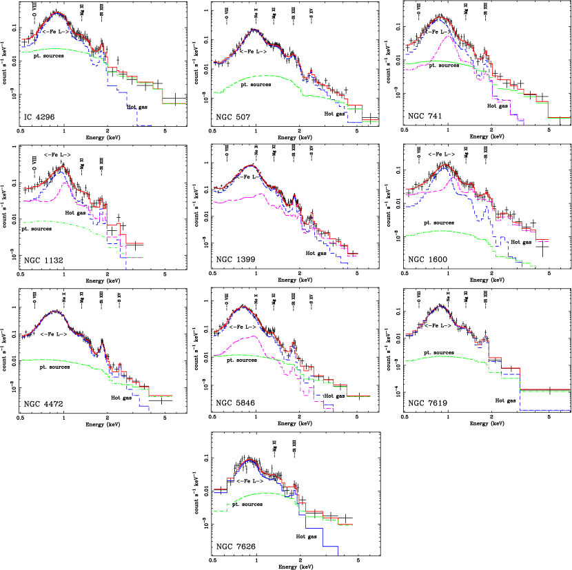
Figure 1.— Spectra of the high-${\rm L_{X}}$ galaxies. Where spatially-resolved spectroscopy was possible, only the central bin is shown, for clarity. In addition we show the best-fit model folded through the instrumental response (solid line; red), and the contribution from undetected point sources (dash dot line; green) and the one or two hot-gas components (dashed lines; blue and magenta). The energies of interesting line features are included to guide the eye.

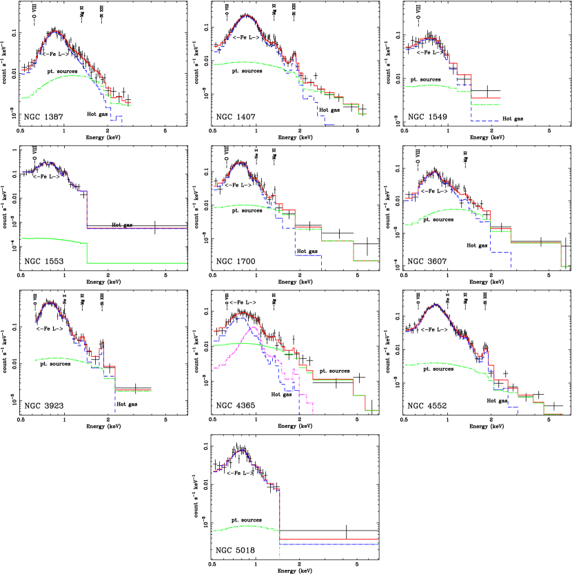
Figure 2.— Spectra of the moderate-${\rm L_{X}}$ galaxies. Note that the point-source component for NGC 1553 and NGC 5018 appears to be very small; however the error-bars on the normalization of this component are considerable.

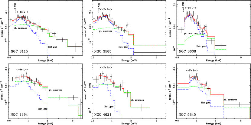
Figure 3.— Spectra of the low-${\rm L_{X}}$ galaxies.

4.3. Spatially-resolved spectroscopy

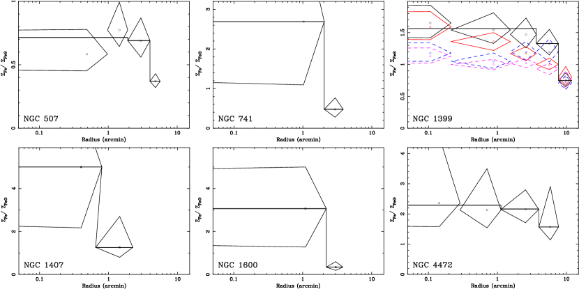
Figure 4.— The Fe abundance profiles, for those systems in which an abundance gradient was measured. Also shown are the best-fitting models used to infer a global emission-weighted abundance (§ 4.3). To demonstrate the Fe bias and the importance of deprojection, we show separately for NGC 1399 the profile obtained when two hot gas components were used in those annuli requiring them (solid lines) and when only a single hot gas component is used (dotted lines). We also show results for which deprojection was used (marked with squares) and for which deprojection was not (marked with triangles).

Where the data were of sufficient quality, we extracted spectra in a number of concentric annuli, centred on the nominal X-ray centroid. We determined the centroid iteratively by placing a 0.5^′ radius aperture at the nominal galaxy position (obtained from NED) and computing the X-ray centroid within it. The aperture was moved to the newly-computed centroid, and the procedure repeated until the computed position converged. Typically the X-ray centroid agreed with that from NED. The widths of the annuli were chosen so as to contain approximately the same number of background-subtracted photons and ensure there were sufficient photons in each to perform useful spectral-fitting. We restricted the fits to the energy-band 0.5–7.0 keV, to minimize instrumental background, which dominates at high energies, and to avoid calibration uncertainties at lower energies (however, see § 5.4). The spectra were rebinned to ensure a signal-to-noise ratio of at least 3 and at minimum 20 photons per bin (to validate $\chi^{2}$-fitting).

We fitted the spectra using Xspec with a model comprising a hot gas (vapec) component, plus an additional 7.3 keV bremsstrahlung component to take account of undetected point-source emission (this model gives a good fit to the detected sources in nearby galaxies: Irwin et al. 2003). We used a slightly modified form of the existing Xspec vapec implementation so that ${\rm Z_{Fe}}$ is determined directly, but for the remaining elements the fit parameters were the abundance ratios (in solar units) with respect to Fe. This model enabled errors on the abundance ratios to be determined directly from Xspec. In general, the data did not enable us to constrain any abundance ratio gradients, and so we tied the abundance ratios between all annuli. The absorbing column density ($N_{\rm H}$) was fixed at the Galactic value (Dickey & Lockman, 1990); the effect of varying $N_{\rm H}$ is discussed in § 5.6. Where abundances could not be constrained, they were fixed at the Solar value. We took account of possible hot gas spectral projection effects by employing the projct model implemented in Xspec, where possible. By fitting the data in several annuli, it is possible to measure and, crucially, constrain, any temperature gradients which contribute to the so-called Fe bias. We discuss the temperature profiles of each galaxy in detail in a subsequent paper, and briefly in § 4.3.1. In order to improve the abundance constraints, which tend to be somewhat poorer than the temperature constraints, it was sometimes necessary to tie the abundances between adjacent annuli (see below). In the interests of physically meaningful results, we constrained all abundances and abundance ratios to the range 0.0–5.0 times the solar values. Abundance ratios were kept fixed at the solar value unless we could obtain interesting constraints during the fitting. The spectra for the central annuli of all the galaxies are shown in Fig 1–2, along with the best-fitting model. Table 2 lists globally-averaged abundances derived from each fit.

Since there is some evidence of limited multi-phase gas in some giant ellipticals and groups (Buote et al., 2003a; Buote, 2002; Xue et al., 2004), we experimented with the addition of an additional hot gas component to the inner few annuli of each galaxy. In a few cases (see below) this improved the fit significantly. It was generally not possible to determine the abundances of this additional hot gas component separately, and so they were tied to those of the other gas component in the same annulus. This two component model is a simple parameterization of multiple temperature gas components in the extraction aperture, for example if there is a strong temperature gradient over the extraction region. It has been shown previously (e.g. Buote et al., 2003b) that abundance constraints obtained with this parameterization are generally in very good agreement with those derived from more complex models which allow the emission-measure to vary continously as a function of temperature. In all cases discussed below we included a component to account for undetected point-source emission.

To estimate an emission-weighted global abundance where there was some evidence of an abundance gradient, we first parameterised the radial surface brightness profile of each galaxy with a $\beta$-model fit. We then assumed that the underlying abundance profile is well-described by a broken power law model. This model is a good fit to the profile seen in NGC 1399, and is similar to that in the centre of the group NGC 5044 (Buote et al., 2003b). Where there was insufficient data to constrain the radius of the break, we simply fixed it to the midpoint of the innermost data-bin, inside which the abundance is flat (to prevent it inflating unphysically at small radii). Using this model we were able to estimate the emission-weighted abundance extrapolated to a “global” aperture (for which we used 30^′; the results are relatively insensitive to this choice). For those galaxies with measured abundance profiles, we show the data and the best-fit model in Fig 4.

4.3.1 Comments on individual galaxies

NGC 507. We extracted spectra in seven contiguous, concentric annuli, with outer radii 0.6, 1.0, 1.3, 1.9, 2.7, 4.0 and 5.6^′ (14, 23, 31, 44, 63, 93 and 130 kpc), respectively. To improve the abundance constraints, we tied ${\rm Z_{Fe}}$ between the ${\rm 1^{st}}$ and ${\rm 2^{nd}}$ annuli, the ${\rm 3^{rd}}$ and ${\rm 4^{th}}$ annuli and the ${\rm 5^{th}}$ and ${\rm 6^{th}}$ annuli. The temperatures were allowed to vary in each annulus. The best-fitting temperature profile rose from $\sim$1 keV in the centre to $\sim$1.3 keV in the outermost radii. The abundance profile is essentially flat, except for the outermost bin. The measured abundances generally agreed with Kraft et al. (2004), who used the Chandra data. We did not find any statistically significant improvement in $\chi^{2}$ if a second hot gas component was added ($\Delta\chi^{2}\sim$2). Nevertheless, to effect a comparison with the XMM results of Kim & Fabbiano (2004b), we experimented with the addition of such a component to the innermost bin. We found that this increased the central ${\rm Z_{Fe}}$ to $0.87^{+0.64}_{-0.28}$, which is marginally inconsistent with ${\rm Z_{Fe}}$$\sim$2 found by these authors. The reason for this discrepancy is unclear since the temperatures of these components (kT$\sim$0.8 keV and 1.4 keV) and the total flux of unresolved point-sources within ${\rm D_{25}}$ ($\sim 4\times 10^{-13}$${\rm erg\ s^{-1}cm^{-2}}$), which might systematically affect ${\rm Z_{Fe}}$, were very similar to those found by Kim & Fabbiano (2004b). Nonetheless, our abundance ratios were broadly consistent with those reported for XMM.

NGC 741. We extracted spectra in three contiguous, concentric annuli, with outer radii 0.6, 2.0 and 3.8^′ (12, 43 and 82 kpc), respectively. In order to obtain interesting constraints, we tied ${\rm Z_{Fe}}$ between the inner two annuli. We found a statistically significant ($\Delta\chi^{2}$=10) improvement in the fit if two, rather than one, hot gas components (kT$=$0.67 keV and 1.2 keV) were used in the innermost bin; there is no evidence for the cooler component in the outer bins. The best-fitting abundances are somewhat higher than ${\rm Z_{Fe}}$=$0.37^{+0.37}_{-0.18}$ found by Mulchaey et al. (2003), who fitted Rosat data with a single MEKAL model (and no undetected source component). We attribute the discrepancy to the Fe bias.

NGC 1132. We extracted spectra in four contiguous, concentric annuli, with outer radii 0.8, 1.6, 2.4 and 3.7^′ (21, 43, 66 and 100 kpc), respectively. In order to obtain interesting constraints, we tied the abundances in all four annuli. We found a $\sim$flat temperature profile (kT$\simeq$1.0 keV) when only one hot gas component was used. We found a slight improvement in the fit if two hot gas components (kT=0.8 keV and 1.6 keV) were used in the central bin. Our best-fitting abundance within the 4^′ radius was in good agreement with previous ASCA determinations (Buote, 2000b; Mulchaey & Zabludoff, 1999). Recent XMM measurements show evidence of a significant abundance gradient (Gastaldello et al., 2004, F. Gastaldello et al. 2005, in prep.); within $\sim$4^′, our abundance determination is in good agreement with XMM.

NGC 1399. We extracted spectra in 10 contiguous, concentric annuli, with outer radii 0.2, 0.7, 1.5, 2.4, 3.0, 3.6, 4.2, 5.4, 7.7 and 12^′ (1, 4, 8, 12, 16, 20, 22, 29, 41 and 64 kpc), respectively. In order to improve abundance constraints, we tied together ${\rm Z_{Fe}}$ between annuli 2 and 3, between annuli 4–6 and between annuli 7–9. We found a significant improvement in the fit if two hot gas components were used in the inner 6 bins. For the cooler component kT rises from $\sim$0.7 keV to 1.3 keV. The hotter component has kT$\sim$1.5 keV, but was less well-constrained. Although the best-fitting model was not formally acceptable adding an additional hot gas component did not improve the fit further. Given the excellent S/N of the data and the fact that the fractional fit residuals are typically $\sim$ a few percent, it seems probable that the remaining errors are primarily systematic, for example calibration effects. We found evidence of an abundance gradient, with a sharp drop-off at $\sim$7^′, as shown in Fig 4. Our abundance profile is in excellent agreement with that derived from XMM data (Buote, 2002). These results are also in agreement with previous single-aperture ASCA abundance measurements (e.g. Buote & Fabian, 1998).

NGC 1407. We extracted spectra in 3 contiguous, concentric annuli with outer radii of 0.3, 0.8 and 2.1^′ (2.7, 6.1 and 16 kpc), respectively. In order to improve the constraints, the abundances were tied between the two inner annuli. We only required a single hot gas component in each annulus. The temperature rose from $\sim$0.65 keV in the centre to 1.0 keV in the outer annuli. We find some evidence of an abundance gradient in the data, although the error-bars are rather large. Given the large errors on our interpolated global abundance, our best-fitting values are in general agreement with the ASCA value of ${\rm Z_{Fe}}$$=0.88^{+1.63}_{-0.60}$ found by Buote & Fabian (1998).

NGC 1600. We extracted spectra in 3 contiguous, concentric annuli with outer radii 0.8, 2.2 and 3.8^′ (13, 36 and 62 kpc), respectively. In order to obtain interesting constraints, we tied ${\rm Z_{Fe}}$ between the inner two annuli. We found a significant improvement in the fit ($\Delta\chi^{2}$=15) when two hot gas components (kT$=$0.86 keV and $\sim$3 keV), rather than one, were used in the central bin. In the outer radii, only a single hot gas component (kT=1.5 keV) was needed. Using Chandra data Sivakoff et al. (2004) reported ${\rm Z_{Fe}}$$\sim$1.8 for a two-temperature fit within 1 effective radius, falling to $\sim$0.5 at $\sim$3^′ (using our solar standard), which is consistent with our results.

NGC 4472. We extracted spectra in 9 contiguous, concentric annuli with outer radii 0.3, 0.6, 1.1, 1.6, 2.2, 3.0, 4.0, 5.2 and 7.7^′ (1.3, 2.8, 5.0, 7.1, 9.6, 13, 17, 23, 34 kpc), respectively. In order to improve the constraints, we tied together ${\rm Z_{Fe}}$ in annuli 2 and 3, and also in annuli 4–7, and annuli 8–9. Only a single hot gas component was required by the data in any given radius. The temperature profile rose from kT=0.67 keV in the centre to 1.3 keV in the outer annuli. There is some evidence of slight abundance gradient, although the error-bars are rather large. Our measured ${\rm Z_{Fe}}$ in each bin is somewhat larger than the values $\sim$0.5–1.1 (converting to our solar standard) found by Finoguenov & Jones (2000). This is most likely a consequence of the Fe bias; there is a clear temperature gradient even within the smallest annuli those authors attempt to use and furthermore our results agree well with Buote & Fabian (1998).

NGC 4552. We extracted spectra in 3 contiguous, concentric annuli with outer radii 0.3, 1.2 and 2.4^′ (1.2, 5.2 and 10 kpc), respectively. We tied abundances between all annuli. Only one hot gas component was required in any annulus to fit the data. There is some evidence of a central temperature peak, similar to that found in NGC 1332 (Humphrey et al., 2004): we found kT=0.58 keV in the centre, falling to $\simeq$0.33 keV by the next annulus. Using ASCA Finoguenov & Jones (2000) found ${\rm Z_{Fe}}$$<0.12$, when fitting the spectrum with a single hot gas component. We attribute this discrepancy to the Fe bias. The abundance ratios reported by those authors also disagree with our measured values, which is presumably a related effect.

NGC 5846. We extracted spectra in 6 contiguous, concentric annuli with outer radii 0.4, 0.7, 1.7, 2.3, 3.9^′ (2, 4, 7, 10, 14 and 24 kpc), respectively. We found that fitting a single hot gas component (plus undetected source component), with kT rising from $\sim$0.6 keV in the centre to $\sim$1 keV in the outer radii, gave a rather poor fit ($\chi^{2}$/dof=630/450). Adding an additional hot gas component to the inner annuli did not improve the fit. However, the fit was considerably improved if such a component was added to the outermost annulus ($\Delta\chi^{2}$=60). By inspection, the image shows considerable large scale structure, which complements the disturbed morphology on smaller scales (Trinchieri & Goudfrooij, 2002). To investigate this further, we constructed a hardness map (using energy-bands 0.1–0.8 keV and 0.8–7.0 keV, separately smoothing each image by convolution with a Gaussian of width 5^′′), which revealed that the gas temperature within each annulus is not uniform. We confirmed this explicitly for the outermost annulus by restricting the extraction region to a narrow sector chosen to contain the softest photons; the best-fitting temperature of the gas in the outer annulus was then significantly lower (falling to 0.8 keV). A detailed analysis of the two-dimensional temperature structure of this galaxy is beyond the scope of this present work. However it is sufficient to add additional hot gas components in each annulus for which the fit was significantly improved to obtain a reasonable estimate of ${\rm Z_{Fe}}$. The addition of a third hot gas component to each annulus did not improve the fit significantly. Although it is not clear that spherically-symmetric deprojection is appropriate in such a system, the fit was somewhat better when projct was used than when it was omitted. The final $\chi^{2}$ was poor; this may reflect systematic errors in the response, since the source is bright, or it may reflect the imperfect spectral deprojection resulting from the spherical approximation, or it may be a consequence of the complicated temperature structure. We did not find any clear evidence of an abundance gradient so the abundances of all gas components were tied.

NGC 7619. We extracted spectra in 7 contiguous, concentric annuli with outer radii 0.2, 0.6, 1.1, 1.8, 2.5, 3.4 and 4.5^′ (2.5, 8.0, 16, 25, 35, 48 and 63 kpc), respectively. We did not find strong evidence of a ${\rm Z_{Fe}}$ abundance gradient and so we tied abundances between all annuli. Only one hot gas component was required in each annulus to fit the data. The temperature was seen to rise from $\sim$0.76 keV in the centre to $\sim$0.95 keV in the outer annulus. Our measured ${\rm Z_{Fe}}$ is in excellent agreement with that reported by Buote & Fabian (1998).

4.4. Single aperture spectroscopy

In many cases there were insufficient photons to attempt spatially-resolved spectroscopy. We therefore extracted the spectra from a single aperture, the size of which was chosen crudely to maximize the S/N, and was typically $\sim$2–3^′. We fitted our canonical hot gas plus bremsstrahlung model to each spectrum. We note that, for low-${\rm L_{X}}$ systems, this model is tantamount to the two-temperature hot gas modelling used by Buote & Fabian (1998), who found that one component was typically hot (kT$\mathrel{\hbox to0.0pt{\lower 3.0pt\hbox{$\sim$}\hss}\raise 2.0pt\hbox{$>$}}$ 5 keV) in the most X-ray faint systems. In some cases a statistically significant improvement in the fit statistic ($<1$% chance the improvement is spurious, on the basis of an f-test) was found if an additional hot gas component was included. We state below, for each galaxy, whether one or two hot gas components were required. All fits included an undetected point-source component. The spectra for all the galaxies are shown in Fig 1–3, along with the best-fitting model.

4.4.1 Comments on individual galaxies

IC 4296. We extracted the spectrum from a 1.5^′ (22 kpc) aperture, omitting data from the vicinity of the central LLAGN. We found that the addition of an extra hot gas component significantly ($\Delta\chi^{2}$=11) improved the fit. The gas components had kT=0.7 keV and 1.3 keV. Our results are in excellent agreement with ${\rm Z_{Fe}}$ derived from ASCA (Buote & Fabian, 1998).

NGC 1387. We extracted the spectrum from a 2^′ (11 kpc) aperture. Only one hot gas component (kT=0.65 keV) was needed. Using Rosat Jones et al. (1997) measured ${\rm Z_{Fe}}$=0.25${}^{+0.47}_{-0.12}$, in agreement with our results, even though these authors omitted a component to account for point-source emission, which contributes $\sim$35% of the flux in our extraction aperture.

NGC 1549. We extracted the spectrum from a 3^′ (16 kpc) aperture. There was very little diffuse emission, but some evidence of metal enrichment in the $\sim$0.4 keV gas. Using the Rosat PSPC, Davis & White (1996) reported ${\rm Z_{Fe}}$$<0.18$, omitting a component to account for undetected point sources. Point sources contribute $\sim$50% of the flux in our extraction region, and so we attribute the discrepancy to incorrect modelling of these sources, which could not be resolved with Rosat.

NGC 1553. We extracted the spectrum from a 2^′ (10 kpc) aperture, excluding data in the vicinity of the central LLAGN. The Chandra image reveals remarkable structure (a striking S-shaped pattern, which may be related to interaction with the central AGN: Blanton et al. 2001). Blanton et al. (2001) reported ${\rm Z_{Fe}}$$=0.17^{+0.10}_{-0.08}$ for the hot gas, using the Chandra data, which agrees very well with our fit with a single $\sim$0.4 keV gas component. We do not find any evidence of a hard component, such as reported by these authors, in addition to the hot gas and point source components. However, if we include a small amount of flaring-contaminated data, such a component is required. Given the low abundance and the complexity of the ISM, we experimented with the addition of a second (kT$\sim$0.86 keV) gas component. It did not improve the fit appreciably ($\Delta\chi^{2}\simeq 2$), but ${\rm Z_{Fe}}$ was significantly increased to 0.24${}^{+0.64}_{-0.11}$, and ${\rm Z_{Ne}}$/${\rm Z_{Fe}}$ reduced to 0.67${}^{+1.00}_{-0.57}$. The very low abundance we obtain for this galaxy may, therefore, be mitigated by the Fe bias. However the data do not require such an additional hot gas component.

NGC 1700. We extracted the spectrum from a 1.5^′ (18 kpc) aperture. Only a single $\sim$0.4 keV gas component was required to fit the data. Using Chandra data Statler & McNamara (2002) reported ${\rm Z_{Fe}}$=0.83$\pm 0.50$, omitting a component to account for undetected point-sources (which contribute$\sim$30% of the flux in our extraction region). Nonetheless, this value is in agreement with our results.

NGC 3115. We extracted the spectrum from a 2^′ (5 kpc) aperture. The diffuse component was dominated by the undetected point-source component. However, there is still some evidence of a single $\sim$0.4 keV gas component. The abundances were very poorly constrained.

NGC 3585 and NGC 4494. We extracted spectra for both of these sources from 2^′ (11 and 9 kpc, respectively) apertures. Both galaxies were studied with XMM by O’Sullivan & Ponman (2004), who reported ${\rm Z_{Fe}}$$<0.1$, with tight abundance constraints. Such a low abundance is excluded by our data for NGC 3585, although it is consistent within the very large error-bars we found for NGC 4494. Inspection of the Chandra spectrum of NGC 3585 clearly reveals the presence of the Fe hump, indicating substantial Fe enrichment (Fig 3). In contrast the hot gas component in NGC 4494 is clearly overwhelmed by the point-source contribution. The lower spatial resolution of XMM makes substantially more point-source contamination than for Chandra in both spectra inevitable. This may explain the discrepancy with our results, since the metal abundance of the hot gas will then be highly sensitive to the ability to model the spectrum of the undetected sources. Although on average the composite spectra of detected sources in Chandra fields can be well-approximated by a simple bremsstrahlung or power law model (Irwin et al., 2003), there is no reason to believe that this is the exact spectral model for the undetected sources seen in any given galaxy (see § 5.5). This is problematical where the gas parameters depend sensitively on its shape. Since ${\rm Z_{Fe}}$$<0.1$ is difficult to understand in terms of the current picture of metal enrichment, but is more consistent with what we might expect if undetected sources are not properly accounted for, it seems likely that our best-fitting values are more representative of the true abundances in these systems.

NGC 3607. A spectrum was extracted from a 2^′ (12 kpc) aperture. There is significant diffuse gas, clearly showing the characteristic Fe L-shell “hump”. The data only required one kT=0.46 keV gas component, and ${\rm Z_{Fe}}$ is moderately well-constrained. Matsushita et al. (2000) reported a similar ${\rm Z_{Fe}}$ using ASCA data.

NGC 3608. A spectrum was extracted from a 2^′ (12 kpc) aperture. Only one $\sim$0.35 keV gas component was required to fit the data. The hot gas contributes $\sim$50% of the flux in the extraction aperture, but the abundances were poorly constrained.

NGC 3923. A spectrum was extracted from a 1.5^′ (9 kpc) aperture. We restricted spectral-fitting to the 0.6–4.0 keV band, since there was some evidence of features outside this range which may be an artefact of the prolonged mild flaring in this observation, which it was impossible entirely to excise. Only one $\sim$0.38 keV gas component was needed, in addition to undetected sources. The best-fitting ${\rm Z_{Fe}}$ was poorly-constrained, but in good agreement with previous ASCA measurements (Buote & Fabian, 1998). Intriguingly, the ${\rm Z_{Si}}$/${\rm Z_{Fe}}$ ratio was significantly higher than in the other systems, since producing the prominent Si line evident in the spectrum (Fig 2) in such cool plasma requires an extremely high metallicity. This is not a very high significance effect, since an acceptable fit ($\chi^{2}$/dof=38/36) can still be obtained if we constrain ${\rm Z_{Si}}$/${\rm Z_{Fe}}$$=1$. An alternative explanation might be the presence of multiple temperature components in the aperture, in which case our inferred temperature may not be representative. There was some indication of an improved fit if an additional $\sim$0.85 keV gas component was included, but the improvement was not significant ($\Delta\chi^{2}$=3). Fitting two temperatures did result in a smaller Si/Fe ratio (2.2${}^{+2.2}_{-1.1}$), which is large but marginally consistent with solar.

NGC 4365. We extracted a spectrum from a 2^′ (11 kpc) aperture. We found two hot gas components (0.36 and 0.93 keV) were required by the data, and the resulting ${\rm Z_{Fe}}$ was poorly-constrained. Sivakoff et al. (2003) reported similarly poorly-constrained abundances for a similar region, using Chandra data. These authors also report some evidence of an abundance gradient. However, given the challenges of background subtraction in such a low surface-brightness regime, and the few available photons, we did not find compelling evidence.

NGC 4621. We extracted a spectrum from a 2^′ (10 kpc) aperture. There is very little diffuse emission, and the undetected point source component dominates the spectrum, however a $\sim$0.3 keV gas component was needed. The abundances could not be constrained well.

NGC 5018. We extracted a spectrum from a 2^′ (25 kpc) aperture. Only one $\sim$0.5 keV gas component was required to fit the data. The abundances were poorly constrained.

NGC 5845. We extracted a spectrum from a 2^′ (14 kpc) aperture. There was very little diffuse emission, but some evidence of Fe-enriched $\sim$0.83 keV gas.

NGC 7626. We extracted a spectrum from a 2^′ (29 kpc) aperture. Only a single hot gas component, with kT=0.74 keV, was required. Our best-fitting ${\rm Z_{Fe}}$ were in good agreement with those determined using ASCA (Buote & Fabian, 1998).

5. Systematic errors

In this section, we address the extent to which systematic uncertainties may impact upon our results. An estimate of the uncertainty due to these effects is given for each galaxy in Table 2. These numbers reflect the sensitivity of the best-fitting parameter values to each source of potential error, and we stress that they should certainly not be added in quadrature with the statistical errors. We discuss a number of effects in detail below. Those readers uninterested in the technical details of the analysis may like to proceed directly to § 6. A breakdown of the systematic error-budget for three representative galaxies is shown in Table 3. These are chosen approximately to span the luminosity, temperature and metallicity range of those galaxies in our sample for which interesting constraints were found.

Table 3Abundance measurement error budget

Par.	value	${\rm\Delta}$Stat.	${\rm\Delta}$calib	${\rm\Delta}$bkd	$\Delta$code	$\Delta$projection	$\Delta$bandw.	$\Delta$sources	$\Delta$$N_{\rm H}$	$\Delta$Fe bias
NGC 1399
${\rm Z_{Fe}}$	1.18	$\pm 0.08$	-0.1	$\pm 0.2$	+0.27	$\pm$0.01	${}^{+0.6}_{-0.4}$	$+0.3$	-0.3	-0.3
${\rm Z_{O}}$/${\rm Z_{Fe}}$	0.41	$\pm 0.06$	+0.02	$\pm 0.02$	-0.11	$\pm 0.01$	+0.13	$\pm 0.03$	+0.03	+0.03
${\rm Z_{Ne}}$/${\rm Z_{Fe}}$	0.64	$\pm 0.25$	-0.17	$\pm 0.10$	-0.58	-0.04	${}^{+0.04}_{-0.21}$	${}^{+0.05}_{-0.14}$	-0.12	-0.24
${\rm Z_{Mg}}$/${\rm Z_{Fe}}$	0.76	$\pm 0.08$	+0.08	${}^{+0.08}_{-0.04}$	-0.22	+0.02	-0.17	$\pm 0.02$	-0.17	+0.10
${\rm Z_{Si}}$/${\rm Z_{Fe}}$	0.84	$\pm 0.06$	+0.04	+0.05	-0.17	+0.02	-0.07	$\pm 0.02$	-0.08	+0.11
${\rm Z_{S}}$/${\rm Z_{Fe}}$	1.14	$\pm 0.12$	-0.49	-0.07	-0.38	$\pm 0.01$	$\pm 0.1$	$\pm 0.01$	-0.1	+0.2
${\rm Z_{Ni}}$/${\rm Z_{Fe}}$	2.61	$\pm 0.32$	-0.86	${}^{+0.4}_{-0.1}$	-1.0	+0.1	-0.2	$\pm$0.2	-0.3	+0.7
NGC 4552
${\rm Z_{Fe}}$	0.71	${}^{+0.26}_{-0.16}$	-0.30	${}^{+0.02}_{-0.07}$	$-0.04$	$\pm 0.02$	${}^{+0.35}_{-0.16}$	-0.07	+0.05	+0.20
${\rm Z_{O}}$/${\rm Z_{Fe}}$	0.17	${}^{+0.11}_{-0.06}$	+0.11	$\pm 0.03$	+0.07	$\pm 0.01$	+0.21	+0.02	$\pm$0.01	-0.03
${\rm Z_{Ne}}$/${\rm Z_{Fe}}$	0.62	$\pm 0.22$	+0.99	$\pm 0.02$	+0.10	$\pm 0.01$	${}^{+0.15}_{-0.06}$	+0.06	+0.04	+0.04
${\rm Z_{Mg}}$/${\rm Z_{Fe}}$	0.76	$\pm 0.10$	+0.30	${}^{+0.03}_{-0.05}$	+0.34	$\pm 0.01$	${}^{+0.13}_{-0.04}$	+0.05	+0.06	+0.06
${\rm Z_{Si}}$/${\rm Z_{Fe}}$	1.1	$\pm 0.4$	${}^{+0.05}_{-0.02}$	$\pm 0.01$	+0.2	$\pm 0.01$	${}^{+0.3}_{-0.1}$	+0.07	+0.1	+0.02
${\rm Z_{Ni}}$/${\rm Z_{Fe}}$	2.7	$\pm 2.2$	-0.95	+0.3	-1.4	$\pm 0.2$	$\pm 1.3$	-0.04	$\pm 0.01$	-0.7
NGC 3607
${\rm Z_{Fe}}$	$0.32$	${}^{+0.60}_{-0.14}$	+0.08	${}^{+0.04}_{-0.11}$	-0.06	…	${}^{+1.2}_{-0.11}$	-0.06	$\pm 0.010$	+0.06
${\rm Z_{Mg}}$/${\rm Z_{Fe}}$	$0.63$	$\pm 0.63$	-0.33	-0.29	+0.28	…	${}^{+0.04}_{-0.26}$	+0.09	+0.02	+0.06

Note. — Emission-weighted abundance measurements for three representative galaxies chosen from the sample. In addition to the 90% statistical (Stat.) errors, we present an estimate of the possible magnitude of uncertainties on the abundances due to calibration (calib), background (bkd), plasma code (code), projection effects (projection), bandwidth (bandw.) and undetected source spectrum (sources). We also include an assessment of the impact of the “Fe bias” ($\Delta$Fe bias). For NGC 1399, this is the effect of fitting a only one gas component to each annulus (see text). For NGC 4552 and NGC 3607 it is the effect of adding an extra hot gas component to the central bin. It is difficult to assess the impact of multiple sources of systematic error simultaneously affecting our results (and it certainly is not correct simply to combine the errors in quadrature), so it is probably most correct to assume that the source of the largest systematic error dominates the systematic uncertainties. The magnitudes of the systematic errors listed are the changes in best-fit values, which can be more sensitive to such errors than the confidence regions.

5.1. Calibration issues

Uncertainties in the absolute calibration of Chandra may impact on our ability to determine reliable abundances for some or all of the sample. For example, it is not possible in standard processing to correct data from the ACIS-S3 chip for “charge transfer inefficiency” (CTI). Townsley et al. (2002) proposed an algorithm to compensate for this effect, which we previously found to have a noticeable effect on ${\rm Z_{Fe}}$ of NGC 1332 ($\Delta$${\rm Z_{Fe}}$$\simeq$0.3) (Humphrey et al., 2004). Unfortunately it was not clear to what extent the change arose due to the effects of CTI or the older calibration of that technique.

As an alternative means of assessing the calibration uncertainty of Chandra, we instead reduced XMM archival observations of several galaxies. Since XMM is calibrated independently from Chandra, any discrepancies will be indicative of the magnitude of possible calibration errors. In the interests of efficiency, we only considered three galaxies for this analysis, NGC 1399, NGC 4552 and NGC 3607, which reasonably span the temperature, metallicity and luminosity range in our sample. A fully self-consistent analysis combining XMM and Chandra data is beyond the scope of this present work, and will be addressed in a future paper. The XMM data were processed following a standard procedure outlined in F. Gastaldello et al. (2005, in prep.) and spectra were extracted from similar apertures to those used in the Chandra abundance analysis, where possible.

For NGC 1399, we extracted spectra from 5 concentric annuli, with outer radii 1.5, 3.3, 5.5, 8.6 and 12^′. We fitted the same best-fitting model as used for the Chandra analysis. We obtained best-fitting abundances in very good agreement with the Chandra data, with the exception of ${\rm Z_{S}}$/${\rm Z_{Fe}}$, which we found to be significantly lower ($\sim$0.65).

For NGC 4552, we used a single 1.25^′ aperture, to which we fitted two hot gas components(since a temperature gradient was evident in the Chandra data), plus an undetected source model. The temperatures of the components were in good agreement with the range of kT resolved by Chandra. We found a significant reduction in the ${\rm Z_{Fe}}$ ($\Delta$${\rm Z_{Fe}}$$\simeq$0.3), comparable to that seen when CTI-correction was applied to the NGC 1332 data. We also found significant increases in ${\rm Z_{O}}$/${\rm Z_{Fe}}$, ${\rm Z_{Ne}}$/${\rm Z_{Fe}}$ and ${\rm Z_{Mg}}$/${\rm Z_{Fe}}$, although these may be tied in to the reduction in ${\rm Z_{Fe}}$.

For NGC 3607, we extracted data from a single 1.7^′ aperture (avoiding a chip-gap). We found good agreement with our measured Chandra abundances, although the XMM constraints were somewhat poorer. The XMM gas temperature was slightly higher (kT$\sim$0.55 keV), although we found that the temperature of this system determined with Chandra was sensitive to the treatment of the background (more so than ${\rm Z_{Fe}}$), which probably explains this discrepancy.

5.2. Background modelling

One of the chief sources of systematic uncertainty in fitting extended, low surface-brightness objects is the treatment of the background. In our default analysis, we modelled the background, in a procedure akin to that adopted by Buote et al. (2004). We consider this to be the most robust approach, since it implicitly takes into account long-term variations in the non X-ray background (which are typically $\sim$10%, in the absence of flaring), and field-to-field variations in the X-ray background. Furthermore, it provides a natural means of subtracting off any extended, unrelated emission, such as cluster emission for galaxies in a cluster environment.

To assess the sensitivity of our results to our background treatment, we experimented with altering the background normalization by $\pm$15%, comparable to the variation between background fields. We found little impact on our results for the highest surface-brightness regions, as might be expected. In contrast, however, the results for the faintest systems were rather sensitive to the background level.

We also experimented with using the standard Chandra background templates. We found that they typically were not sufficiently accurate to be of use in very low surface-brightness regimes. For example, for the outer two annuli of NGC 1399, we found that using the templates led to a substantial over-subtraction of the background, giving a poorer fit ($\Delta\chi^{2}$=128) and much higher abundances in these annuli ($\Delta$${\rm Z_{Fe}}$$\sim$0.3–0.5), in disagreement with the XMM abundance profile (Buote, 2002). We reiterate that the common practice of renormalizing the background templates to match the high-energy (i.e. non-X ray background) is potentially dangerous since it will simultaneously renormalize the (uncorrelated) cosmic X-ray background and instrumental lines.

5.3. The plasma codes

In order to estimate the extent to which the Fe L-shell modelling may impact upon our results, we experimented with replacing the (default) APEC plasma code with a MEKAL model. As has previously been seen (e.g. Buote et al., 2003b), we found that this change led to slightly lower best-fitting ${\rm Z_{Fe}}$ where only a single temperature hot gas component was required in any annulus, and a slightly higher ${\rm Z_{Fe}}$ where two temperatures were required. We found a complementary effect upon the abundance ratios, which may reflect in part the changing ${\rm Z_{Fe}}$. These changes do not affect significantly the interpretation of our results. Furthermore, we typically found that the MEKAL model gave slightly poorer fits to the data, justifying our preference for APEC.

5.4. Bandwidth

Presumably in part due to slight systematic errors in the response matrices, it is well-established that the choice of bandwidth affects the best-fitting abundances (e.g. Buote, 2000a). We investigated the magnitude of this effect in our data by altering the bandwidth and re-fitting the data. We adopted three different pass-bands in addition to the nominal 0.5–7.0 keV band, specifically 0.7–7.0 keV, 0.5–2.0 keV and 0.4–7.0 keV. Although the response below $\sim$0.5 keV is suspect, since most of the galaxies in our sample were observed relatively early in the life of Chandra we expect that the degradation of the low-energy response, which is in part responsible for this uncertainty, should not be dramatic. Since the strongest O lines are in the range 0.6–0.8 keV and the S line is at $\sim$2.4 keV, we did not attempt to assess the impact of adopting the 0.7–7.0 keV or 0.5–2.0 keV bands, respectively, on the abundances of these species.

First considering the 0.5–2.0 keV band, we found there are insufficient counts in the vicinity of the Fe L-shell clearly to disentangle the hot gas and point-source components in the faintest systems. In this case ${\rm Z_{Fe}}$ was typically very poorly-constrained. In the brighter systems, the Fe L-shell is well-defined, which enables both temperature and metallicity to be determined reasonably, although degeneracy with the point-source component still persists, resulting in compromised error-bars and higher ${\rm Z_{Fe}}$. Given the poor constraints we did not include the magnitude of this effect in our systematic error tables.

For the 0.4–7.0 keV band, we tended to find a slight increase in the measured ${\rm Z_{Fe}}$, whereas in contrast, for the 0.7–7.0 keV band, we found a significant reduction. Both of these results can be understood in terms of the importance of constraining the continuum at energies below the Fe L-shell “hump”. If the continuum is not properly estimated, the equivalent widths of the lines will be in error, resulting in an incorrect abundance determination. Since the errors in the continuum measurement will impact all equivalent widths in the same sense, the abundance ratios are less affected by this uncertainty.

5.5. Undetected sources

We included a component to account for undetected point-sources in our sample. The adopted model has been shown to be a good approximation to the composite spectrum of the detected point-sources in a range of early-type galaxies (Irwin et al., 2003). It is by no means certain, however, that this model will provide a perfect description of the undetected X-ray point-sources in any galaxy. This especially may be the case since the spectra of fainter LMXB (which would be undetected) tend to be harder than those of brighter objects (Church & Bałucińska-Church, 2001). This difference may be exacerbated if a substantial part of the bright X-ray binaries are high/ soft state black hole systems.

To estimate the sensitivity of our results to this effect, we adopted two tests. Firstly we allowed the temperature of the bremsstrahlung component to be fitted freely. In the brightest systems, this best-fitting temperature tended to be slightly lower than the canonical value ($\sim$2–3 keV). This may arise due to a slight inadequacy in our modelling of the hot gas; it tends to produce slightly higher best-fitting abundances, via a similar mechanism to the Fe bias. The abundance ratios were not significantly altered by this test. In the faintest systems, the temperature tended, if anything, to increase, which produces a slight systematic reduction in the best-fitting ${\rm Z_{Fe}}$. As a second test, we simply omitted the point-source component entirely. In the brightest systems, where the hot gas overwhelms the point-source contribution, the impact is negligible. In the fainter systems the omission of the point source component leads to a dramatically poorer fit and substantially lower abundances. This is easily understood as the continuum level is artificially raised to fit the high-energy residuals, systematically reducing the line equivalent widths.

5.6. Hydrogen column-density

Another source of systematic uncertainty in our analysis is an error in our adopted hydrogen column to the galaxy. We experimented with allowing the $N_{\rm H}$ to fit freely for each galaxy. We found a strong anti-correlation between ${\rm Z_{Fe}}$ and $N_{\rm H}$, since the abundance measurement is sensitive to the continuum at low energies. If $N_{\rm H}$ is under-estimated, the continuum level below the Fe L-shell will also be under-estimated, artificially raising ${\rm Z_{Fe}}$. We found that the abundance ratios were relatively unaffected by this uncertainty.

Typically the best-fitting $N_{\rm H}$ was in good agreement with our adopted Galactic value. In a few cases the measured value was slightly higher, although we do not believe this indicates substantial intrinsic cold absorption in these galaxies, and is probably more representative of slight systematic uncertainties in the modelling and the responses at the lowest energies.

5.7. Fe bias

Although we have endeavoured to remove the Fe bias wherever possible, there exists the possibility that the quality of the data in some cases prevents us from detecting the presence of multi-temperature hot gas. We therefore include in our error-budget calculation a component to account for the Fe bias, if appropriate. In Table 3, for those galaxies which require only one hot gas component, we show the impact of adopting a two-temperature model. For those galaxies requiring a two-temperature model, we show the impact of fitting a single hot gas component model. In order to make the systematic error-bars as meaningful as possible in the total error-budget shown in Table 2, however, we only include the Fe bias term for systems requiring just one hot gas model.

6. Discussion

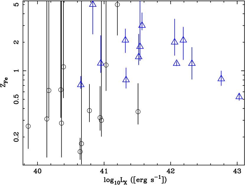
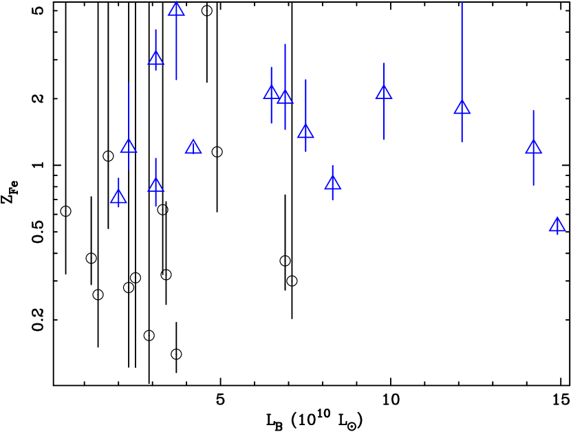
Figure 5.— Best-fitting ${\rm Z_{Fe}}$ and 1-$\sigma$ error-bars are shown as a function of ${\rm L_{X}}$ (left panel) and ${\rm L_{B}}$ (right panel). Data-points marked with a circles (black) represent those galaxies for which only a single aperture could be used, and only a single hot gas component was required by the data. The remaining galaxies are shown as triangles (blue).

6.1. Near-solar Fe abundances

In our sample of early-type galaxies, we did not find any convincing evidence for the very sub-solar ${\rm Z_{Fe}}$ historically reported for such systems. For the brighter galaxies, we found clear evidence that the ISM abundances are $\sim$solar. It is interesting to note that NGC 507 appears to be something of an “outlier” when compared to the other high-${\rm L_{X}}$ systems, since its ${\rm Z_{Fe}}$ seems to be somewhat lower than is typically seen in such objects. However, at high ${\rm L_{X}}$, the globally-averaged ${\rm Z_{Fe}}$ must start to fall in order ultimately to match ${\rm Z_{Fe}}$$\sim$0.4 typically seen in clusters, and since this is the highest-${\rm L_{X}}$ object in our sample, its lower ${\rm Z_{Fe}}$ might be expected.

Although the data for the fainter galaxies are typically of too poor quality to allow us to exclude very sub-solar abundances, they are generally consistent with ${\rm Z_{Fe}}$$\sim$1. In fact, if we consider all those systems for which only a single hot gas component was required in a single aperture (which are typically have poorer S/N), excepting the possible outlier (NGC 1553; see § 6.2), which will bias the measurement due to its small error-bars, we obtain a mean ${\rm Z_{Fe}}$=$0.58^{+0.27}_{-0.22}$. To investigate any possible correlation between ${\rm Z_{Fe}}$ and ${\rm L_{X}}$ or ${\rm L_{B}}$ we applied several statistical tests— Pearson’s linear correlation test, Spearman’s rank-order correlation test and Kendal’s $\tau$ test— to the data. In Fig 5 we show ${\rm Z_{Fe}}$ plotted against ${\rm L_{X}}$ and ${\rm L_{B}}$. Since it is possible that the S/N of the faintest galaxies masks the presence of the Fe bias, in addition to testing the correlation with the whole dataset we separately considered a subset of the galaxies, in which spatially-resolved spectroscopy or two hot gas models were required, thereby taking account of any possible Fe bias. Considering all the galaxies, Pearson’s linear correlation test did not reveal a correlation between ${\rm Z_{Fe}}$ and either ${\rm L_{X}}$ or ${\rm L_{B}}$ (${\rm p_{0}}$, the probability of no correlation, being 32% and 63%, respectively). With the non-parametric tests we found evidence of a correlation with ${\rm L_{X}}$, and marginal evidence of a correlation with ${\rm L_{B}}$ (e.g. for Spearman’s test ${\rm p_{0}}$=0.5% and 6%, respectively). Considering only the “reliable” subset of galaxies, however, all the tests failed to detect a correlation (${\rm p_{0}>20}$%), suggesting that the correlations in the entire data-set may be artefacts related to the Fe bias, although this will need to be investigated with higher-quality data. We conclude there is no convincing evidence of a correlation between ${\rm Z_{Fe}}$ and ${\rm L_{X}}$ or ${\rm L_{B}}$.

The principal reason for the under-estimate of ${\rm Z_{Fe}}$ reported in the literature appears to be overly simplistic spectral modelling, as demonstrated by Buote & Fabian (1998). In many of the fainter systems X-ray point-sources contribute $\mathrel{\hbox to0.0pt{\lower 3.0pt\hbox{$\sim$}\hss}\raise 2.0pt\hbox{$>$}}$  50% of the total X-ray flux. Using Chandra we have been able to resolve a significant fraction of these point-sources, reducing the impact of this “contaminant” and allowing less biased abundance determination. Simple fiducial models are frequently adopted to describe the spectral shape of the combined emission from undetected point-sources, but these have been by no means uniformly included in spectral-fitting in the literature. It is important to understand that these are determined empirically, and there is no a priori reason to believe them a perfect fit to the undetected source emission in any given galaxy. This issue may have been, in part, responsible for the extraordinarily low abundances reported in three low-${\rm L_{X}}$ galaxies observed with XMM by O’Sullivan & Ponman (2004), since the flux from the hot gas is most likely overwhelmed completely by the point-sources, making accurate abundance determinations very sensitive to this modelling.

With Chandra we have also been able to resolve the spatially-varying temperature structure in a number of the brighter galaxies. The excellent agreement between our measured abundances and previous single-aperture ASCA work (Buote & Fabian, 1998), where the samples overlap, confirms that the temperature gradient is sufficient to explain the multiple hot gas components required in the (large) ASCA extraction apertures. A similar conclusion was reached by Buote (1999) for a small number of bright galaxies, using Rosat, which we can now confirm with the superior spectroscopic data, and finer spatial resolution of Chandra, in a wider range of galaxies. Resolving the spatially-varying temperature structure mitigates the “Fe bias”, in which the addition of multiple components with different temperatures tends to suppress the line equivalent widths, giving artificially lower abundances. A recent dramatic example of this effect has also been seen in the Antennae galaxies (Baldi et al., 2005), where Chandra has revealed complex ISM structure in which ${\rm Z_{Fe}}$ is typically$\mathrel{\hbox to0.0pt{\lower 3.0pt\hbox{$\sim$}\hss}\raise 2.0pt\hbox{$>$}}$ 1, in contrast to previous (global) ASCA measurements of ${\rm Z_{Fe}}$$\sim$0.1.

In general, we did not require multiple hot gas components in each annulus, indicating that the ISM is not multi-phase in these regions. Although, in most cases, the presence of multiple hot gas components in the ASCA apertures can be understood in terms of a temperature gradient which we are able to resolve with Chandra, there still remains the intriguing presence of multiple hot gas components in single annuli for several of the galaxies. In most cases this is only required in the innermost bin, suggesting spatially-varying temperature structure at scales which were too small to accumulate useful spectra. In NGC 1399 and NGC 5846, however, there was some evidence that multiple temperatures may be needed over a range of annuli. In the case of NGC 5846, this simply seems to reflect the rather disturbed morphology of the galaxy. Buote (2002) first commented on the “limited multiphase gas” in NGC 1399 based on XMM data, and a similar feature is also seen in several groups (NGC 5044:Buote et al. 2003a, M 87: Gastaldello & Molendi 2002, RGH 80: Xue et al. 2004). This two-temperature structure may be related to the heating of the gas and the quenching of the cooling flow (Mathews et al., 2004).

It is worth noting that the shapes of the abundance profiles we measured are consistent with observations of the centre of the bright group NGC 5044 (Buote et al., 2003b), although we were only usually able to obtain constraints for the most massive systems, e.g. NGC 1399. Nonetheless, these abundance gradients are similar to what are predicted by the “circulation flow” model of Mathews et al. (2004) (see § 6.4).

6.2. Stellar versus ISM abundances

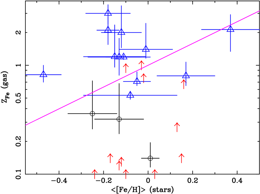
Figure 6.— A comparison of ${\rm Z_{Fe}}$ in the hot gas versus estimated mean stellar Fe abundance. We show separately the data-points for which spatially-resolved spectroscopy or multiple hot gas components were required (triangles) and those for which only a single temperature, in a single aperture was needed (circles). When no upper limit could be obtained for any galaxy, we show only the lower limit (arrows). We show the line indicating equal metallicity in both components. For clarity, any data-points lying below ${\rm Z_{Fe}}$$=0.1$ are artificially raised to this level and all error-bars shown are 1-$\sigma$.

Arimoto et al. (1997) pointed out that the historically low ISM abundances for early-type galaxies were in stark disagreement with the abundances determined for the stellar content. This is difficult to interpret in terms of simple chemical enrichment models in which the gas is enriched by stellar mass-loss and supernova ejecta. In such a scenario, we might expect the ISM abundances to exceed those in the stars (see § 6.4 for more discussion of these models). In several galaxies we found best-fitting abundances which were moderately sub-solar ($\sim$0.5), and in one case (NGC 1553) we did, in fact, obtain a best-fitting ${\rm Z_{Fe}}$ which was $\sim$0.1 (although adopting a two-temperature hot gas model, which may be more realistic in this disturbed system, the data were not inconsistent with approximately the same ISM and stellar abundances). To assess quantitatively whether there is still any evidence of the discrepancy between stellar and ISM abundances we searched the literature for optical line index measurements, from which we were able to estimate the global Fe abundances in the stars. We discuss this analysis in detail in Appendix A. Table 5 summarizes the properties of the stellar population of each galaxy.

We show a comparison of the stellar and ISM ${\rm Z_{Fe}}$ in Fig 6. The majority of the data-points cluster close to the ${\rm Z_{Fe}}$(gas)=${\rm Z_{Fe}}$(stars) line. Clearly a number of points lie significantly above this line, suggesting that these galaxies have experienced significant ISM enrichment. A few points lie slightly below the line, but are approximately consistent with it within their error-bars. Only NGC 1553 lies significantly below the line and this galaxy has a disturbed morphology, so that there is considerable uncertainty in using only one hot gas component to fit the spectrum. Alternatively, the ISM abundance for this object may in fact be low, in which case the galaxy must have acquired a substantial amount of unenriched, primordial gas. Why such a process should seem to operate so strongly only in this galaxy, and whether it is related to the disturbed morphology are not entirely clear.

If we consider those galaxies for which an upper-limit on the abundance could not be obtained, we find that the best-fitting values (not shown in Fig 6) of 4 of these systems lie above and 8 below the line. This is what we would expect if the distribution of ${\rm Z_{Fe}}$ in these systems is comparable to the “detected” galaxies. We therefore conclude that these galaxies probably have a similar Fe enrichment history, although this remains to be investigated with higher-quality data.

Based on the Chandra data, therefore, we found no evidence that the ISM abundances of the early-type galaxies in our sample (with one exception) are significantly lower than the mean metallicity of the stars. Furthermore, many of these galaxies may have ISM abundances slightly higher than the stellar component.

6.3. Supernova enrichment

Table 4Supernova enrichment fractions

Galaxy	Elements	All elements				Omitting O, S
		yield	$\chi^{2}$/dof	${\rm f^{Ia}_{gas}}$	${\rm f^{Ia}_{range}}$	yield	$\chi^{2}$/dof	${\rm f^{Ia}_{gas}}$	${\rm f^{Ia}_{range}}$
High-${\rm L_{X}}$ galaxies
IC 4296	O,Mg,Si	WDD2	$0.035/2$	$0.60\pm 0.16$	$0.28$–$1.0$	WDD2	$0.006/1$	$0.60\pm 0.16$	$0.28$–$0.63$
NGC 507	O,Ne,Mg,Si,S,Ni	W7	$16/5$	$0.67\pm 0.05$	$0.46$–$1.0$	W7	$0.95/3$	$0.70\pm 0.05$	$0.46$–$0.98$
NGC 741	O,Mg,Si,Ni	W7	$8.5/3.0$	$0.88\pm 0.05$	$0.75$–$0.91$	W7	$1.6/2$	$0.70\pm 0.13$	$0.45$–$0.94$
NGC 1132	O,Mg,Si,Ni	WDD1	$11/3$	$0.87\pm 0.07$	$0.65$–$0.87$	W7	$3.9/2$	$0.66\pm 0.12$	$0.43$–$0.77$
NGC 1399	O,Ne,Mg,Si,S,Ni	WDD2	$180/5$	$0.87\pm 0.01$	$0.70$–$0.91$	W7	$3.4/3$	$0.74\pm 0.02$	$0.49$–$1.0$
NGC 1600	O,Mg,Si	W7	$0.18/2$	$0.68^{+0.16}_{-0.21}$	$0.37$–$0.96$	W7	$0.16/1$	$0.67^{+0.16}_{-0.21}$	$0.37$–$0.75$
NGC 4472	O,Ne,Mg,Si,S,Ni	WDD1	$140/5$	$0.81\pm 0.02$	$0.53$–$0.81$	W7	$11/3$	$0.60\pm 0.03$	$0.31$–$0.66$
NGC 5846	O,Ne,Mg,Si,S,Ni	WDD2	$58/5$	$0.88\pm 0.02$	$0.71$–$0.92$	W7	$2.0/3$	$0.73\pm 0.04$	$0.49$–$0.87$
NGC 7619	O,Mg,Si,Ni	WDD2	$24/3$	$0.78\pm 0.06$	$0.49$–$0.88$	W7	$4.4/2$	$0.63\pm 0.07$	$0.27$–$0.73$
NGC 7626	Mg,Si	…	…	…	…	W7	$0.004/1$	$0.53\pm 0.29$	$0.17$–$0.59$
Moderate-${\rm L_{X}}$ galaxies
NGC 7201	O,Ne,Mg	WDD1	$21/2$	$0.85\pm 0.06$	$0.63$–$0.85$	WDD1	$2.4/1$	$0.58\pm 0.12$	$0.02$–$0.58$
NGC 13321	O,Ne,Mg,Si	WDD2	$37/3$	$0.72\pm 0.05$	$0.39$–$0.75$	W7	$2.7/2$	$0.55\pm 0.07$	$0.16$–$0.56$
NGC 1387	O,Mg,Si	W7	$0.003/2$	$0.94^{+0.06}_{-0.18}$	$0.82$–$0.94$	W7	$0.002/1$	$0.94^{+0.06}_{-0.18}$	$0.82$–$0.94$
NGC 1407	O,Mg,Si,S,Ni	WDD1	$39/4$	$0.84\pm 0.04$	$0.61$–$0.84$	W7	$1.8/2$	$0.58\pm 0.08$	$0.24$–$0.62$
NGC 1553	O,Ne	WDD2	$13/1$	$0.71\pm 0.09$	$0.33$–$0.71$	WDD1	$0/0$	$0.42\pm 0.16$	$0.0$–$0.43$
NGC 1700	O,Ne,Mg	WDD2	$3.2/2$	$0.84\pm 0.08$	$0.65$–$0.84$	WDD1	$2.3\times 10^{-7}/1$	$0.76\pm 0.11$	$0.49$–$0.76$
NGC 3607	Mg	…	…	…	…	W7	$0/0$	$0.76\pm 0.24$	$0.33$–$0.77$
NGC 3923	O,Ne,Mg,Si	WDD1	$39.1/3$	$0.89\pm 0.05$	$0.71$–$0.97$	WDD1	$5.4/2$	$0.56\pm 0.11$	$0$–$0.56$
NGC 4365	O,Mg	WDD1	$0.48/1$	$0.77^{+0.19}_{-0.27}$	$0.50$–$0.77$	WDD2	$0/0$	$0.67\pm 0.34$	$0.076$–$0.67$
NGC 4552	O,Ne,Mg,Si,Ni	WDD1	$76/4$	$0.89\pm 0.02$	$0.73$–$0.92$	W7	$3.1/3$	$0.73\pm 0.04$	$0.42$–$0.74$

Note. — The inferred SNIa enrichment fraction, ${\rm f^{Ia}_{gas}}$, for the ISM of the sample galaxies. The preferred SNIa metal yield model is listed for each galaxy (“yield”), whereas we adopt the N97 metal yields for SNII. The range of best-fitting ${\rm f^{Ia}_{gas}}$values, ${\rm f^{Ia}_{range}}$, for different combinations of SNII and SNIa yields (see text) are also shown. We show the results derived from all the measured abundance ratios (“All elements”) and those which omit, if possible, O and S, both of which seemed aberrant (see text).

With our Chandra data we have been able to obtain, in many cases for the first time, interesting constraints on $\alpha$-to-Fe abundance ratios. A number of competing effects can enrich or dilute the ISM metal content in early-type galaxies, including supernovae ejecta, stellar winds and large-scale galactic gas inflow/ outflow (Matteucci & Greggio, 1986). The $\alpha$-elements and Fe are predominantly processed through supernovae, so stellar mass-loss acts only as a “slow-release reservoir” for the elements; if the stars were all formed very quickly, we would expect the metal yields of the mass-losing stars to resemble SNII. Because these element are primarily produced in supernovae it is common-practice to define, as a fiducial diagnostic, the fraction of the Fe content of a galaxy produced in SNIa, f. Since Fe is more profusely synthesized in SNIa than SNII, typically this quantity is measured by matching linear combinations the SNe yields for a complete stellar population (integrated over an assumed IMF; typically that of Salpeter) to the abundance ratios with respect to Fe (e.g. Gastaldello & Molendi, 2002).

It is important to stress that, on account of the finite timescale over which the gas is processed through stars the SNIa fraction measured in the hot gas, ${\rm f^{Ia}_{gas}}$ and that determined from the stars, ${\rm f^{Ia}_{*}}$, are not identical, and nor are they entirely commensurate with the total fraction of Fe synthesized in SNIa during the galaxy history (Matteucci & Chiappini, 2005). However ${\rm f^{Ia}_{gas}}$ and ${\rm f^{Ia}_{*}}$ can be calibrated against realistic gasdynamical enrichment simulations (e.g. Brighenti & Mathews, 1999), making them powerful measures of the enrichment history of a galaxy; in any case, they provide a useful yard-stick with which to compare different galaxies. Furthermore the relative abundances of elements which are predominantly products of one type of supernova are fixed by the SNe yields, since there is unlikely to be significant segregation of metals produced together. This enables measurement of the abundance ratios to provide direct constraints on the SNe yields and, in principle, the IMF. Given the remarkable degree of scatter in the predicted metal yields between different explosion models (Gibson et al., 1997, hereafter G97), such constraints are of particular importance.

In order to determine values of ${\rm f^{Ia}_{gas}}$ for each galaxy we performed fitting analogous to that of Gastaldello & Molendi (2002). We experimented with different SNe metal yields, which are highly sensitive to the supernova modelling. We adopted the SNIa W7, WDD1 or WDD2 yields from Nomoto et al. (1997b) and, for ease of comparison with other authors, the SNII yields from Nomoto et al. (1997a, hereafter N97). We also experimented with a range of SNII yields taken from G97, in order to examine the sensitivity of the results to the adopted model. In practice the G97 yields are less useful than N97 since they do not all include the same range of species. It is worth noting that all of these models assume a Salpeter IMF, although the IMF is not expected to affect the abundance ratios as significantly as the overall abundances (G97). We note that fitting this model to the ${\rm Z_{O}}$/${\rm Z_{Fe}}$, ${\rm Z_{Ne}}$/${\rm Z_{Fe}}$, ${\rm Z_{Mg}}$/${\rm Z_{Fe}}$, ${\rm Z_{Si}}$/${\rm Z_{Fe}}$, ${\rm Z_{S}}$/${\rm Z_{Fe}}$and ${\rm Z_{Ni}}$/${\rm Z_{Fe}}$ ratios observed in the Sun (Asplund et al., 2004) yields the well-known ${\rm f^{Ia}_{*}}$$\sim$0.75 appropriate for the Solar neighbourhood whilst strongly favouring the WDD2 SNIa yields.

Initially we fitted our model to all of the available $\alpha$/Fe abundance ratios, adopting the SNIa model which best fitted the data. There is remarkable agreement between the supernova fractions measured in each galaxy, with ${\rm f^{Ia}_{gas}}$${\sim}$ ranging from 0.7–0.9, although it fell as low as $\sim$0.3 if the G97 yields are used. The results are summarized in Table 4. Such values are in excellent agreement with recent observations of the centres of groups and clusters. For example ${\rm f^{Ia}_{gas}}$$\sim$0.8–0.9 in M 87 (Gastaldello & Molendi, 2002), ${\rm f^{Ia}_{gas}}$$\sim$0.7–0.8 in NGC 5044 (Buote et al., 2003b) and ${\rm f^{Ia}_{gas}}$$\sim$0.8–0.9 in the centre of the cluster A 1795 (Ettori et al., 2002). We found a general trend that the delayed detonation SNIa yields were preferred over the deflagration (W7) model, although this seems to be driven by the low ${\rm Z_{O}}$/${\rm Z_{Mg}}$ ratios in these models, which could be a source of uncertainty (see below).

In contrast to the enrichment of the gas, super-solar $\alpha/Fe$ ratios are typically reported in the stars when simple stellar population models are fitted (see Appendix A), which implies substantially more Type II enrichment in the stars. Assuming the $\alpha/Fe$ abundances obtained in Table 5 are driven primarily by the Mg/Fe ratio (and assuming that there is no stellar Mg/Fe gradient), we estimate an average ${\rm f^{Ia}_{*}}$${\sim 0.35}$, with individual values ranging from $\sim 0.60$ for NGC 5018 to $\sim 0.1$ for NGC 1399, adopting the W7 SNIa and N97 SNII yields. This is a well-known result (e.g. Worthey, 1998) which is typically explained in terms of the short timescale of star-formation in early-type galaxies, or variations in the IMF. The stark discrepancy between ${\rm f^{Ia}_{gas}}$ and ${\rm f^{Ia}_{*}}$ can readily be explained only if substantial amounts of Fe are added to the ISM through SNIa occurring after the bulk of the stars have formed. Such a large input of Fe into the ISM would tend to raise ${\rm Z_{Fe}}$ to $\sim$2–3 times the mean stellar value. The error-bars on our measured ${\rm Z_{Fe}}$ in the gas are sufficiently large that many of the galaxies in the sample could have ${\rm Z_{Fe}}$consistent with such an elevated value; in particular we note that NGC 1332 and NGC 4472 have best-fit abundances close to that required by this argument. However, several galaxies (most notably NGC 1399 and NGC 720) seem to have ${\rm Z_{Fe}}$ about a factor $\sim$2 too low, implying dilution of the ISM by a source of primordial (i.e. un-enriched) gas in these systems.

Despite consistency with ${\rm f^{Ia}_{gas}}$ determined in other systems, it is clear that the fits are typically rather poor, suggesting a disagreement between the standard SNe yields and the ISM abundance pattern. This primarily arises because of discrepant $\alpha$-element abundance ratios, even taking into account the large scatter in the SNII yields. The chiefly discrepant species is O, which appears to be significantly under-abundant in comparison to other $\alpha$-elements, such as Mg (for which we have the most measurements). The measurement of reliable ${\rm Z_{O}}$ in the X-ray band is challenging, especially when attempting imaging spectroscopy at energies where the CCD response may not be perfectly well understood (§ 5). At plasma temperatures $\sim$0.5–1.0 keV, appropriate for our sample, the principal O features tend to be blended somewhat with the Fe L-shell “hump” which exacerbates the difficulty in reliably determining ${\rm Z_{O}}$. However, unexpectedly low values of ${\rm Z_{O}}$/${\rm Z_{Mg}}$ ($\sim$0.8–1.3, given our default solar abundances) have been widely reported in the literature, in contrast to ${\rm Z_{O}}$/${\rm Z_{Mg}}$$\sim$1.4–2.8 predicted by SNII models (G97). This discrepancy has been found in both imaging and grating spectroscopy data from a variety of different instruments observing a wide range of systems such as the bright group NGC 5044 (Buote et al., 2003b; Tamura et al., 2003), M 87 (Gastaldello & Molendi, 2002; Sakelliou et al., 2002), the massive elliptical NGC 4636 (Xu et al., 2002), the starbursting galaxy M 82 (Tsuru et al., 1997) and the centres of some galaxy clusters (Peterson et al., 2003). There is even some evidence of this effect in the Milky Way ISM (Ueda et al., 2005).

It is not certain whether the observed O deficiency represents a problem with the SN yields, which are highly sensitive to the (rather uncertain) SNe modelling (G97), or if it is indicative of an additional source of metal enrichment within the galaxy. It is interesting to note that some SNR have been observed with apparent abundance anomalies (for example N49B in which the ejecta appear significantly enriched in Mg without accompanying Ne or O: Park et al. 2003), which might hint at a problem with the nuclear physics. In contrast, Loewenstein (2001) suggested there may be an alternative source of metal enrichment to explain the low ${\rm Z_{O}}$/${\rm Z_{Fe}}$ in clusters. He proposed that significant enrichment in the early universe may arise from population III hypernovae, since the O-burning region is significantly expanded in an hypernova. Hypernova metal yields have been computed by Umeda et al. (2002) and Heger & Woosley (2002), but unfortunately they did not exhibit the very low ${\rm Z_{O}}$/${\rm Z_{Mg}}$ (nor ${\rm Z_{O}}$/${\rm Z_{Ne}}$) which are observed in our data, although the calculations for Mg and Ne production are sensitive to the model assumptions. Given the published Pop III hypernova yields Matteucci & Pipino (2005) pointed out they would not have a significant impact upon the abundance pattern of an elliptical galaxy.

Given these reservations, we did not attempt to include a putative hypernova component in our modelling. If, instead, the discrepancy between the observed and predicted abundance of O reflects a problem in the computed yields, notwithstanding their success in reproducing the Solar abundance pattern, an alternative approach is simply to omit this element from the computation of ${\rm f^{Ia}_{gas}}$. This tended to result in slightly lower estimated values of ${\rm f^{Ia}_{gas}}$, but substantially improved $\chi^{2}$. Interestingly we also found that ${\rm Z_{S}}$/${\rm Z_{Fe}}$, where it could be measured, was slightly under-predicted by the model (which may be a systematic error; § 5.1) and so we also omitted this element, although it had little impact on the best-fitting ${\rm f^{Ia}_{gas}}$. The fit results are shown in Table 4. We found a mean ${\rm f^{Ia}_{gas}}$=$0.66\pm 0.11$, where the quoted error is the standard deviation in the measurements. Using the same statistical tests described in § 6.1 we searched for correlations between ${\rm f^{Ia}_{gas}}$ and ${\rm L_{X}}$, ${\rm L_{B}}$ and ${\rm Z_{Fe}}$, but found no evidence of any such correlations (${\rm p_{0}>40}$% in all cases). In this case, we found that the W7 (deflagration model) abundance yields are preferred over the delayed detonation models, although in most cases (with one or two notable exceptions, such as NGC 1399) the data do not strongly discriminate between them. It is striking that ${\rm f^{Ia}_{gas}}$ in these galaxies is remarkably similar to that in the Solar neighbourhood, implying a similar enrichment history for the hot ISM of early-type galaxies and the cold ISM of spirals.

An intriguing piece of evidence which further complicates this picture of metal enrichment is the observation that [O/Mg] in Galactic bulge stars appears to be a decreasing function of metallicity (Fulbright et al., 2004). There is a reduction in [O/Mg] by as much as $\sim$0.5 dex with respect to the SN II yield level by ${\rm Z_{Fe}}$$\sim$1, providing evidence that O may be under-abundant in old stellar populations, not just the ISM. Moreover such a trend is very difficult to reconcile with a picture where only SNII and SNIa enrich the gas. Nonetheless whether a putative Pop III hypernova population could resolve this issue is unclear.

6.4. Enrichment models

We now discuss our results in the light of various models for the chemical enrichment of early-type galaxies. In traditional “galactic wind models” the galaxies form monolithically and passively evolve, during which time the dynamics and luminosity of the gas is strongly affected by supernova feedback, which can drive periods of large scale galactic outflow (e.g. Ciotti et al., 1991). Given the large amount of metals injected into the ISM by the supernovae, these models tend to predict ${\rm Z_{Fe}}$$\sim$a few times solar, (and, certainly, dramatically in excess of the abundance of the stars), which is clearly in disagreement with the majority of galaxies in the sample, in many cases by as much as an order of magnitude. Pipino et al. (2005) allowed the accretion of additional, unenriched gas, but were unable to mitigate this discrepancy while reproducing the other optical and X-ray properties of the gas. In contrast, Brighenti & Mathews (1999) constructed a cooling-flow gasdynamical model for NGC 4472, incorporating the prolonged infall of gas. These authors were able to produce $\sim$0.5 solar abundances for the galaxy (the precise abundances being rather sensitive to the assumed supernovae rates), although the density profile was too peaked on account of excessive cooling in the core. Furthermore, the enrichment history assumed in this model makes it difficult to understand the large amount of metals in clusters in terms of the contribution from elliptical galaxies.

An alternative approach was adopted by Kawata & Gibson (2003), who followed the evolution of a $\sim 10^{13}$${\rm M_{\odot}}$ elliptical galaxy in an hierarchical structure formation simulation. In their model, however, most of the Fe produced by the stars is locked into large amounts of cool ($\sim 10^{4}$ K) gas and excessive on-going star formation, at variance with observations. In this case the hot phase ISM was found to have ${\rm Z_{Fe}}$$\mathrel{\hbox to0.0pt{\lower 3.0pt\hbox{$\sim$}\hss}\raise 2.0pt\hbox{$<$}}$ 0.3 and, critically ${\rm Z_{Fe}}$(stars) was $\sim$an order of magnitude greater than that of the hot gas. The results are clearly at variance with our Chandra measurements, in the opposite sense to the galactic wind models.

One key ingredient not typically incorporated into enrichment models is the role of AGN feedback. There is some evidence of disturbances in some “normal” early-type galaxies which may point to interaction between the ubiquitous supermassive central black-hole and the ISM (e.g. Blanton et al., 2001; Jones et al., 2002). Numerical simulations have suggested that ISM-AGN interactions can have a dramatic effect on the dynamics and energetics of the ISM (Di Matteo et al., 2005). Kawata & Gibson (2005) incorporated AGN feedback into their model, finding that this effectively evacuated the (cool) enriched gas from the galaxy, so that the discrepancy between stellar and ISM abundances of their model persists. We note that these authors comment on the good agreement between their model and ${\rm Z_{Fe}}$ for the galaxy NGC 3923, based on the results of Matsushita et al. (2000). Our analysis of the Chandra data indicates a significantly higher abundance for this galaxy, underlining the discrepancy between our results and the predictions of this model. Mathews et al. (2004), in contrast, showed that allowing a small amount of continuous heating from a central AGN may drive large-scale “circulation flows”, which efficiently mixes gas through the galaxy. This model could reproduce the abundance gradients found in the XMM and Chandra data of the group NGC 5044. Crucially it predicted the correct ${\rm Z_{Fe}}$, which is coincidentally similar to that observed in most galaxies in our sample. Whether a variant of this model can successfully describe the lower-mass systems studied in this present work remains to be seen, however.

7. Summary

We have surveyed the metal abundances of the hot phase ISM within a sample of 28 early-type galaxies, using Chandra. In summary:

1. We did not find the historically very sub-solar abundances reported for early-type galaxies, nor is there convincing evidence that ${\rm Z_{Fe}}$ correlates with the galaxy luminosity. Considering just our lowest-S/N galaxies, we found a mean ${\rm Z_{Fe}}$=0.58${}^{+0.27}_{-0.22}$. The discrepancy with past results appears to be due to imperfect modelling of the (undetected) point-source populations (of which Chandra has enabled a substantial fraction to be detected) and the fitting of single-temperature models to multi-temperature gas (the Fe bias).

2. We confirmed the conclusions of Buote & Fabian (1998) that multiple components are often required to fit the spectra of early-type galaxies. In a number of cases the excellent spatial resolution of Chandra enabled us to resolve temperature gradients lying within ASCA or Rosat spectral extraction apertures. In a few cases the fit required multiple hot gas components in a given annulus. In all cases a component was required to account for undetected point-sources.

3. Comparing the emission-weighted ISM and stellar Fe abundances we found excellent agreement. Excepting one possible outlier (NGC 1553) there is no evidence that the stellar abundances are significantly higher than those of the gas. In fact the data allow the ISM ${\rm Z_{Fe}}$ to be slightly higher on average.

4. The data are inconsistent with both monolithic “galactic wind models”, which over-predict ${\rm Z_{Fe}}$ and the recent hierarchical models of Kawata & Gibson (2005), which under-predict ${\rm Z_{Fe}}$. The “circulation flow” model of Mathews et al. (2004) is able to explain ${\rm Z_{Fe}}$ of about the correct magnitude, albeit for a system more massive than most considered here.

5. We found that the SNIa Fe enrichment fraction in the hot gas, ${\rm f^{Ia}_{gas}}$, is $66\pm 11$% and shows no obvious trend with luminosity. This value is remarkably close to the 75% enrichment fraction for the solar neighbourhood, indicating similarity in the enrichment histories for the early-type and spiral galaxies. It is also similar to that observed in the centres of clusters and groups, indicating homology of enrichment from cluster scales to intermediate-${\rm L_{X}}$ galaxies.

6. The ${\rm Z_{Mg}}$/${\rm Z_{Fe}}$ ratio in the gas is significantly lower than that in the stars, indicating that significant SNIa must enrich the gas, in addition to stellar mass-loss. In at least two cases (NGC 1399 and NGC 720) this would seem to require the further accretion of unenriched, “primordial” material to prevent ${\rm Z_{Fe}}$ being significantly higher than observed.

7. There is increasing evidence that O is over-predicted by the SNII yields, which may imply problems in the supernova calculations. Alternatively, the measurement of varying [O/Mg] in Galactic bulge stars may point to a source of $\alpha$-element enrichment in addition to SNIa and SNII.

Appendix A Stellar abundance estimates

In order to estimate the mean Fe abundance in the stars, we searched the literature to obtain reliable Lick/IDS index (Faber et al., 1985) measurements for the centre of each galaxy. In order to break the age-metallicity degeneracy, we converted the line indices into ${\rm[Fe/H]}$ by linearly interpolating the simple stellar population (SSP) model results of Thomas et al. (2003). These models take into account non-solar $\alpha$-element to Fe ratios, which are typically reported in early-type galaxies (e.g. Trager et al., 2000). Where possible, we fitted the interpolated model with a $\chi^{2}$ minimization procedure to the central H$\beta$, Mgb, Fe5270 and Fe5335 indices. In several cases some or all of these indices were not available in the literature, in which case we either adopted appropriate alternative indices or omitted them. In a number of cases one or more of the indices appeared to be discrepant with the others, which may be a consequence of systematic measurement errors (or, possibly, the breakdown of the SSP model assumptions). In these cases, we omitted the most discrepant index. In Table 5 we list the indices used for each galaxy. For NGC 1387, we could not find useful line index measurements in the literature, and so we omitted it from the comparison with the X-ray results (§ 6.2). For several galaxies, it was necessary to fix the age or [$\alpha$/Fe] in order to obtain interesting abundance constraints. In these cases, we adopted an age of 12 Gyr and [$\alpha$/Fe]=0.23, which are roughly consistent with the average values found in the remaining galaxies. The best-fitting parameter values, converted to the solar abundances standard of Asplund et al. (2004), and the reference from which the line strength measurements were derived are shown in Table 5.

It is interesting to compare our results with those of other recent catalogues of ages and metal abundances in early-type galaxies which overlap with our sample. Thomas et al. (2005) measured ages and central abundances for a sample of galaxies, of which 14 overlapped our sample, using the SSP models adopted in this present work. In general we found good agreement with our results; the only two galaxies for which ${\rm Z_{Fe}}$ was substantially discrepant were NGC 1600 and NGC 7619, for which our abundances were $\sim$0.1 dex higher. Terlevich & Forbes (2002) and Trager et al. (2000) both estimated (central) metal abundances, ages and $\alpha$/Fe ratios using the older SSP models of Worthey (1994). Trager et al. (2000) made corrections for non-solar $\alpha$/Fe ratios so that [Fe/H] could explicitly be obtained. In contrast, Terlevich & Forbes (2002) adopted the [MgFe] lick index, which is more sensitive to the overall abundance (${\rm[Z/H]=[Fe/H]+0.94[\alpha/Fe]}$ for the models we adopt). In general our results agree reasonably well ($\pm 2\sigma$) with these previous measurements where the data overlap. There was some scatter, however; for example we found that our central [Fe/H] were typically $\sim$0.1 dex higher than those found by Trager et al. (2000). We found the most significant discrepancies ($\mathrel{\hbox to0.0pt{\lower 3.0pt\hbox{$\sim$}\hss}\raise 2.0pt\hbox{$>$}}$ 3$\sigma$) between our results and those of Terlevich & Forbes (2002) for the galaxies NGC 1553, NGC 3115 and NGC 3607, for all of which those authors reported poor quality data. Given the good agreement with Thomas et al. (2005), the differences are likely a consequence of the different SSP models used.

To estimate the total Fe content of the stars it is necessary to take into account any abundance gradients. There is a substantial body of literature on line index gradients in early-type galaxies (see Kobayashi & Arimoto, 1999, and references therein). Probably the most extensive collection of abundance gradient measurements in early-type galaxies overlapping our sample is that of Kobayashi & Arimoto (1999) who used linear approximations for the line-strength–metallicity relations at fixed galaxy ages and treated each line index separately. Unfortunately, their results were very sensitive to the line index adopted, and their method for relaxing the age constraint was not always successful for each galaxy (see their results for NGC 720). A fully self-consistent assessment of stellar abundance gradients in all of our galaxies is beyond the scope of this present work. However, for those galaxies in the sample of Trager et al. (2000), we fitted simultaneously the data in both the ${\rm r_{e}/8}$ and ${\rm r_{e}/2}$ apertures (where ${\rm r_{e}}$ is the effective radius of the galaxy), assuming that the age and $\alpha$/Fe ratios are the same in each aperture. This allowed us to estimate the magnitude of the stellar abundance gradient. We note that Trager et al. (2000) allowed for both age and $\alpha$/Fe ratio gradients, but we typically did not find this necessary to obtain good fits. In any case, if the overall stellar population comprises a mixture of different-aged components, the application of single burst SSP models is probably overly simplistic. To estimate the global emission-weighted Fe abundance, we adopted the prescription of Arimoto et al. (1997), who assumed ${\rm Z_{Fe}}$${\rm\propto r^{-c}}$ for the stars, where r is the distance from the galactic centre. Assuming a circular aperture, which is appropriate for these line index measurements (see González, 1993), and a de Vaucouleurs optical brightness profile, we can express the emission weighted abundance within aperture r as:

$$\bar{{Z}_{Fe}}(r)=\bar{{Z}_{Fe}}(\infty)\frac{P(8-4c,7.67(r/r_{e})^{1/4})}{P(8,7.67(r/r_{e})^{1/4})}$$

where $P(a,x)$ is the incomplete gamma function $\int_{0}^{x}dt\ \exp(-t)t^{a-1}/\Gamma(a)$. Two abundance measurements in different apertures are therefore sufficient to constrain both unknowns, c and $\bar{{Z}_{Fe}}(\infty)$, of which the latter is the quantity of interest for comparison with the X-ray results. Following convention, we henceforth denote ${\rm\log_{10}(\bar{Z_{Fe}}(r_{e}/8))\equiv[Fe/H]_{0}}$ and ${\rm\log_{10}(\bar{Z_{Fe}}(\infty))\equiv<[Fe/H]>}$. For the 10 of our galaxies in the Trager et al. (2000) sample, we found that the weighted mean of the difference between ${\rm<[Fe/H]>}$ and [Fe/H]₀ was $-0.27\pm 0.06$. This corresponds to c=0.24, in good agreement with the average $\sim$0.3 found by Kobayashi & Arimoto (1999). Therefore, we used this factor to estimate the global abundances where we only had central line indices. The assumed power law relation for ${\rm Z_{Fe}}$ must break down at small radii, since it inflates unphysically, and so, for convenience, we assume that any “central” abundances inferred from the literature are the same as would be measured in an ${\rm r_{e}/8}$ aperture. In practice correcting from an aperture of size ${\rm r_{e}/10}$ to one of size ${\rm r_{e}/8}$ involves shifting the abundances only by 0.02 dex, which is considerably smaller than the statistical errors.

Table 5Stellar population parameters

Galaxy	indices	ref.	${\rm[\alpha/Fe]}$	age	${\rm[Fe/H]_{0}}$	$\rm<[Fe/H]>$
				(Gyr)
IC 4296	Mg2, Mgb, Fe5270, Fe5335	2	0.31$\pm 0.08$	12	0.12$\pm$0.10	-0.10$\pm$0.11‡
NGC 507	H$\beta$, Mgb, Fe5270, Fe5335	4	0.30$\pm 0.05$	7.0$\pm 3.0$	0.00$\pm$0.11	-0.08$\pm$0.35
NGC 720	H$\beta$, Mgb, Fe5270, Fe5335	4	0.37$\pm 0.05$	2.9${}^{+1.3}_{-0.3}$	0.30$\pm$0.14	0.17$\pm$0.21
NGC 741	H$\beta$, Mgb, Fe5270, Fe5335	5	0.20$\pm 0.16$	12	0.09$\pm$0.22	-0.13$\pm$0.23‡
NGC 1132	Mg2	3	0.23	12	-0.25$\pm$0.11	-0.47$\pm$0.13‡
NGC 1332	H$\beta$, Mgb, Fe5270, Fe5335	5	0.31$\pm 0.16$	12	0.07$\pm$0.22	-0.15$\pm$0.23‡
NGC 1399	H$\beta$, Mgb, Fe5270, Fe5335	1	0.37$\pm 0.05$	12${}^{+4}_{-3}$	0.11$\pm 0.11$	-0.11$\pm 0.13$‡
NGC 1407	H$\beta$, Mgb, Fe5270, Fe5335	1	0.33$\pm 0.02$	12$\pm 2$	0.04$\pm 0.06$	-0.18$\pm 0.08$‡
NGC 1549	H$\beta$, Mgb, Fe5270, Fe5335	1	0.24$\pm 0.01$	5.1$\pm 0.7$	0.12$\pm 0.03$	-0.10$\pm 0.07$‡
NGC 1553	H$\beta$, Mgb, Fe5270, Fe5335	1	0.17$\pm 0.01$	5.7${}^{+1.2}_{-0.8}$	0.23$\pm$0.04	0.01$\pm$0.07‡
NGC 1600	H$\beta$, Mgb, Fe5335	4	0.24$\pm 0.02$	6.6$\pm 2.3$	0.30$\pm$0.07	0.37$\pm 0.21$
NGC 1700	H$\beta$, Mgb, Fe5270, Fe5335	4	0.16$\pm 0.02$	2.8${}^{+0.5}_{-0.4}$	0.31$\pm$0.08	0.16$\pm$0.12
NGC 3115	H$\beta$, Mgb, Fe5270, Fe5335	5	0.11$\pm 0.11$	12	0.25$\pm 0.16$	0.03$\pm 0.17$‡
NGC 3585	H$\beta$, Mgb, Fe5270, Fe5335	5	0.20$\pm 0.12$	12	0.09$\pm$0.17	-0.13$\pm$0.18‡
NGC 3607	H$\beta$, Mgb, Fe5270, Fe5335	5	0.19$\pm 0.12$	15$\pm 4$	0.09$\pm$0.17	-0.13$\pm$0.18‡
NGC 3608	H$\beta$, Mgb, Fe5270, Fe5335	4	0.19$\pm 0.03$	8.2$\pm 2.0$	0.16$\pm$0.07	-0.17$\pm$0.16
NGC 3923	H$\beta$, Mgb, Fe5270, Fe5335	1	0.34$\pm$0.03	3.3${}^{+0.7}_{-0.3}$	0.35$\pm$0.08	0.13$\pm$0.10‡
NGC 4365	H$\beta$, Mgb, Fe5270, Fe5335	5	0.19$\pm$0.14	12	0.20$\pm$0.18	-0.02$\pm$0.19‡
NGC 4472	H$\beta$, Mgb, Fe5270, Fe5335	4	0.25$\pm 0.03$	9.0$\pm 2.0$	0.13$\pm 0.06$	-0.01$\pm 0.20$
NGC 4494	H$\beta$, Mgb, Fe5270, Fe5335	5	0.16$\pm 0.13$	12	-0.02$\pm$0.19	-0.24$\pm$0.19‡
NGC 4552	H$\beta$, Mgb, Fe5335	4	0.24$\pm 0.02$	12$\pm 1.7$	0.17$\pm 0.04$	-0.05$\pm$0.10
NGC 4621	H$\beta$, Mgb, Fe5335	5	0.28$\pm$0.14	12	0.19$\pm$0.17	-0.03$\pm$0.18‡
NGC 5018	H$\beta$, Mgb, Fe5335	5	0.01$\pm$0.14	2.0${}^{+2.3}_{-0.4}$	0.37$\pm$0.27	0.15$\pm$0.28‡
NGC 5845	H$\beta$, Mgb, Fe5335	5	0.26$\pm$0.17	12	0.10$\pm$0.25	-0.12$\pm$0.26‡
NGC 5846	H$\beta$, Mgb, Fe5335	4	0.22$\pm 0.02$	15$\pm$2.0	0.05$\pm 0.04$	-0.18$\pm 0.16$
NGC 7619	H$\beta$, Mgb, Fe5335	4	0.18$\pm 0.02$	13.5$\pm 1.0$	0.21$\pm 0.04$	-0.12$\pm 0.15$
NGC 7626	H$\beta$, Mgb, Fe5335	4	0.24$\pm 0.02$	14$\pm 2$	0.08$\pm 0.05$	-0.25$\pm 0.18$

Note. — The mean abundances determined from fitting SSP models to the Lick indices reported in the literature. Those mean stellar abundances (${\rm<[Fe/H]>}$) marked ‡ were estimated from the central abundance (${\rm[Fe/H]_{0}}$) assuming a constant abundance gradient; otherwise the mean abundance is inferred by extrapolation (see text). Where no error-bar is given, the parameter was frozen. Table references: 1— Beuing et al. (2002), 2— Gorgas et al. (1990), 3— LEDA  4— Trager et al. (2000), 5— Trager et al. (1998)

References

- Anders & Grevesse (1989) Anders, E. & Grevesse, N. 1989, Geochim. Cosmochim. Acta, 53, 197
- Arimoto et al. (1997) Arimoto, N., Matsushita, K., Ishimaru, Y., Ohashi, T., & Renzini, A. 1997, ApJ, 477, 128
- Asplund et al. (2004) Asplund, M., Grevesse, N., & Sauval, J. 2004, in Cosmic abundances as records of stellar evolution and nucleosynthesis, ed. F. N. Bash & T. G. Barnes (ASP Conf. series), astro-ph/0410214
- Baldi et al. (2005) Baldi, A., Raymond, H. C., Fabbiano, G., Zezas, A., Rots, A. H., Schweizer, F., King, A. R., & Ponman, T. J. 2005, ApJS, in press, astro-ph/0410192
- Behar et al. (2001) Behar, E., Cottam, J., & Kahn, S. M. 2001, ApJ, 548, 966
- Beuing et al. (2002) Beuing, J., Bender, R., Mendes de Oliveira, C., Thomas, D., & Maraston, C. 2002, A&A, 395, 431
- Blanton et al. (2001) Blanton, E. L., Sarazin, C. L., & Irwin, J. A. 2001, ApJ, 552, 106
- Brighenti & Mathews (1999) Brighenti, F. & Mathews, W. G. 1999, ApJ, 515, 542
- Buote (1999) Buote, D. A. 1999, MNRAS, 309, 685
- Buote (2000a) Buote, D. A. 2000a, ApJ, 539, 172
- Buote (2000b) Buote, D. A. 2000b, MNRAS, 311, 176
- Buote (2002) Buote, D. A. 2002, ApJ, 574, L135
- Buote et al. (2004) Buote, D. A., Brighenti, F., & Mathews, W. G. 2004, ApJ, 607, L91
- Buote & Canizares (1994) Buote, D. A. & Canizares, C. R. 1994, ApJ, 427, 86
- Buote & Fabian (1998) Buote, D. A. & Fabian, A. C. 1998, MNRAS, 296, 977
- Buote et al. (2003a) Buote, D. A., Lewis, A. D., Brighenti, F., & Mathews, W. G. 2003a, ApJ, 594, 741
- Buote et al. (2003b) Buote, D. A., Lewis, A. D., Brighenti, F., & Mathews, W. G. 2003b, ApJ, 595, 151
- Church & Bałucińska-Church (2001) Church, M. J. & Bałucińska-Church, M. 2001, A&A, 369, 915
- Ciotti et al. (1991) Ciotti, L., Pellegrini, S., Renzini, A., & D’Ercole, A. 1991, ApJ, 376, 380
- Davis & White (1996) Davis, D. S. & White, R. E. 1996, ApJ, 470, L35
- Di Matteo et al. (2005) Di Matteo, T., Springel, V., & Hernquist, L. 2005, Nature, 433, 604
- Dickey & Lockman (1990) Dickey, J. M. & Lockman, F. J. 1990, ARA&A, 28, 215
- Ettori et al. (2002) Ettori, S., Fabian, A. C., Allen, S. W., & Johnstone, R. M. 2002, MNRAS, 331, 635
- Fabbiano et al. (1994) Fabbiano, G., Kim, D.-W., & Trinchieri, G. 1994, ApJ, 429, 94
- Faber et al. (1985) Faber, S. M., Friel, E. D., Burstein, D., & Gaskell, C. M. 1985, ApJS, 57, 711
- Faber et al. (1989) Faber, S. M., Wegner, G., Burstein, D., Davies, R. L., Dressler, A., Lynden-Bell, D., & Terlevich, R. J. 1989, ApJS, 69, 763
- Finoguenov & Jones (2000) Finoguenov, A. & Jones, C. 2000, ApJ, 539, 603
- Freeman et al. (2002) Freeman, P. E., Kashyap, V., Rosner, R., & Lamb, D. Q. 2002, ApJS, 138, 185
- Fulbright et al. (2004) Fulbright, J. P., Rich, R. M., & McWilliam, A. 2004, in Nuclei in the Cosmos VIII, Vancouver, BC, July 2004
- Gastaldello et al. (2004) Gastaldello, F., Buote, D. A., Mathews, W., & Brighenti, F. 2004, in 8th Meeting of the AAS High Energy Astrophysics Division, 8–11 Sept, 2004, New Orleans, LA
- Gastaldello & Molendi (2002) Gastaldello, F. & Molendi, S. 2002, ApJ, 572, 160
- Gibson et al. (1997) Gibson, B. K., Loewenstein, M., & Mushotzky, R. F. 1997, MNRAS, 290, 623
- González (1993) González, J. J. 1993, Ph.D. Thesis, University of California, Santa Cruz
- Gorgas et al. (1990) Gorgas, J., Efstathiou, G., & Salamanca, A. A. 1990, MNRAS, 245, 217
- Grevesse & Sauval (1998) Grevesse, N. & Sauval, A. J. 1998, Space Science Reviews, 85, 161
- Heger & Woosley (2002) Heger, A. & Woosley, S. E. 2002, ApJ, 567, 532
- Humphrey & Buote (2004) Humphrey, P. J. & Buote, D. A. 2004, ApJ, 612, 848
- Humphrey et al. (2004) Humphrey, P. J., Buote, D. A., & Canizares, C. R. 2004, ApJ, 617, 1047
- Irwin et al. (2003) Irwin, J. A., Athey, A. E., & Bregman, J. N. 2003, ApJ, 587, 356
- Irwin et al. (2002) Irwin, J. A., Sarazin, C. L., & Bregman, J. N. 2002, ApJ, 570, 152
- Jensen et al. (2003) Jensen, J. B., Tonry, J. L., Barris, B. J., Thompson, R. I., Liu, M. C., Rieke, M. J., Ajhar, E. A., & Blakeslee, J. P. 2003, ApJ, 583, 712
- Jones et al. (2002) Jones, C., Forman, W., Vikhlinin, A., Markevitch, M., David, L., Warmflash, A., Murray, S., & Nulsen, P. E. J. 2002, ApJ, 567, L115
- Jones et al. (1997) Jones, C., Stern, C., Forman, W., Breen, J., David, L., Tucker, W., & Franx, M. 1997, ApJ, 482, 143
- Kawata & Gibson (2003) Kawata, D. & Gibson, B. K. 2003, MNRAS, 346, 135
- Kawata & Gibson (2005) Kawata, D. & Gibson, B. K. 2005, MNRAS, 358, L16
- Kim & Fabbiano (2003) Kim, D. & Fabbiano, G. 2003, ApJ, 586, 826
- Kim & Fabbiano (2004a) Kim, D. & Fabbiano, G. 2004a, ApJ, 611, 846
- Kim & Fabbiano (2004b) Kim, D. & Fabbiano, G. 2004b, ApJ, 613, 933
- Kim et al. (1996) Kim, D.-W., Fabbiano, G., Matsumoto, H., Koyama, K., & Trinchieri, G. 1996, ApJ, 468, 175
- Kobayashi & Arimoto (1999) Kobayashi, C. & Arimoto, N. 1999, ApJ, 527, 573
- Kraft et al. (2004) Kraft, R. P., Forman, W. R., Churazov, E., Laslo, N., Jones, C., Markevitch, M., Murray, S. S., & Vikhlinin, A. 2004, ApJ, 601, 221
- Loewenstein (2001) Loewenstein, M. 2001, ApJ, 557, 573
- Loewenstein & Mathews (1991) Loewenstein, M. & Mathews, W. G. 1991, ApJ, 373, 445
- Loewenstein & Mushotzky (1998) Loewenstein, M. & Mushotzky, R. F. 1998, in IAU Symp. 188: The Hot Universe, 53
- Markevitch (2002) Markevitch, M. 2002, astro-ph/0205333
- Mathews & Brighenti (2003) Mathews, W. G. & Brighenti, F. 2003, ARA&A, 41, 191
- Mathews et al. (2004) Mathews, W. G., Brighenti, F., & Buote, D. A. 2004, ApJ, 615, 662
- Matsushita et al. (2000) Matsushita, K., Ohashi, T., & Makishima, K. 2000, PASJ, 52, 685
- Matsushita et al. (1994) Matsushita, K., et al. 1994, ApJ, 436, L41
- Matteucci & Chiappini (2005) Matteucci, F. & Chiappini, C. 2005, Publications of the Astronomical Society of Australia, 22, 49
- Matteucci & Greggio (1986) Matteucci, F. & Greggio, L. 1986, A&A, 154, 279
- Matteucci & Pipino (2005) Matteucci, F. & Pipino, A. 2005, MNRAS, 64
- Mulchaey et al. (2003) Mulchaey, J. S., Davis, D. S., Mushotzky, R. F., & Burstein, D. 2003, ApJS, 145, 39
- Mulchaey & Zabludoff (1999) Mulchaey, J. S. & Zabludoff, A. I. 1999, ApJ, 514, 133
- Nomoto et al. (1997a) Nomoto, K., Hashimoto, M., & Tsujimoto, T. 1997a, Nucl. Phys. A, 616, 79
- Nomoto et al. (1997b) Nomoto, K., Iwamoto, K., Nakasoto, N., Thielemann, F. K., Brachwitz, F., Tsujimoto, T., Kubo, Y., & Kishimoto, N. 1997b, Nucl. Phys. A, 621, 467
- O’Sullivan et al. (2001) O’Sullivan, E., Forbes, D. A., & Ponman, T. J. 2001, MNRAS, 328, 461
- O’Sullivan & Ponman (2004) O’Sullivan, E. & Ponman, T. J. 2004, MNRAS, 349, 535
- O’Sullivan et al. (2003) O’Sullivan, E., Vrtilek, J. M., Read, A. M., David, L. P., & Ponman, T. J. 2003, MNRAS, 346, 525
- Park et al. (2003) Park, S., Hughes, J. P., Slane, P. O., Burrows, D. N., Warren, J. S., Garmire, G. P., & Nousek, J. A. 2003, ApJ, 592, L41
- Peterson et al. (2003) Peterson, J. R., Kahn, S. M., Paerels, F. B. S., Kaastra, J. S., Tamura, T., Bleeker, J. A. M., Ferrigno, C., & Jernigan, J. G. 2003, ApJ, 590, 207
- Pipino et al. (2005) Pipino, A., Kawata, D., Gibson, B. K., & Matteucci, F. 2005, A&A, 434, 553
- Renzini (1997) Renzini, A. 1997, ApJ, 488, 35
- Sakelliou et al. (2002) Sakelliou, I., et al. 2002, A&A, 391, 903
- Sambruna et al. (2004) Sambruna, R. M., Gliozzi, M., Donato, D., Tavecchio, F., Cheung, C. C., & Mushotzky, R. F. 2004, A&A, 414, 885
- Sarazin et al. (2001) Sarazin, C. L., Irwin, J. A., & Bregman, J. N. 2001, ApJ, 556, 533
- Sivakoff et al. (2004) Sivakoff, G. R., Sarazin, C. L., & Carlin, J. L. 2004, ApJ, 617, 262
- Sivakoff et al. (2003) Sivakoff, G. R., Sarazin, C. L., & Irwin, J. A. 2003, ApJ, 599, 218
- Statler & McNamara (2002) Statler, T. S. & McNamara, B. R. 2002, ApJ, 581, 1032
- Tamura et al. (2003) Tamura, T., Kaastra, J. S., Makishima, K., & Takahashi, I. 2003, A&A, 399, 497
- Terlevich & Forbes (2002) Terlevich, A. I. & Forbes, D. A. 2002, MNRAS, 330, 547
- Thomas et al. (2003) Thomas, D., Maraston, C., & Bender, R. 2003, MNRAS, 339, 897
- Thomas et al. (2005) Thomas, D., Maraston, C., Bender, R., & de Oliveira, C. M. 2005, ApJ, 621, 673
- Tonry et al. (2001) Tonry, J. L., Dressler, A., Blakeslee, J. P., Ajhar, E. A., Fletcher, A. ., Luppino, G. A., Metzger, M. R., & Moore, C. B. 2001, ApJ, 546, 681
- Townsley et al. (2002) Townsley, L. K., Broos, P. S., Nousek, J. A., & Garmire, G. P. 2002, Nucl. Instrum. Methods Phys. Res., 486, 751
- Trager et al. (2000) Trager, S. C., Faber, S. M., Worthey, G., & González, J. J. . 2000, AJ, 119, 1645
- Trager et al. (1998) Trager, S. C., Worthey, G., Faber, S. M., Burstein, D., & Gonzalez, J. J. 1998, ApJS, 116, 1
- Trinchieri & Goudfrooij (2002) Trinchieri, G. & Goudfrooij, P. 2002, A&A, 386, 472
- Trinchieri et al. (1994) Trinchieri, G., Kim, D.-W., Fabbiano, G., & Canizares, C. R. C. 1994, ApJ, 428, 555
- Tsuru et al. (1997) Tsuru, T. G., Awaki, H., Koyama, K., & Ptak, A. 1997, PASJ, 49, 619
- Ueda et al. (2005) Ueda, Y., Mitsuda, K., Murakami, H., & Matsushita, K. 2005, ApJ, 620, 274
- Umeda et al. (2002) Umeda, H., Nomoto, K., Tsuru, T. G., & Matsumoto, H. 2002, ApJ, 578, 855
- Worthey (1994) Worthey, G. 1994, ApJS, 95, 107
- Worthey (1998) Worthey, G. 1998, PASP, 110, 888
- Xu et al. (2002) Xu, H., Kahn, S. M., Peterson, J. R., Behar, E., Paerels, F. B. S., Mushotzky, R. F., Jernigan, J. G., Brinkman, A. C., & Makishima, K. 2002, ApJ, 579, 600
- Xue et al. (2004) Xue, Y.-J., Böhringer, H., & Matsushita, K. 2004, A&A, 420, 833